Land Use/Land Cover Changes Impact on Groundwater Level and Quality in the Northern Part of the United Arab Emirates


1
GIS and Mapping Laboratory, American University of Sharjah, Sharjah P.O. Box 26666, UAE
2
Civil and Environmental Engineering Department, United Arab Emirates University, Al-Ain P.O. Box 15551, UAE
3
Civil Engineering Department, College of Engineering, American University of Sharjah, Sharjah P.O. Box 26666, UAE
*
Author to whom correspondence should be addressed.
Remote Sens. 2020, 12(11), 1715; https://doi.org/10.3390/rs12111715
Submission received: 7 April 2020
/
Revised: 15 May 2020
/
Accepted: 24 May 2020
/
Published: 27 May 2020
(This article belongs to the Special Issue Remote Sensing and Geoscience Information Systems Applied to Groundwater Research)
Abstract
:This study aims to develop an integrated approach for mapping and monitoring land use/land cover (LULC) changes and to investigate the impacts of LULC changes and population growth on groundwater level and quality using Landsat images and hydrological information in a Geographic information system (GIS) environment. All Landsat images (1990, 2000, 2010, and 2018) were classified using a support vector machine (SVM) and spectral analysis mapper (SAM) classifiers. The result of validation metrics, including precision, recall, and F1, indicated that the SVM classier has a better performance than SAM. The obtained LULC maps have an overall accuracy of more than 90%. Each pair of enhanced LULC maps (1990–2000, 2000–2010, 2010–2018, and 1990–2018) were used as input data for an image difference algorithm to monitor LULC changes. Maps of change detection were then imported into a GIS environment and spatially correlated against the spatiotemporal maps of groundwater level and groundwater quality. The results also show that the approximate built-up area increased from 227.26 km2 (1.39%) to 869.77 km2 (7.41%), while vegetated areas (farmlands, parks and gardens) increased from about 76.70 km2 (0.65%) to 290.70 km2 (2.47%). The observed changes in LULC are highly linked to the depletion in groundwater level and quality across the study area from the Oman Mountains to the coastal areas.

1. Introduction
Groundwater is the major water source on the Arabian Peninsula, including the United Arab Emirates (UAE). Globally, the UAE has one of the highest per capita water consumption rates in the world, at approximately 500 L per day [1]. Groundwater and water supply can be influenced by population growth and land use /land cover (LULC) changes [2,3,4,5]. The increase in LULC is expected to extensively increase the rate of evaporation and depletion in groundwater level and quality [5,6,7,8,9,10]. This depletion has caused serious economic and environmental problems [1,2,3]. The UAE, including the study area, has not shied away from these issues, given that its rapid development and decline in groundwater level and quality depletion have increased over the last two decades [3]. These problems are more severe in the alluvial and coastal areas in the east and the west, which account for 75% of the study area [4]. The LULC changes are considered to contribute to 25% of the regional greenhouse gas emissions [11]. Rapid change in LULC represents one of several major environmental problem in the NUAE [12]. For example, a study undertaken in Dubai, UAE showed that, growing the farmland and industrial areas by 21%, an increase of groundwater salinity of up to 5% can be observed, especially during the summer season [12,13].
Further studies revealed that most of the landscape of the NUAE was extensively changed with development between 1990 and 2018 [11]. However, the impact of LULC changes on the groundwater level and quality in the NUAE has not yet been investigated. Multi-temporal Landsat images, monitoring LULC changes and spatiotemporal hydrological information, provide excellent information on the impact of LULC changes on groundwater level and quality depletion [8].
Rapid changes in farmlands and irrigation increase evapotranspiration (ET) and groundwater recharge by irrigation return flow [6,14]. An increase in groundwater recharge by irrigation return flow and agricultural development can increase soil salinisation and groundwater salinity in the shallow aquifer [9,15]. The impact of LULC change on groundwater was partially described in some earlier studies [10,11,12,13]. These studies were carried out based on the hypothesis that the sharp decline in groundwater level and quality is mainly controlled by LULC expansion (e.g., built-up and vegetation areas) and climate change (e.g., temperature rise and rainfall scarcity).
Landfill and septic tanks in undeveloped urban areas are predictable sites of groundwater pollution by infiltration.
Past studies support the direct impact of LULC and human activities, seawater intrusion, and groundwater level and quality as well as hydro-meteorological factors [14,15,16,17,18,19,20,21,22,23,24]. Dias et al. (2015) [25] investigated the impact of LULC changes on evapotranspiration and groundwater storage. Haddeland et al. (2014) [26] found direct effects of the human population on the terrestrial water cycle. There is a positive spatial relationship between LULC changes and groundwater recharge, groundwater discharge, and groundwater level [27].
Further studies used logistic regression to estimate the impact of agricultural expansion on nitrate concentration [28]. Zampella et al. (2007) [29], evaluated the spatial relationship between LULC patterns and the chemical properties of groundwater. Pan et al. (2011) [30] studied the impact of LULC on groundwater recharge using balance modelling and Wetpass in GIS.
The integration of multi-temporal remote sensing and hydrological information in a GIS environment has been found to be a suitable approach to investigate the LULC change impacts on groundwater level and quality over a regional scale at low cost and with greater accuracy [12,13,23,24]. The study of the spatial association between LULC changes and groundwater level and quality permits a better understanding of how LULC changes affect groundwater and is important in building an adaptation strategy [14,25].
In this research, we monitor LULC changes over the NUAE to investigate their spatial relation to the groundwater level and quality. Groundwater level fluctuation and spatial variation of the groundwater solutes (total dissolved solids (TDS) and nitrate (NO3)) provide hydrological information on the regional response to the rapid LULC changes. The main objectives of the current study are: (i) to monitor and analyse LULC changes on a regional scale by modifying an optimal support vector machine SVM and compare its performance against the spectral analysis mapper (SAM) algorithm and (ii) to investigate and explore whether LULC changes and population growth have a significant impact on the groundwater level and quality in the NUAE. The main findings of this study can help identify and/or predict areas that may experience seawater intrusion, groundwater contamination, and land subsidence as a response to rapid urbanisation and groundwater level depletion.
2. Datasets and Methods
2.1. Study Area Description
The study area stretches from longitude 54°58′21″ E to 56°29′42″ E and latitude 24°33′45″ N to 26°5′24″ N and has an area of about 11,871 km2. It includes the Emirates of Dubai, Sharjah, Ajman, Umm Al Quwain, Ras Al Khaimah, and Fujairah (Figure 1). Most of the built-up area is concentrated on coastal strips and waterfronts, such as creeks and artificial lakes, while the agricultural area is limited to the alluvial plains, sand dune corridors, and desert plains, wherever rainfall and palaeochannels (wadis) are found. Topographically, the area is interrupted and separated by the Oman mountain in the east and Musandam Peninsula mountain in the northeast (Figure 1) towns in the study area (green stars). Black dots highlight the locations of groundwater wells.
According to the world population prospect, the population of the UAE rapidly grew from 1.83 million in 1990 to 9.89 million in 2019 and is predicted to grow to 10.65 million by 2050 (https://population.un.org/wpp/). Thus, the estimated daily water consumption varies from 540 to 570 L per person and represents the highest per capita consumption of water (www.watercalculator.org/footprints/water-footprints-by-country).
The area is characterised by hot and humid weather during the summer with average daily evaporation of 8.2 mm and is warm during the winter (Figure 2a). The monthly rainfall has reduced sharply and varies from 30 mm in the southeastern desert near the city of Dubai to 180 mm in the east and northeast mountainous areas [27,28].
The maximum number of rainfall days over the study is 4–6 days per month during the period from December to March (Figure 2b). The maximum daily precipitation value is 1.2 mm during March (Figure 2c) [5]. Generally, the highest rainfall and the lowest temperature values were reported in the Oman mountains and eastern coastal strip, while the lowest rainfall and the highest temperature values were observed in the sand dune and the western coastal strip (Figure 3a,b). The estimated annual rainfall over the mountainous and coastal areas was about 97% of total rainfall over the NUAE [27].
Recently, rainfall scarcity has been reported over the last two decades, and thus drought has persisted [24,25]. This may be due to climate change and global warming as a response to air pollution in the entire region.
Soil texture is predominantly gravel, sandy loam, and silt formed by a long period of eolian fluvial processes [27]. Hydrologically, the area is comprised of five aquifers: sand dune aquifer, carbonate aquifer, ophiolite aquifer, coastal aquifer, and alluvial aquifer (Figure 3c). The various physical geography and commercial importance of the NUAE make a case for investigating the impact of rapid LULC on groundwater level and quality. These aquifers are drained by several near surface and near-surface palaeochannels (Figure 3d). Their trends are commonly in the NW-SE, NNW-SSE, NE-SW and NNE-SSW directions [19] (Figure 3d). These features play an important role in groundwater quality by washing and dissolving solids and carrying and accumulating them downstream to the west [12,13,25].
2.2. Datasets and Pre-processing
Three datasets were collected from different sources to investigate the impact of LULC changes on groundwater level and quality. The first dataset included remote sensing data (Table 1). This includes the Landsat images with a time span of about 10 years and a spatial resolution of 30 m. These time spans and spatial resolutions were the most suitable remote sensing data to monitor LULC change over a regional scale in a timely and free of charge manner [12,13,23]. The Landsat images include the Landsat Thematic Mapper (TM) acquired on 23 August 1990, the Landsat Enhanced Thematic Mapper (ETM+) acquired on 23 August 2000 and 19th August 2010, and the Operational Landsat Imager (OLI) Landsat 8 acquired on 15 August 2018 (Path 160, rows 42 and 43). In addition to Landsat images, a single of QuickBird image with a spatial resolution of 0.6 m acquired on 27 August 2018 and employed to collect the training datasets or region of interests (ROIs) and the textural features of LULC classified using Landsat images were compared visually against those in QuickBird images [24].
The dataset of Landsat images was downloaded from the USGS Global Visualization Viewer (GloVis) (www.glovis.usgs.gov) portal. After that, all Landsat images were registered as an image to image with an RMS of less than 0.6 and then an atmospherically corrected by Fast Line-of-sight Atmospheric Analysis of Hypercubes (FLAASH) implemented in Envi v. 4.6 software. The FLAASH process consists of radiometric calibration and dark subtraction. In radiometric calibration, beta nought calibration, all DN values were converted into the top of atmosphere (TOA), reflectance. TOA was performed using four parameters, namely calibration type (reflectance), output interleave (BSQ), output data type (float), and scale factor value of 1. In dark objects subtraction, TOA was converted into surface reflectance (SR) using band minimum.
The second dataset was the ALOS Phased Array type L-band Synthetic Aperture Radar Mission DEM with a spatial resolution of 30 m and downloaded from the USGS Global Visualization Viewer (GloVis) (www.glovis.usgs.gov) portal.
The third dataset was the hydrological information (as shapefiles) collected from 80 groundwater wells during the period from 1990 to 2018 maintained by Sharjah electricity and the annual reports of the Ministry of Environment and Climate Change, UAE (https://www.moccae.gov.ae/en/). Hydrological information includes groundwater level, nitrate concentration (NO3), and total dissolved solids (TDS) that provides information on regional response to climate and LULC change from 1990 to 2018 [12,15,18,31].
The fourth dataset was a collection of ancillary data including the annual population growth collected from the webpage of the Department of Economic and Social Affairs Population Dynamics of the United Nations (https://population.un.org/wpp/), and the annual water consumption and water usage collected from the Fanak water webpage (https://water.fanack.com/uae/water-resources). We collected this various information to spatially investigate the impact of population growth on groundwater level and water resources and to support the spatial analysis of population growth and water consumption.
2.3. Data Classification and Processing
To investigate the impact of LULC changes on groundwater level and quality, seven steps were performed (Figure 4): (i) collecting training datasets (ii), selection of classifiers and optimal parameterisation, (iii) evaluation of classifiers performance, (iv) accuracy assessment of LULC maps, (v) monitoring LULC changes, (vi) monitoring spatiotemporal variations of groundwater level and quality, and (vii) spatial analysis and investigation.
2.3.1. Collecting Training Datasets
Each training dataset or region of interest was collected as pixels from the zooms of the QuickBird images and verified using field observations from the area in which the authors live. The collected training datasets of four classes (built-up, park/garden, farmland and industrial areas) were chosen and then randomly divided into 70% (140) for training and 30% (60) for validation and employed as input to learning the selected classifiers.
2.3.2. Selection of Classifiers and Optimal Parameterisation
The SAM presented by Kruse et al. (1993) [31], which is used in the related literature, is a likely solution to the classification of LULC in Dubai. The SAM offers physically based spectral classification, which uses a n-D angle to match the pixels to reference spectra. The algorithm detects the spectral similarity between two spectra by calculating the angle between the spectra and treating them as vectors in a space with dimensionality equal to the number of bands. The SAM matches the spectral angle between the endmember spectrum vector and each pixel vector in the n-D space.
The SAM algorithm simplifies this geometric interpretation to n-dimensional space, determining the similarity by applying the following equation:
where nb is the number of bands in the image, t is the pixel spectrum, r is the reference spectrum, and alpha is the spectral angle.
As the SAM classifier uses only the direction of the spectra, it is insensitive to the unknown gain factor, with all possible illuminations treated equally [31].
Support vector machine (SVM), which is used widely in the literature, was chosen [32,33,34,35,36,37,38,39,40]. We employed SVM due to its ability to reduce classification errors and creating LULC maps with higher accuracy, overcoming the limitations of parametric classification and because it was recommended by several researchers [38,39,40]. The algorithm starts by transforming the original data into space to hyperplane that maximises classes to be classified [35,36]. Several SVM parameter values were tested on Landsat images to choose the proper parameters and combination function with the highest overall accuracy (Table 2). These parameters include kernel type, gamma in kernel function (γ), penalty parameter (C), pyramid level (P) and classification probability threshold. The use of combination function with threshold values ranging from 0.02 to 0.05. The use of P values varying from 100 to 120 and the best kernel was the RBF kernel. The suitable value for gamma in kernel function (γ) was 0.007, penalty parameter (C) was 120, pyramid level (P) value of 0 and classification probability threshold value of 0.05. These parameter values were chosen as the finest SVM options.
Once the SMV parameters were optimised, we trained the SVM and SAM classifiers by training datasets before classification was performed. All spectral bands of Landsat images were used in the classification process, except thermal and panchromatic bands. A total of four classes, namely built-up, garden/park, industrial, and farmland, was created.
2.3.3. Evaluation of the Performance of the Classifiers
Once the classification process was achieved, it was important to evaluate the performance of the classifiers. Confusion metrics include accuracy, precision, recall, and F1 score. The F1 was found to the best technique and used widely in literature [32]. The calculation of accuracy, precision, recall, and F1 score is based on four parameters, namely true positive (TP), true negative (TN), false positive (FP), and false negative (FN). Accuracy, precision, recall, and F1 score can be calculated via the following equations:
or
where ypredi is the predicted value and y is the corresponding true value
where po is the observed agreement ratio and pe is the expected agreement
where TP is the true positive, FP is the false positive, and FN is the false negative.
Accuracy = TP + (TN/TP) + FP + FN + TN
Kappa = po − pe / 1 − pe
Precision = TP/ TP +FP
Recall = TP/TP + FN
F1 = 2 * precision * recall/precision + recall
The performance of SVM and SAM were evaluated using the open source R 4.0.0 software.
2.3.4. Accuracy Assessment of LULC Maps
The accuracy of each enhanced LULC map was then assisted by applying a confusion matrix to each classification map. The confusion matrix calculates Kappa, user’s, and producer’s accuracy [37]. Kappa analysis, which is a discrete multivariate technique, yields a khat statistic which is a measure of agreement or accuracy [38,39]. Further validation was performed by comparing some parts of the LULC maps, such as the Emirates of Ajman and Dubai, against those constructed by Elmahdy and Mohamed (2018) [12,13].
2.3.5. Monitoring LULC Changes
To monitor LULC changes, each pair of LULC maps (1990–2000, 2000–2010, 2010–2018, and 1990–2018) was used. Monitoring changes were performed using the change detection tool implemented in the Envi v. 4.5 software. The tool subtracts the initial state image from the final image. The negative changes correspond to the last (n/2) classes, while the positive values correspond to the first (2/n) classes. The no-change class (n/2 + 1) corresponds to the middle class. Finally, a total area in km2 of each LULC class was calculated by converting raster to vector tool implemented in the Envi. 4.5 software.
2.3.6. Monitoring Spatiotemporal Variations of Groundwater Level and Quality
To monitor spatiotemporal variations of groundwater level and quality, we produced raster maps of groundwater level and quality for the years 1990, 2000, 2010 and 2018 by interpolating the hydrological information such as groundwater level, nitrate concentration NO3, total dissolved solids (TDS) concentration in groundwater. The interpolation process was performed using the inverse distance weighted (IDW) algorithm implemented in ArcGIS v. 10.5 software. The algorithm determines the values of points based on a weighted combination of a group of selected points and takes into account the points closer to each other than the other distant points. The main advantages of IDW are that it is a simple procedure, easy to understand, intuitive, and efficient [41,42,43,44,45]. Finally, the total area and its percentage for each hydrological class on the interpolated groundwater level, NO3, and TDS maps were calculated using the raster calculator tool implemented in ArcGIS v.10 software.
2.3.7. Spatial Analysis and Correlation
To investigate whether or not there was an impact of LULC changes on groundwater level and quality, the raster maps of LULC and groundwater level and quality were imported into the GIS environment and pixel by pixel spatial analysis and class by class correlation were performed by draping raster maps of the groundwater level, NO3, and TDS on the LULC maps. After that, statistical analysis was performed between the following datasets: (i) NO3 and NDVI, (ii) population growth and water consumption, (iii) water use and household, irrigation, and built-up areas expansion, and (iv) TDS and residential and agricultural areas population growth. To investigate the impacts of population growth and LULC changes on groundwater level and seawater intrusion, the Na/Cl ratio was used. The data were imported into a GIS environment to create a map of the Na/Cl ratio using IDW interpolator implemented in the ArcGIS Software.
3. Results and Discussion
3.1. Comparing the Performance of Classifiers
The results of the evaluation confusion metrics and a comparison of the precision, recall, and F1 scores is shown in Figure 5. The results showed the precision, recall, and F1 values for SVM classifier were high (0.89–95), and much more than those produced using SAM classifier for all LULC classes (0.33–0.71). All LULC classes produced using SVM showed similar values for precision, recall, and F1. Water body class showed the highest value for precision, recall, and F1 using the SAM classifier (0.71).
3.2. Accuracy Assessment of LULC Maps
The spatial and temporal variation and pattern of the LULC in the NUAE during the period from 1990 to 2018 are shown in Figure 6. The accuracy assessment (Table 3) of the produced LULC maps show that the 1990 map has an overall accuracy of 90.15 % (kappa coefficient of 0.811), while the 2000 map has an overall accuracy of 91.35% (kappa coefficient of 0.841).
The accuracy assessment also shows that the 2010 and 2018 maps have an overall accuracy of 93.01% (kappa coefficient of 0.88) and 95.14% (kappa coefficient of 0.918). It is observed that the LULC maps of 2010 and 2018 are much better and more accurate maps than those in 1990 and 2000. These differences appear to be due to the lifetime and sensitivity of the sensor detectors and enhanced signal-to-noise and characteristics of the sensors [46,47,48,49].
3.3. LULC Classification
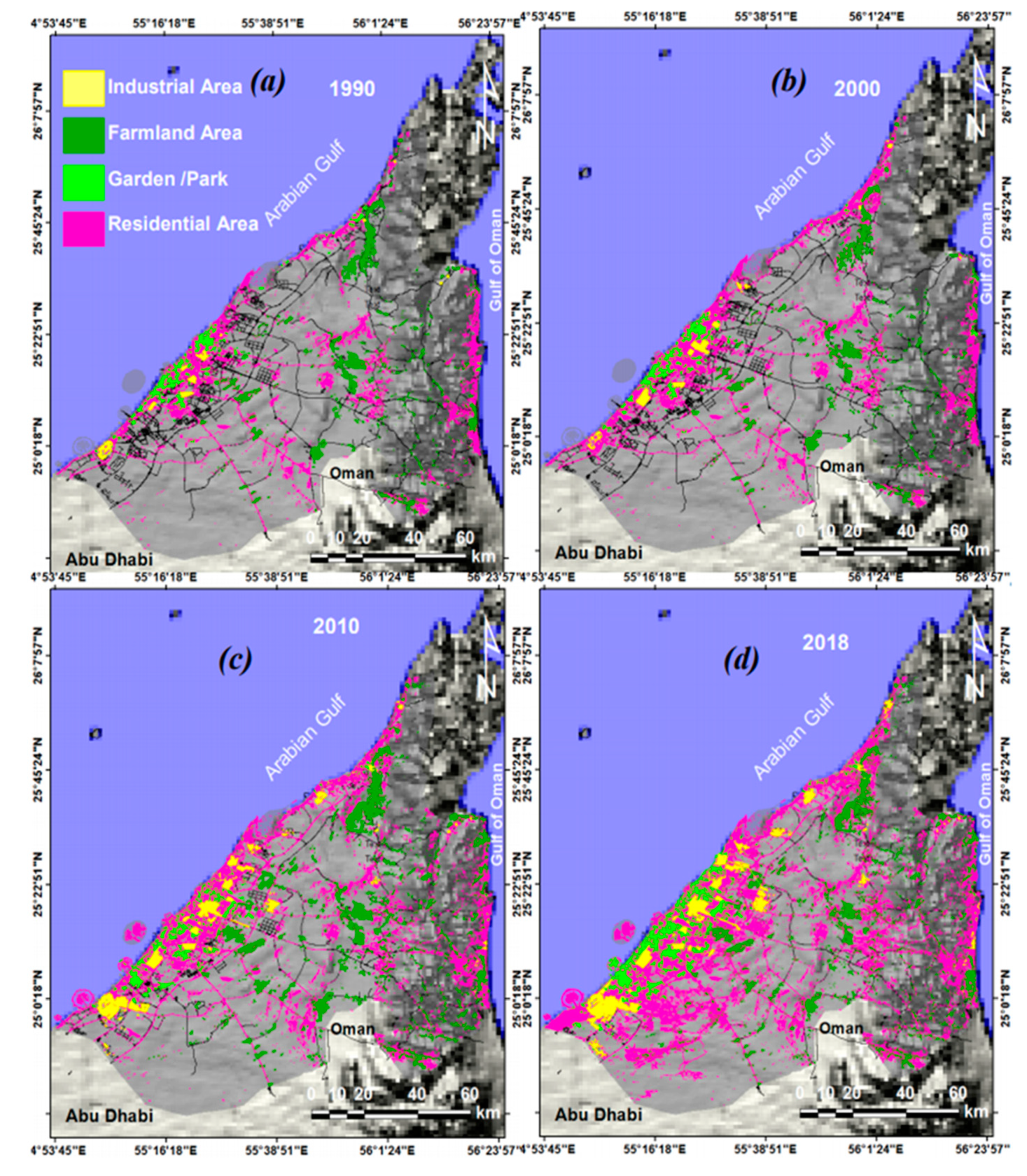
The LULC maps show that built-up areas such as residential and industrial and vegetated areas such as garden/parks are concentrated on the eastern and western coastal areas (coastal aquifers) of the NUAE, while the farmlands and agricultural activities are distributed in sand dune corridors (sand dune aquifer), alluvial plains (alluvial aquifer), and mountainous wadis courses (Ophiolite aquifer).
The built-up and vegetated areas extend like two strips in shapes on the coastal areas. The first strip extends like a triangle in shape, with its head in the city of Ras Al Khaimah and base in the city of Dubai near the Dubai-Abu Dhabi border. The second strip extends like a narrow vertical strip along the eastern coastal area (aquifer) from Dibba in the north to Khor Fakkan in the south of about 60 km in length and about 2 km in width (Figure 6). However, some portion of built-up types and small roads cannot be discriminated against and were misclassified due to the pixel size, moderate spatial resolution, and intensive vegetation cover in a built-up area [47]. The calculated built-up area covered 869.76 km2 (7.40%), while the vegetation area was 254.1 km2 (2.15%) (Figure 6 and Table 4).
From 1990 to 2018, two expansions were clearly observed in the onshore and offshore areas. In the offshore area, the Palm Jumeirah, the Palm Jebel Ali, and the Continental islands were constructed in Dubai covering an area of about 195 km2. In the onshore area, three expansions in the built-up area were observed: the first one in the north-west to the south-east direction, while the second in the west and the east directions (Figure 6 and Figure 7).
3.4. Monitoring LULC Changes
The overall changes in built-up and vegetation areas over the year from 1990 to 2018 and population density measures the number of persons per square kilometres is shown in Figure 7 and details of the changes in LULC classes over 28 years are summarised in Table 5. From 1990 to 2000, the residential area increased from 198.8 km2 (1.69%) to 387.1 (3.30%) with positive change of 188.3 km2 (1.60%), while the industrial area increased from 28.46 km2 (0.24%) to 52.70 km2 (0.44%) with a positive change of 24.24 km2 (0.20%). The gardens/parks slightly increased from 6.93 km2 (0.05%) to 7.19km2 (0.06%) with very slight positive change of 0.26 km2 (0.002%), while farmlands increased from 64.76 km2 (0.55%) to 64.79 km2 (0.55%) without any change.
From 2000 to 2010, the residential area increased from 387.1 km2 (3.30%) to 494.72 km2 (4.21%) with a positive change of 107.62 km2 (0.91%), while the industrial area increased from 52.70 km2 (0.44%) to 168.92 km2 (1.44%) with a positive change of 116.22 km2 (0.99%). From 2010 to 2018, the residential and the industrial areas continue to increase in area by 129.11 km2 (1.10%) and 77.02 km2 (0.65%), respectively. The result also shows that the farmland area decreased from 149.71 km2 (1.27%) to 128.84 km2 (1.09%) with a negative change of −20.87 km2 (0.17%) (Figure 7b). The reason for the farmland decrease (during the period from 2010 to 2018) could be due to the decrease in groundwater level as a response to over-pumping, depletion of groundwater quality, and scarcity of rainfall (Figure 6 and Table 3).
In terms of overall changes, the built-up area, especially in the emirates of Dubai and Sharjah, have grown rapidly in sabkha and sand dune areas towards the southwest and east directions (Figure 7). Spatial analysis of the LULC classes showed that all LULC subclasses (i.e., gardens/parks, farmlands, residential, and industrial) increased in time and space (Figure 6, Figure 7 and Figure 8 and Table 5).
Similarly, the total population of the UAE was observed to increase from 1.8 million in 1990 to 3 million in 2000 and 9.5 million in 2018 with population density distributed in the study area (Figure 7c and Figure 8a).
The reason for the increase built-up and population could be a rapid commercial leap of the Emirate of Dubai, while the sharp increase in the vegetated areas may be due to an increase in the total areas of gardens and golf clubs, which are distributed in the NUAE [47]. From the above results, it is clear that rapid urbanization with a significant expansion in the built-up areas, population growth, gardens, and parks has led to the excessive use of desalinated water and groundwater, and caused considerable changes to groundwater conditions [47]. Additionally, these changes have increased the probability of the occurrence of environmental issues in the next decades, which is consistent with Elmahdy and Mohamed (2018) [47].
The aforementioned results are supported by Elmahdy and Mohamed (2015) (2018) [12,47], who reported that built-up and vegetation areas increased rapidly during the period between 1990 and 2018. They also reported that agricultural cover decreased compared with parks and gardens between 2010 and 2015. This may be due to groundwater level depletion as a response to rainfall scarcity.
3.5. Monitoring Spatiotemporal Variations of Groundwater Level and Quality
Figure 9 shows the interpolated maps constructed from hydrological information collected from 80 groundwater wells distributed across the study area. The maps consist of different colour codes representing the spatial variation of the groundwater level in the study area. The maps show that the groundwater level (depth to groundwater) has sharply dropped down over the 28 years and the depth to groundwater level ranges from 25 m in the coastal areas in the east and the west to 100 m in the alluvial area at the foot of mountainous areas, following the same direction of topographic elevation.
From 1990 to 2018, the groundwater level depleted and some groundwater wells have gone dry in response to over-pumping, especially in the sand dune and alluvial plains where intensive farming is found [49]. As shown in Figure 8, the depth to groundwater level has been depleted in the eastern and western alluvial plains and coastal areas that experienced intensive urbanisation, population growth, and agricultural activity.
Figure 9 shows a hydrologic profile constructed from hydrological information collected from the groundwater wells across the study area. The profile shows two steep slopes in the groundwater level. The first slope is between alluvial plains and coastal areas, and the second, between mountainous and alluvial plains in the east and west.
Along with the coastal areas, the groundwater level declined under sea level with about -25 m (m.s.l) suggesting seawater intrusion. Toward the alluvial plains, a dramatic depletion in the groundwater level was observed. From 1990 to 2000, the groundwater level depleted from 150 to 135 m (m.s.l), and the areas experienced a serious groundwater depletion, increasing from 4.904 km2 to 5.934 km2 with a positive change of about 1030 km2 (8.78 %) (Figure 9a,b and Figure 10). Between 2000 and 2010, the groundwater level dropped slightly from 135 m in 2000 to 128 (m.s.l) m in 2010 and the study area experienced a decline in the groundwater level from 5934 km2 in 2000 to 6698 km2 in 2010 (Figure 9b,c and Figure 10).
From 2010 to 2018, the groundwater level continued to be depleted by about −25 m (a.s.l) and the affected area increased from 6698 km2 in 2010 to 8258 km2 (70.41%) in 2018 (Figure 9c,d and Figure 10). Elmahdy and Mohamed (2014) [48] showed that groundwater quality improves with depth under the water level. As the depth to the water table increases, the groundwater quality increases. Figure 10 shows a regional spatiotemporal variation in NO3 consecration in groundwater wells across the entire areas from 1990 to 2018. It is clearly noticed that there was a dramatic increase in NO3 concentration in groundwater over space and time from the Oman mountains to the coastal areas in the east and the west. The area contaminated by NO3 increased from about 1673 km2 in 1990 to 6178 km2 in 2018 (Figure 11).
Large spots of NO3 concentration were observed in the sand dunes and the alluvial aquifers. The reason for that could be the leaching of salts that accumulated in micro-depressions, alluvial plains, and the shallow aquifer during the last two decades before irrigation activity and LULC development, as well as the intensive use of fertilisation in farmland areas such as Hamranih, Al Dhaid, and Al Awier [50] (Figure 1, Figure 6, Figure 7 and Figure 11). This indicates that nitrate contamination of groundwater in irrigated agricultural land is the main concern in arid and semi-arid regions [12,18]. The sharp increase in NO3 concentration is caused by increasing solutes in groundwater.
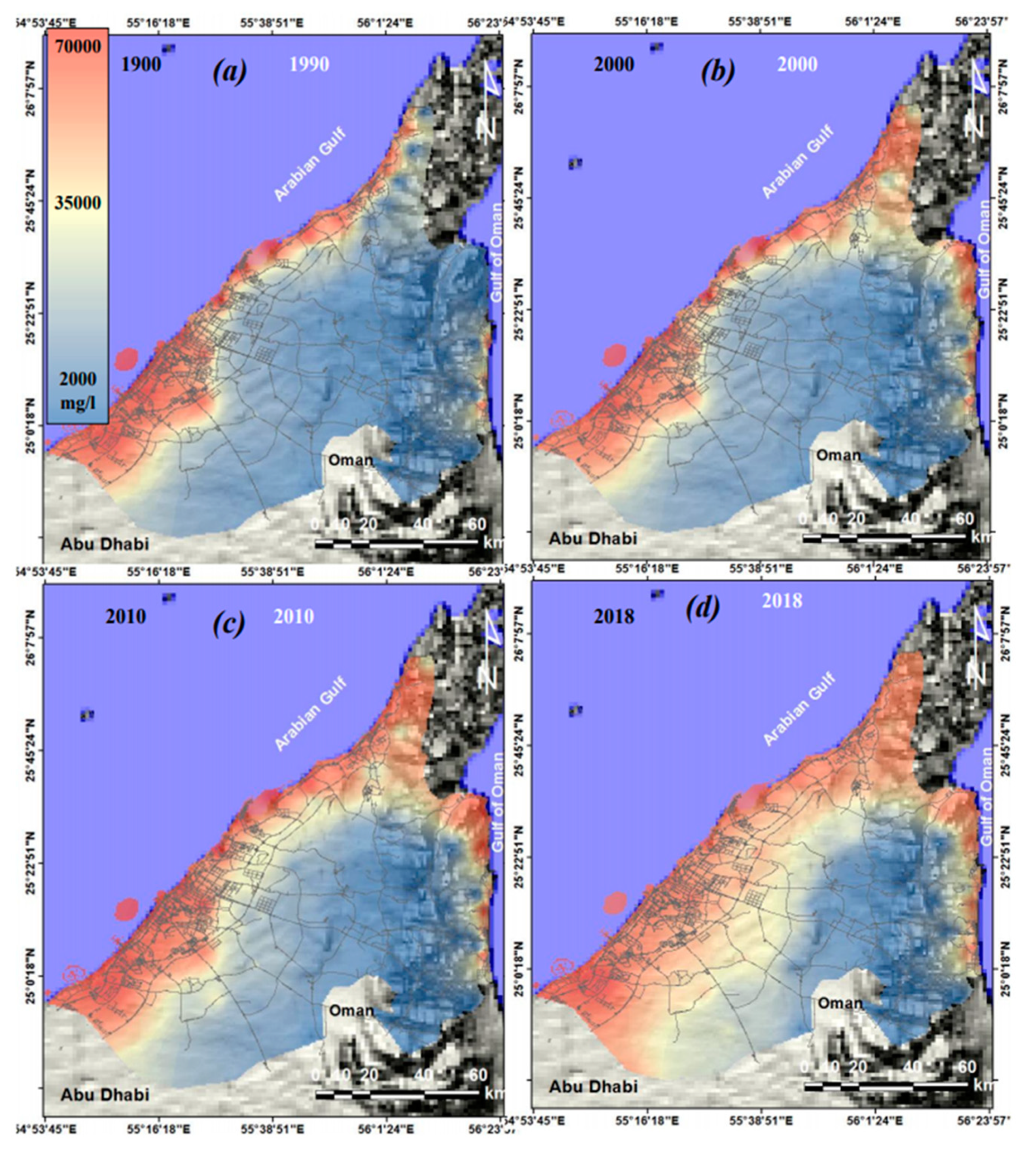
Figure 12 shows a continuous increase in TDS concentration in groundwater across the study area ranging from 2000 in mountainous areas to 70,000 mg/l in the coastal areas, which is double the seawater salinity [50,51,52,53,54]. From 1990 to 2018, the total area influenced by TDS pollutants increased from 2571 km2 (21.91%) in 1990 to 3931 km2 (33.25%) in 2018 (Figure 12).
Towards the coastal areas, a gradual increase of TDS in groundwater was observed. The gradual increase in TDS is attributed to intensive urbanisation, industrial and gardening activities, and the use of fertilizer and retreated water for gardening. The gradual increase in TDS concentration is also attributed to seawater intrusion and the carriage of dissolved and non-dissolved solutes by groundwater flow along the palaeochannels (the wadi courses) during wet seasons [15,18].
Groundwater seeps out of the mountainous areas, dissolves carbonate rocks, mixes dissolved salts with trace elements, and they accumulate along coastal areas.
With distance away from the mountainous areas, TDS concentration in groundwater increases and the groundwater becomes more saline (Figure 12). The dissolution of evaporates, leakage of saline water, and circulation of flow irrigation of the groundwater aquifer are also sources of TDS in groundwater [55,56,57,58,59,60,61]. However, population growth and density have a strong impact on TDS concentration in groundwater in the NUAE.
3.6. Spatial Analysis and Correlation
3.6.1. Impacts of LULC Changes and Population Growth on Groundwater Level
The results show that the connections between urbanisation, population growth, and groundwater level (which is part of water usage) are obvious when comparing the groundwater level depletion rate against the irrigated agricultural and built-up area expansions and population growth (Figure 6, Figure 7, Figure 9 and Figure 13). The population growth trends since 1990 were projected to 2050 to estimate water needs during the next 30 years and the estimated daily water consumption varies from 540 to 570 L per person and total water usage from 100 mcm in 1990 to 3000 mcm in 2018 (Figure 13).
This means that the UAE is consuming groundwater reserves more than 20-fold compared to recharged water, and the UAE may run out of groundwater by 2030 [49]. This relationship was observed between annual population growth and groundwater and water usage (mcm) since 1990 (Figure 13).
The link between population growth, urbanization, and groundwater level is clear when comparing the changes in residential areas and water usage of households (Figure 7 and Figure 14). The rapid changes in the built-up areas and population growth are highly correlated with water usage, including groundwater level (Figure 13 and Figure 14).
A negative relationship between the groundwater level and the irrigated agricultural area is observed (Figure 15). Irrigation of the agricultural sector was found to be the major water consumer, with an average of about 60%, while the water used for industrial and household purposes is about 40% of the total water consumption [19,49,50]. The spatial relationship shows that the areas affected by high NO3 concentration and groundwater depletion are, at the same time, the areas that have the greatest need for water, including the irrigated agricultural areas (Figure 15 and Figure 16).
The impact of vegetation, as part of LULC, on groundwater recharge and groundwater level can be both negative and positive by facilitating the surface water infiltration and transpiration obtained from the rooted soil profile [61,62,63,64,65]. While the irrigated agricultural areas and water demand in the study area increase depletion in the groundwater level and the rate of evapotranspiration (2–3 m/year), the built-up areas decrease water infiltration and the recharge rate (<4%/year) due to their impervious surfaces [12,13,66]. This finding coincides with those of Scanlon et al. (2005) [32], Elmahdy and Mohamed (2016) [12], and Sherif and Singh (1999) [50], who reported that the rainfall scarcity, increase in temperature anomaly and rapid urbanisation, as well as intensive human activities are greatly impacting groundwater levels and quality decline. The sharp depletion of groundwater levels by irrigated agricultural area expansion has led to groundwater depletion, soil and water salinization, and seawater intrusion into the coastal areas, especially in the Emirates of Fujairah and Ras Al Khaimah [27,49,50,51].
3.6.2. Impacts of LULC Changes and Population Growth on Groundwater Quality
A comparison between the maps of LULC changes and groundwater level and quality suggests a strong spatial correlation between LULC changes and groundwater quality. The rapid changes in LULC have led to the degradation of water quality in the entire region. Degradation of groundwater quality and increased TDS concentration is attributed to the leaching and dissolution of salts that are cemented in the soil, intensive use of fertilizers, and irrigation water return flow from agricultural activity to the shallow aquifer [66,67]. The estimated return flow is on average 25% of the total amount of groundwater application [48,49,50]. While the irrigation return flow increases the groundwater recharge, it decreases the groundwater quality and increases NO3 concentration. The intensive use of N fertilisers is well recognised by several studies all over the world that have documented a systematic increase in nitrate concentration in the groundwater due to the long-term intensive application of N fertilisers [54,55,56,57]. The NO3 is the highest concentration of a commonly recognised contaminant in the groundwater [46,57].
The NDVI provides an excellent tool for measuring biomass and characterising landscape dominated by grass (parks/gardens) and agricultural areas [51,52]. From LULC change and NO3 concentration maps (Figure 5, Figure 6, Figure 14, Figure 15 and Figure 16a), it is obvious that the highest value of NO3 almost correlated well with NDVI during 1990 and 2018 (r2 = 0.84) (Figure 16). This finding is consistent with Scanlon et al. (2005), [32] who stated that groundwater and soil quality decrease with increased agricultural and irrigation efficiency, and Chu et al. (2013) [60] who identified the relationship between LULC changes and the water quality.
Figure 17 shows a strong spatial association between septic tanks, sewage treatment plants, landfills, and TDS concentration in the groundwater. The use of unsystematic drainage and septic tanks in the industrial and agricultural areas (e.g., labour camps) is also a significant factor increasing the TDS concentration in the groundwater [18,52].
The wastewater increased from 1.3 Mn3 in 1990 to 4.7 Mn3 in 2018 as a result of increasing population and wastewater discharge from septic tanks and landfills [54]. High TDS concentration in the groundwater appears to be due to sulphates, bicarbonate, carbonate, chloride, sodium, and nitrate, which may originate from natural sources (e.g., carbonate rocks), urban runoff, and agricultural and industrial wastewater [1,18,27,55]. The highest TDS concentration in the groundwater is notably limited to the coastal areas. In the coastal areas, there are rapid urbanisation, septic tanks, sewage treatment plants, and landfills leaking effluent to the shallow aquifer and contaminating the groundwater [46]. The high TDS and Cl- concentration in the groundwater are also positively associated with intensive urbanisation. This phenomenon can be explained by the fact that groundwater level depletion due to overpumping is mainly responsible for groundwater level depletion, and thus seawater intrusion as indicated by the Na/Cl ratio map [49,50,61] (Figure 16d). The low value (<1) for the Na/Cl ratio in the groundwater indicates seawater intrusion and regional brine and sabkha impacts [11,19,49,54,61,62].
The presence of Na+ indicates the dilution influence of water leaking from the sewage pipeline and septic tanks towards groundwater aquifer [62,63,64,65,66,67]. From the point of view of this study, further LULC and climate changes (e.g., rainfall scarcity, increase in air temperature, transpiration, and soil erosion) are expected to influence groundwater levels and quality. Therefore, it is recommended that more efforts are made to control the sources of wastewater discharges (such as septic tanks, landfill and sewage treatment plants as well as cement factories) into the shallow aquifer. Furthermore, unnecessary farms and unsystematic labour camps in residential and agricultural areas should be reconsidered.
4. Conclusion and Recommendation
An integration free of charge monitoring approach based on combining remote sensing data and hydrological information is proposed. This approach was applied to the NUAE to investigate the impact of the LULC changes on groundwater level and quality. The proposed approach and Landsat images with a spatial resolution of 30 m showed a powerful ability for mapping LULC over a regional scale with an overall accuracy of 90.15%–95.14%. The result of confusion metrics, including precision, recall, and F1, indicated that the SVM classifier performs better than SAM classifier.
Almost all types of building and vegetated areas were observed to increase for the periods 1990–2000 and 2000–2010, whereas the period 2010–2018 was characterised by a slight reduction in agricultural area. The results provide strong evidence of the rapid and significant LULC change and population growth in the UAE during the period between 1990 and 2018. The increase in built-up and vegetated areas was accompanied by an increase in population and water consumption and a decrease in desert and coastal areas. These changes may have a considerable impact on the overall water resources and ecosystem implementation. Our results indicate that the study area is experiencing a sharp depletion in groundwater levels in the residential and agricultural areas. Thus, its increasingly susceptible to seawater intrusion and groundwater contamination. The rate of groundwater level depletion and diminished quality has increased continually since the 1990s and is expected to increase year after year. Agricultural and human activities were shown to have a strong correlation with the NO3 concentration (r = 0.91) in the groundwater, while the groundwater level was negatively correlated with NO3.
High TDS concentration is caused by seawater intrusion. Seawater intrusion is caused by overpumping, and overpumping may be caused by an increase in population/farmland increase to fulfill obvious needs. The UAE including the study area is characterised by a scarcity of rainfall and a high rate of evapotranspiration (2–3 m/year), which is very vulnerable to drought and earth subsidence [68,69]. Thus, there is a need for legislation to manage the use of water, and the rapid change in LULC should be controlled. A continued rapid change in LULC represents a serious threat to the hydrological resources of the UAE. The results of the proposed approach provide various information for land-use planners and water resources management. The use of LULC and hydrological maps could elicit a new spatial relationship between rapid LULC changes and land subsidence. Further investigation of the impact of groundwater level depletion (influenced by rapid LULC change) on seawater intrusion and land subsidence is suggested. This investigation permits a better understanding of the impact of the spatiotemporal variations in groundwater level and quality on the environmental and geotechnical setting. Future work should incorporate Sentinel-1 to monitor land subsidence (vertical movement) over the NUAE and support the correlation of results with the rapid changes in LULC and groundwater level.
Author Contributions
Project administration, M.M.; Supervision, T.A.; Writing—original draft, S.E. All authors have read and agreed to the published version of the manuscript.
Acknowledgments
The authors would like to thank the American University of Sharjah, UAE for supporting this research. The research has received funding under financial grant SCRI 18 Grant EN0-284.
Conflicts of Interest
The authors declare no conflict of interest.
References
- Parkinson, J.A. Irrigation in the Near East Region in Figures; Water Report; Food and Agriculture Organization: Rome, Italy, 1997; Volume 9. [Google Scholar]
- Gosling, S.N.; Arnell, N.W. A global assessment of the impact of climate change on water scarcity. Clim. Chang. 2016, 134, 371–385. [Google Scholar] [CrossRef] [Green Version]
- Weber, H.; Sciubba, J.D. The Effect of Population Growth on the Environment: Evidence from European Regions. Eur. J. Popul. 2018, 35, 379–402. [Google Scholar] [CrossRef] [PubMed]
- Patra, S.; Sahoo, S.; Mishra, P.; Mahapatra, S.C. Impacts of urbanization on land use/cover changes and its probable implications on local climate and groundwater level. J. Urban Manag. 2018, 7, 70–84. [Google Scholar] [CrossRef]
- Giri, S.; Singh, A.K. Human health risk assessment via drinking water pathway due to metal contamination in the groundwater of Subarnarekha River Basin, India. Environ. Monit. Assess. 2015, 187, 63. [Google Scholar] [CrossRef] [PubMed]
- Immerzeel, W. Historical trends and future predictions of climate variability in the Brahmaputra basin. Int. J. Clim. 2008, 28, 243–254. [Google Scholar] [CrossRef]
- Kløve, B.; Ala-Aho, P.; Bertrand, G.; Gurdak, J.J.; Kupfersberger, H.; Kværner, J.; Uvo, C.B. Climate change impacts on groundwater and dependent ecosystems. J. Hydrol. 2014, 518, 250–266. [Google Scholar] [CrossRef]
- Mishra, N.; Kumar, S. Impact of Land Use Change on Groundwater Recharge in Haridwar District. In Proceedings of the 20th International Conference on Hydraulics, Water Resources and River Engineering, IIT Roorkee, India, 17–19 December 2015. [Google Scholar]
- Lindquist, L.W.; Palmquist, K.A.; Jordan, S.E.; Lauenroth, W.K. Impacts of climate change on groundwater recharge in Wyoming big sagebrush ecosystems are contingent on elevation. West. N. Am. Nat. 2019, 79, 37–48. [Google Scholar] [CrossRef]
- Elmahdy, S.I.; Mohamed, M.M. Influence of geological structures on groundwater accumulation and groundwater salinity in Musandam Peninsula, UAE and Oman. Geocarto Int. 2013, 28, 453–472. [Google Scholar] [CrossRef]
- Ministry of Environment and Water (MEW). UAE State of Environment Report; Ministry of Environment and Water (MEW): Abu Dhabi, United Arab Emirates, 2015.
- Elmahdy, S.I.; Mohamed, M.M. Land use/land cover change impact on groundwater quantity and quality: A case study of Ajman Emirate, the United Arab Emirates, using remote sensing and GIS. Arab. J. Geosci. 2016, 9, 722. [Google Scholar] [CrossRef]
- Samy, I.E.; Mohamed, M.M. Natural hazards susceptibility mapping in the Kuala Lumpur, Malaysia: An assessment using remote sensing and geographic information system (GIS). Nat. Hazard. Risk 2012, 2012, 1–21. [Google Scholar]
- Mohamed, M.M.; Elmahdy, S.I. Natural and anthropogenic factors affecting groundwater quality in the eastern region of the United Arab Emirates. Arab. J. Geosci. 2015, 8, 7409–7423. [Google Scholar] [CrossRef]
- Sultan, M.; Sturchio, N.; Al Sefry, S.; Milewski, A.; Becker, R.; Nasr, I.; Sagintayev, Z. Geochemical, isotopic, and remote sensing constraints on the origin and evolution of the Rub Al Khali aquifer system, Arabian Peninsula. J. Hydrol. 2008, 356, 70–83. [Google Scholar] [CrossRef]
- Elmahdy, S.I.; Mohamed, M.M. Groundwater of Abu Dhabi Emirate: A regional assessment by means of remote sensing and geographic information system. Arab. J. Geosci. 2015, 8, 11279–11292. [Google Scholar] [CrossRef]
- Nas, B.; Berktay, A. Groundwater quality mapping in urban groundwater using GIS. Environ. Monit. Assess. 2008, 160, 215–227. [Google Scholar] [CrossRef] [PubMed]
- Elmahdy, S.I.; Mohamed, M.M. Remote sensing and geophysical survey applications for delineating near-surface palaeochannels and shallow aquifer in the United Arab Emirates. Geocarto Int. 2015, 30, 723–736. [Google Scholar] [CrossRef]
- JICA (Japanese International Cooperation Agency). The Master Plan Study on the Groundwater Resources Development for Agriculture in the Vicinity of Al Dhaid in the UAE, Final Report; JICA International Cooperation Agency: Sharjah, UAE, 1996.
- Bellot, J.; Bonet, A.; Sanchez, J.R.; Chirino, E. Likely effects of land use changes on the runoff and aquifer recharge in a semiarid landscape using a hydrological model. Landsc. Urban Plan. 2001, 55, 41–53. [Google Scholar] [CrossRef]
- Elmahdy, S.I.; Mohamed, M.M. Factors controlling the changes and spatial variability of Junipers phoenicea in Jabal Al Akhdar, Libya, using remote sensing and GIS. Arab. J. Geosci. 2016, 9, 478. [Google Scholar] [CrossRef]
- Nóbrega, R.L.B.; Guzha, A.C.; Lamparter, G.; Amorim, R.S.S.; Couto, E.G.; Hughes, H.J.; Jungkunst, H.F.; Gerold, G. Impacts of land-use and land-cover change on stream hydrochemistry in the Cerrado and Amazon biomes. Sci. Total Environ. 2018, 635, 259–274. [Google Scholar] [CrossRef]
- Mohamed, M.M.; Elmahdy, S. Land Use/Land Cover Changes Monitoring and Analysis of Dubai Emirate, UAE Using Multi-Temporal Remote Sensing Data. EPiC Ser. Eng. 2018, 3, 1435–1443. [Google Scholar]
- Elmahdy, S.I.; Mohamed, M.M. Automatic detection of near surface geological and hydrological features and investigating their influence on groundwater accumulation and salinity in southwest Egypt using remote sensing and GIS. Geocarto Int. 2014, 30, 132–144. [Google Scholar] [CrossRef]
- Dias, L.C.P.; Macedo, M.N.; Costa, M.H.; Coe, M.T.; Neill, C. Effects of land cover change on evapotranspiration and streamflow of small catchments in the Upper Xingu River Basin, Central Brazil. J. Hydrol. Reg. Stud. 2015, 4, 108–122. [Google Scholar] [CrossRef] [Green Version]
- Haddeland, I.; Heinke, J.; Biemans, H.; Eisner, S.; Flörke, M.; Hanasaki, N.; Stacke, T. Global water resources affected by human interventions and climate change. Proc. Natl. Acad. Sci. USA 2014, 111, 3251–3256. [Google Scholar] [CrossRef] [PubMed] [Green Version]
- Sherif, M.; Almulla, M.; Shetty, A.; Chowdhury, R.K. Analysis of rainfall, PMP and drought in the United Arab Emirates. Int. J. Clim. 2013, 34, 1318–1328. [Google Scholar] [CrossRef]
- Mohamed, M.M.; Elmahdy, S.I. Remote sensing and information value (IV) model for regional mapping of fluvial channels and topographic wetness in the Saudi Arabia. GIScience Remote Sens. 2016, 53, 520–541. [Google Scholar] [CrossRef]
- Zampella, R.A.; Procopio, N.A.; Lathrop, R.G.; Dow, C.L. Relationship of Land-use/Land-cover Patterns and Surface-water Quality in the Mullica River Basin. J. Am. Water Resour. Assoc. 2007, 43, 594–604. [Google Scholar] [CrossRef]
- Pan, Y.; Gong, H.; ZHou, D.; Li, X.; Nakagoshi, N. Impact of land use change on groundwater recharge in Guishui River Basin, China. Chin. Geogr. Sci. 2011, 21, 734–743. [Google Scholar] [CrossRef]
- Kruse, F.A.; Lefkoff, A.B.; Boardman, J.W.; Heidebrecht, K.B.; Shapiro, A.T.; Barloon, P.J.; Goetz, A.F.H. The spectral image processing system (SIPS)—interactive visualization and analysis of imaging spectrometer data. In Proceedings of the AIP Conference, Pasadena, CA, USA, 1 August 1993; American Institute of Physics: Pasadena, CA, USA, 1993; Volume 283, pp. 192–201. [Google Scholar]
- Ha, N.T.; Manley-Harris, M.; Pham, T.D.; Hawes, I. A Comparative Assessment of Ensemble-Based Machine Learning and Maximum Likelihood Methods for Mapping Seagrass Using Sentinel-2 Imagery in Tauranga Harbor, New Zealand. Remote Sens. 2020, 12, 355. [Google Scholar] [CrossRef] [Green Version]
- Scanlon, B.R.; Reedy, R.C.; Stonestrom, D.A.; Prudic, D.E.; Dennehy, K.F. Impact of land use and land cover change on groundwater recharge and quality in the southwestern US. Glob. Chang. Boil. 2005, 11, 1577–1593. [Google Scholar] [CrossRef]
- Le Maitre, D.C.; Scott, D.F.; Colvin, C. A review of information on interactions between vegetation and groundwater. Water S. Afr. 1999, 25, 137–152. [Google Scholar]
- Minnig, M.; Moeck, C.; Radny, D.; Schirmer, M. Impact of urbanization on groundwater recharge rates in Dübendorf, Switzerland. J. Hydrol. 2018, 563, 1135–1146. [Google Scholar] [CrossRef] [Green Version]
- Mittal, R.; Mittal, C.G. Impact of population explosion on environment. WeSchool Knowl. Build. Nat. J. 2013, 1, 1–5. [Google Scholar]
- Foody, G.M. Status of land cover classification accuracy assessment. Remote Sens. Environ. 2002, 80, 185–201. [Google Scholar] [CrossRef]
- Mantero, P.; Moser, G.; Serpico, S.B. Partially supervised classification of remote sensing images through SVM-based probability density estimation. IEEE Trans. Geosci. Remote Sens. 2005, 43, 559–570. [Google Scholar] [CrossRef]
- Support vector machines in remote sensing: A review. ISPRS J. Photogramm. Remote. Sens. 2011, 66, 247–259. [CrossRef]
- Xie, L.; Li, G.; Xiao, M.; Peng, L.; Chen, Q. Hyperspectral image classification using discrete space model and support vector machines. IEEE Geosci. Remote Sens. Lett. 2017, 14, 374–378. [Google Scholar] [CrossRef]
- Lu, D.; Weng, Q.; Moran, E.; Li, G.; Hetrick, S. Remote Sensing Image Classification; CRC Press, Taylor and Francis: Boca Raton, FL, USA, 2011; pp. 219–240. [Google Scholar]
- Van Niel, T.G.; McVicar, T.R.; Datt, B. On the relationship between training sample size and data dimensionality: Monte Carlo analysis of broadband multi-temporal classification. Remote Sens. Environ. 2005, 98, 468–480. [Google Scholar] [CrossRef]
- Congalton, R.G. Putting the map back in map accuracy assessment. Remote Sens. GIS Accuracy Assess. 2004, 5, 1–11. [Google Scholar]
- Jensen, J.R.; Cowen, D.; Huang, X.; Graves, D.; He, K.; Mackey, H.E. Remote sensing image browse and archival systems. Geocarto Int. 1996, 11, 33–42. [Google Scholar] [CrossRef]
- Setianto, A.; Triandini, T. Comparison of kriging and inverse distance weighted (IDW) interpolation methods in lineament extraction and analysis. J. Appl. Geol. 2013, 5, 21–29. [Google Scholar] [CrossRef]
- Elmahdy, S.I.; Mohamed, M.M. Groundwater potential modelling using remote sensing and GIS: A case study of the Al Dhaid area, United Arab Emirates. Geocarto Int. 2013, 29, 433–450. [Google Scholar] [CrossRef]
- Elmahdy, S.I.; Mohamed, M.M. Monitoring and analysing the Emirate of Dubai’s land use/land cover changes: An integrated, low-cost remote sensing approach. Int. J. Digit. Earth 2017, 11, 1132–1150. [Google Scholar] [CrossRef]
- Elmahdy, S.I.; Mohamed, M.M. Relationship between geological structures and groundwater flow and groundwater salinity in Al Jaaw Plain, United Arab Emirates; mapping and analysis by means of remote sensing and GIS. Arab. J. Geosci. 2013, 7, 1249–1259. [Google Scholar] [CrossRef]
- Brook, M.; Dawoud, M.A. Coastal Water Resources Management in the United Arab Emirates; Integrated Coastal Zone Management in the United Arab Emirates: Abu Dhabi, United Arab Emirates (UAE), 2005; pp. 1–12. [Google Scholar]
- Sherif, M.M.; Singh, V.P. Effect of climate change on sea water intrusion in coastal aquifers. Hydrol. Process. 1999, 13, 1277–1287. [Google Scholar] [CrossRef]
- Mahmood, R.; Pielke, R.A., Sr.; Hubbard, K.G.; Niyogi, D.; Bonan, G.; Lawrence, P.; Qian, B. Impacts of land use/land cover change on climate and future research priorities. Bull. Am. Meteorol. Soc. 2010, 91, 37–46. [Google Scholar] [CrossRef]
- Zhou, Y.; Wenninger, J.; Yang, Z.; Yin, L.; Huang, J.; Hou, L.; Wang, X.; Zhang, D.; Uhlenbrook, S. Groundwater-surface water interactions, vegetation dependencies and implications for water resources management in the semi-arid Hailiutu River catchment, China—A synthesis. Hydrol. Earth Syst. Sci. 2013, 17, 2435–2447. [Google Scholar] [CrossRef] [Green Version]
- Ojeda Olivares, E.A.; Sandoval Torres, S.; Belmonte Jiménez, S.I.; Campos Enríquez, J.O.; Zignol, F.; Reygadas, Y.; Tiefenbacher, J.P. Climate Change, Land Use/Land Cover Change, and Population Growth as Drivers of Groundwater Depletion in the Central Valleys, Oaxaca, Mexico. Remote Sens. 2019, 11, 1290. [Google Scholar] [CrossRef] [Green Version]
- Wakode, H.B.; Baier, K.; Jha, R.; Azzam, R. Impact of urbanization on groundwater recharge and urban water balance for the city of Hyderabad, India. Int. Soil Water Conserv. Res. 2018, 6, 51–62. [Google Scholar] [CrossRef]
- Sharp, J.M. The impacts of urbanization on groundwater systems and recharge. Aqua Mundi 2010, 1. [Google Scholar] [CrossRef]
- Mas-Pla, J.; Menció, A. Groundwater nitrate pollution and climate change: Learnings from a water balance-based analysis of several aquifers in a western Mediterranean region (Catalonia). Environ. Sci. Pollut. Res. 2018, 26, 2184–2202. [Google Scholar] [CrossRef] [Green Version]
- Qin, R.; Wu, Y.; Xu, Z.; Xie, D.; Zhang, C. Assessing the impact of natural and anthropogenic activities on groundwater quality in coastal alluvial aquifers of the lower Liaohe River Plain, NE China. Appl. Geochem. 2013, 31, 142–158. [Google Scholar] [CrossRef]
- Appelo, C.A.J.; Postma, D. Geochemistry, Groundwater and Pollution; Balkema: Rotterdam, The Netherlands, 1999; p. 636. [Google Scholar]
- Zhu, B.; Yang, X.; Rioual, P.; Qin, X.; Liu, Z.; Xiong, H.; Yu, J. hydrogeochemistry of three watersheds (the Erlqis, Zhungarer and Yili) in northern Xinjiang, NW China. Appl. Geochem. 2011, 26, 1535–1548. [Google Scholar] [CrossRef]
- Chu, H.J.; Liu, C.Y.; Wang, C.K. Identifying the relationships between water quality and land cover changes in the tseng-wen reservoir watershed of Taiwan. Int. J. Environ. Res. Public Health 2013, 10, 478–489. [Google Scholar] [CrossRef] [PubMed] [Green Version]
- Al-Hogaraty, E.A.; Rizk, Z.S.; Garamoon, H.K. Groundwater pollution of the quaternary aquifer in northern United Arab Emirates. Water Air Soil Pollut. 2008, 190, 323–341. [Google Scholar] [CrossRef]
- McMahon, P.B. Water Movement through Thick Unsaturated Zones Overlying the Central High Plains Aquifer, Southwestern Kansas, 2000–2001; US Department of the Interior, US Geological Survey: Lawrence, KS, USA, 2003; Volume 3.
- Al-Rashed, M.; Sherif, M.M. Water Resources in the GCC Countries: An Overview. Water Resour. Manag. 2000, 14, 59–75. [Google Scholar] [CrossRef]
- Daniëls, E.E. Land Surface Impacts on Precipitation in the Netherlands. Ph.D. Thesis, Wageningen University, Wageningen, The Netherlands, 2016. [Google Scholar]
- Gebru, B.M.; Lee, W.K.; Khamzina, A.; Lee, S.G.; Negash, E. Hydrological Response of Dry Afromontane Forest to Changes in Land Use and Land Cover in Northern Ethiopia. Remote. Sens. 2019, 11, 1905. [Google Scholar] [CrossRef] [Green Version]
- Shahin, S.; Salem, M.A. The Challenges of Water Scarcity and the Future of Food Security in the United Arab Emirates (UAE). Nat. Resour. Conserv. 2015, 3, 1–6. [Google Scholar] [CrossRef] [Green Version]
- Saou, A.; Maza, M.; Seidel, J.L. Hydrogeochemical Processes Associated with Double Salinization of Water in an Algerian Aquifer, Carbonated and Evaporitic. Pol. J. Environ. Stud. 2012, 21, 1013–1024. [Google Scholar]
- Cantone, A.; Riccardi, P.; Baker, H.A.; Pasquali, P.; Closson, D.; Karaki, N.A. Monitoring Small land Subsidence Phenomena in the Al-Ain Region by Satellite SAR Interferometric Stacking. In Proceedings of the Second EAGE International Conference on Engineering Geophysics, Al-Ain, UAE, 24–27 Novmber 2013. [Google Scholar]
- Liosis, N.; Marpu, P.R.; Pavlopoulos, K.; Ouarda, T.B. Ground subsidence monitoring with SAR interferometry techniques in the rural area of Al Wagan, UAE. Remote. Sens. Environ. 2018, 216, 276–288. [Google Scholar] [CrossRef]
Figure 1.
Elevation map generated from a DEM showing the location of the study area and main cities and.
Figure 1.
Elevation map generated from a DEM showing the location of the study area and main cities and.

Figure 2.
Monthly temperature and precipitation (a), number of days of rainfall (b), and daily precipitation (c) over the NUAE.
Figure 2.
Monthly temperature and precipitation (a), number of days of rainfall (b), and daily precipitation (c) over the NUAE.
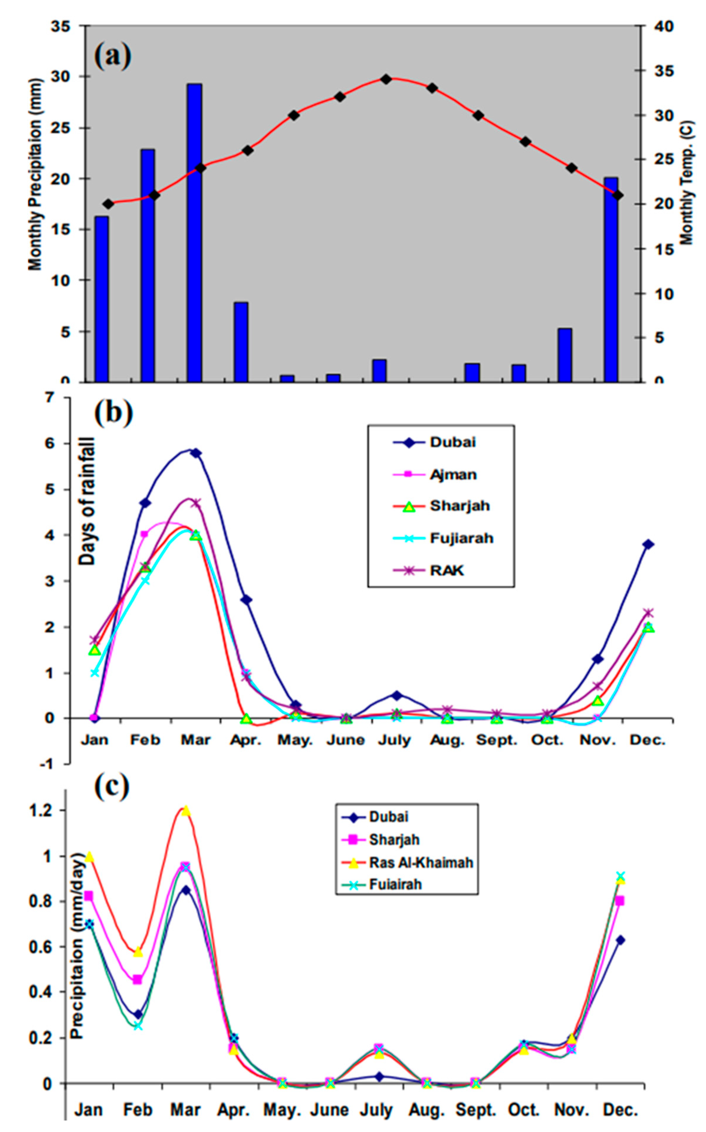
Figure 3.
Maps of the spatial distribution of rainfall (a) and air temperature (b), and geohydrology (c), and wadi courses and palaeochannels generated from a DEM (d) of the study area.
Figure 3.
Maps of the spatial distribution of rainfall (a) and air temperature (b), and geohydrology (c), and wadi courses and palaeochannels generated from a DEM (d) of the study area.
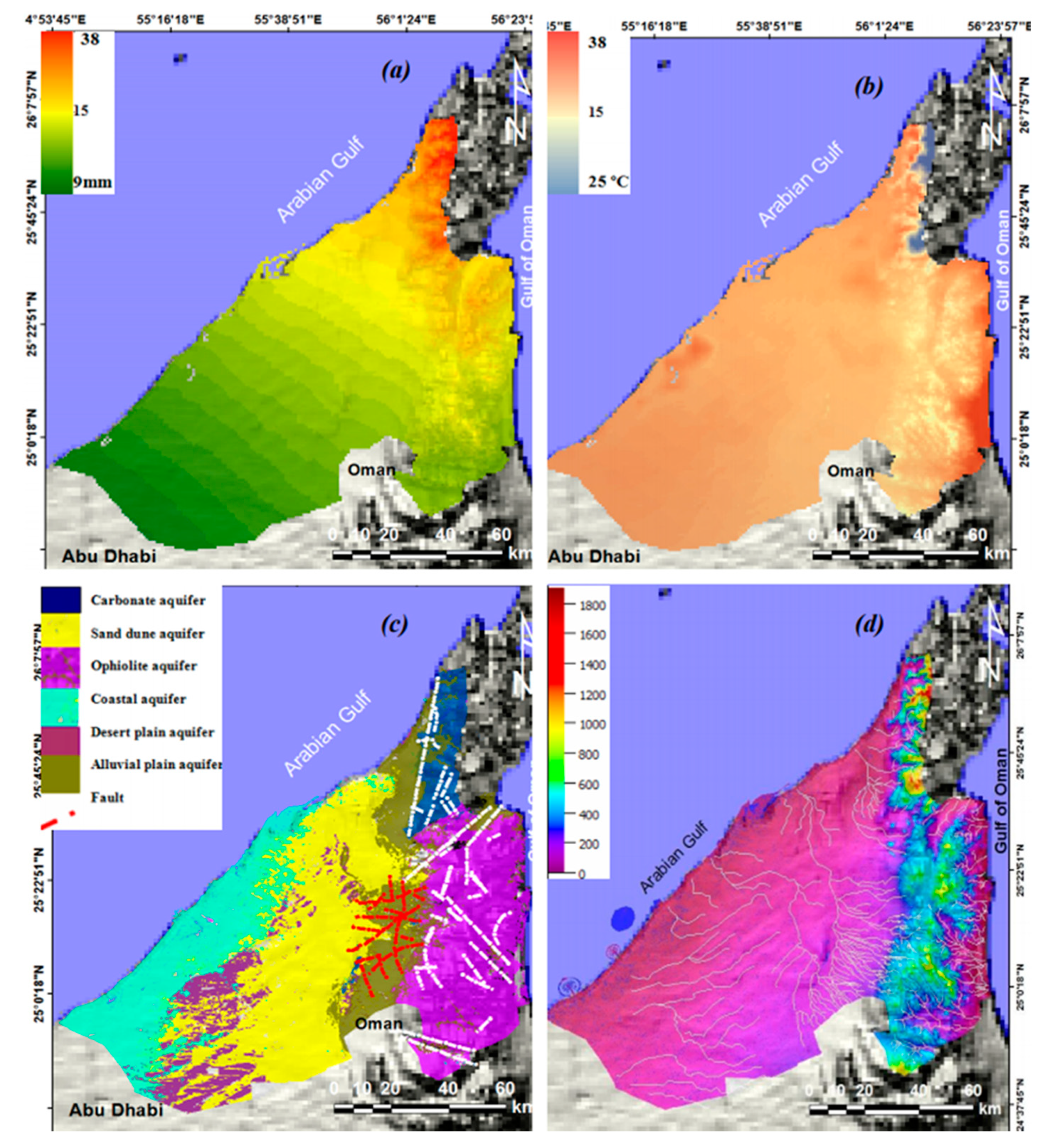
Figure 4.
Flowchart of the methodology applied to the study area.
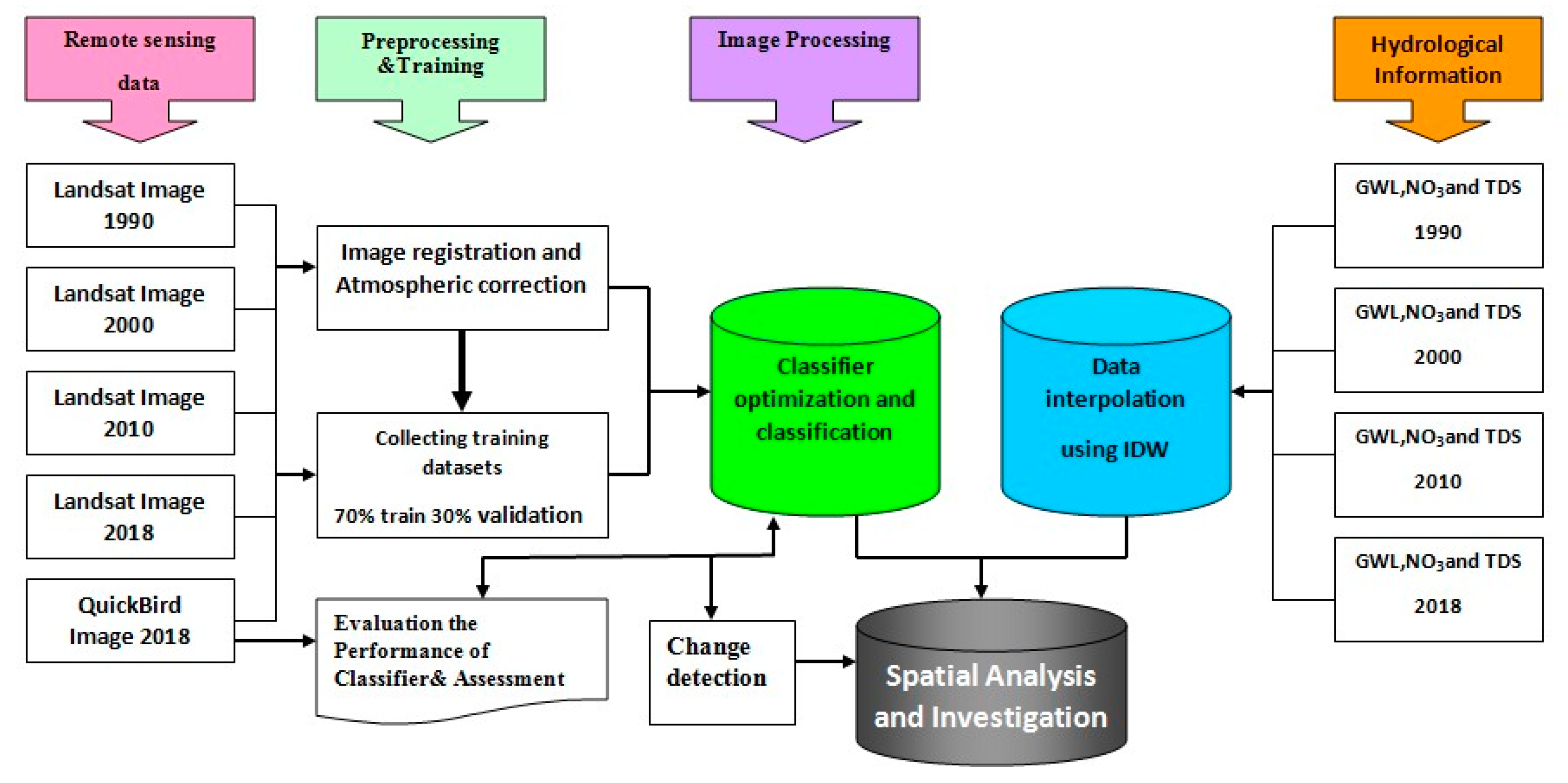
Figure 5.
A comparison of the F1, precision, and recall scores for the Landsat image (15 August 2018) using SVM and SAM classifiers.
Figure 5.
A comparison of the F1, precision, and recall scores for the Landsat image (15 August 2018) using SVM and SAM classifiers.

Figure 6.
Spatiotemporal variation of built-up and vegetation areas of the NUAE during 1990, 2000, 2010, and 2018. Bare land such as sand dune, desert plain, Ophiolite rock was excluded.
Figure 6.
Spatiotemporal variation of built-up and vegetation areas of the NUAE during 1990, 2000, 2010, and 2018. Bare land such as sand dune, desert plain, Ophiolite rock was excluded.

Figure 7.
The overall change in the areas of built-up (a), and vegetation (b) from 1990 to 2018, and (c) population density of the NUAE. The red line separates the garden/ parks and farmlands. The population density measures the numbers of persons per square meter. These maps are draped over a DEM.
Figure 7.
The overall change in the areas of built-up (a), and vegetation (b) from 1990 to 2018, and (c) population density of the NUAE. The red line separates the garden/ parks and farmlands. The population density measures the numbers of persons per square meter. These maps are draped over a DEM.
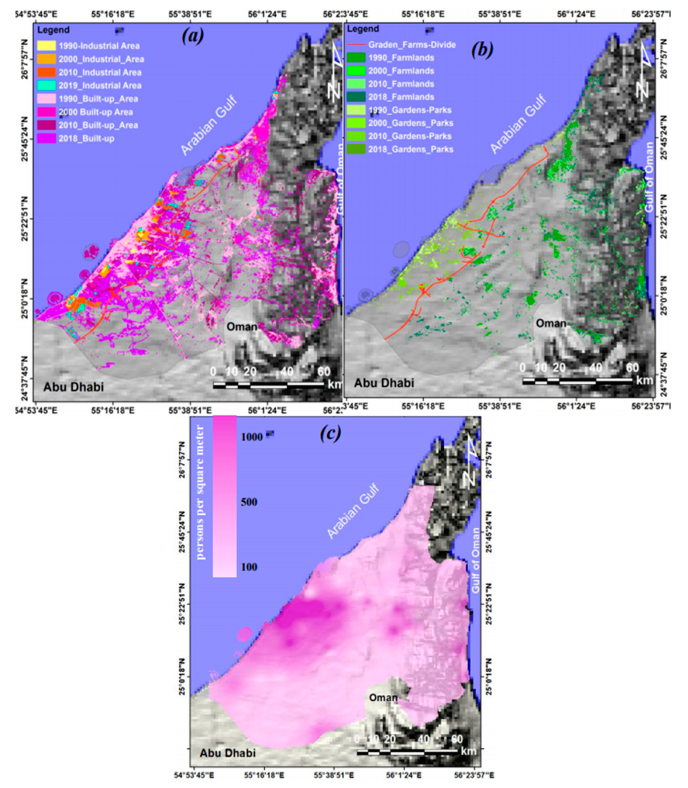
Figure 8.
The graphical representation of the total area in km2 of built-up and vegetated area changes (a), and their differences from 1990 to 2018 (b).
Figure 8.
The graphical representation of the total area in km2 of built-up and vegetated area changes (a), and their differences from 1990 to 2018 (b).


Figure 9.
Regional spatial distribution of the groundwater level depletion (in m) in the NUAE from 1990 to 2018.
Figure 9.
Regional spatial distribution of the groundwater level depletion (in m) in the NUAE from 1990 to 2018.

Figure 10.
E-W hydrological profile constructed from hydrological information collected from selected groundwater wells showing the spatial and temporal variations of groundwater level for the years 1990, 2000, 2010, and 2018.
Figure 10.
E-W hydrological profile constructed from hydrological information collected from selected groundwater wells showing the spatial and temporal variations of groundwater level for the years 1990, 2000, 2010, and 2018.

Figure 11.
Regional spatial and temporal variations of nitrate concentration in groundwater across the study area for the years 1990, 2000, 2010, and 2018.
Figure 11.
Regional spatial and temporal variations of nitrate concentration in groundwater across the study area for the years 1990, 2000, 2010, and 2018.

Figure 12.
Regional spatiotemporal variations of TDS concentration in groundwater wells across the study area for the years 1990, 2000, 2010, and 2018.
Figure 12.
Regional spatiotemporal variations of TDS concentration in groundwater wells across the study area for the years 1990, 2000, 2010, and 2018.

Figure 13.
Relationship between annual population growth and water usage (mcm).

Figure 14.
Relationship between built-up area (km2) and water usage of household (mcm) and groundwater level (m).
Figure 14.
Relationship between built-up area (km2) and water usage of household (mcm) and groundwater level (m).

Figure 15.
Spatiotemporal variations of water usage (mcm), and groundwater level vs the coverage of the irrigated agricultural area.
Figure 15.
Spatiotemporal variations of water usage (mcm), and groundwater level vs the coverage of the irrigated agricultural area.

Figure 16.
Relationship between NO3 concentration in groundwater and calculated NDVI (r2 = 0.84) based on hydrological information collected from groundwater wells and NDVI calculated from satellite images.
Figure 16.
Relationship between NO3 concentration in groundwater and calculated NDVI (r2 = 0.84) based on hydrological information collected from groundwater wells and NDVI calculated from satellite images.
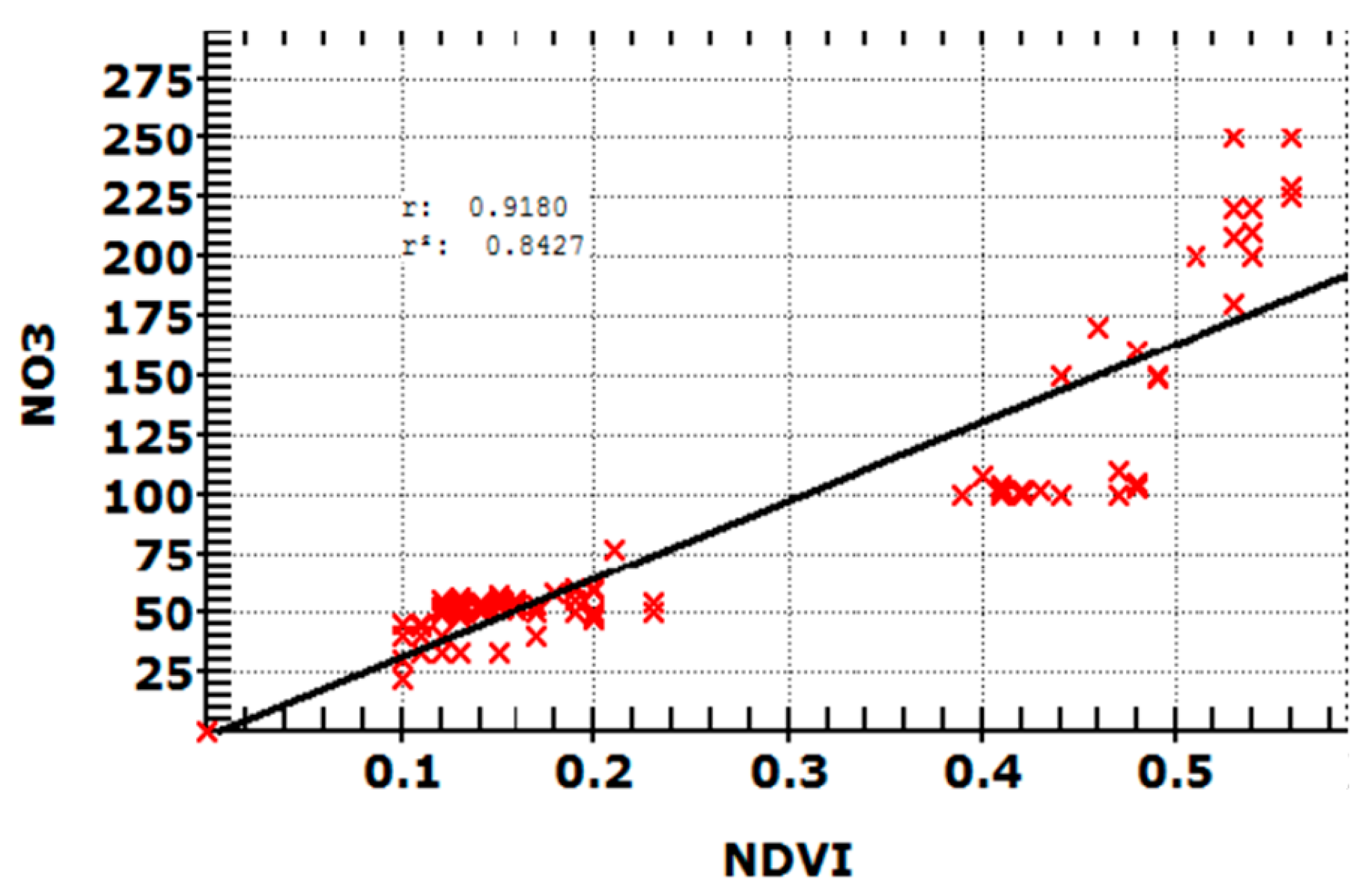
Figure 17.
Built-up and vegetation areas draped over the maps of groundwater level (a), locations of septic tanks, sewage treatment plants, landfill, and farmland are draped over the maps of NO3 and TDS for the year 2018 (b,c), and map of the Na/Cl ratio showing the area affected by water intrusion in 2018 (d).


Table 1.
Characteristics of Landsat and QuickBird images used in the study area.
| Bands | Resolution (m) | Wavelength (mm) | |
|---|---|---|---|
| Thematic Mapper (TM)and Enhanced Thematic Mapper Plus (ETM+) (23 August 1990) (23 August 2000) | Band 1 | 30 | 0.45–0.52 |
| Band 2 | 30 | 0.52–0.60 | |
| Band 3 | 30 | 0.63–0.69 | |
| Band 4 | 30 | 0.77–0.90 | |
| Band 5 | 30 | 1.55–1.75 | |
| Band 6 | 60*(30) | 10.40–12.50 | |
| Band 7 | 30 | 2.09–2.35 | |
| Band 8 | 15 | 0.52–0.90 | |
| Landsat 8 Operational Land Imager (OLI)and thermal infrared sensor (TIRS) (15 August 2018) | Band 1 Coastal aerosol | 30 | 0.43–0.45 |
| Band 2 Blue | 30 | 0.45–0.51 | |
| Band 3 Red | 30 | 0.53–0.59 | |
| Band 4 Red | 30 | 0.64–0.67 | |
| Band 5 Near Infrared (NIR) | 30 | 0.85–0.88 | |
| Band 6 SWIR 1 | 30 | 1.57–1.65 | |
| Band 7 SWIR 2 | 30 | 2.11–2.29 | |
| Band 8 Panchromatic | 0.50–0.68 | ||
| Band 9 Cirrus | 30 | 1.36–1.38 | |
| Band 10 Thermal Infrared (TIRS) 1 | 100*(30) | 10.60–11.19 | |
| Band 11 Thermal Infrared (TIRS) 2 | 100*(30) | 11.50–12.51 | |
| QuickBird (27 August 2018) | B1 Blue | 450–520 | |
| B2 Green | 520–600 | ||
| B3 Red | 630–690 | ||
| Near IR | 760–900 | ||
| Pan | 450–900 |
Table 2.
The SVM algorithm option tested to classify LULC.
| γ | P | Threshold | C |
|---|---|---|---|
| 0.1 | 0 | 0.02 | 100 |
| 0.03 | 1 | 0.03 | 100 |
| 0.005 | 2 | 0.05 | 120 |
| 0.007 | 2 | 0.04 | 110 |
Table 3.
Overall accuracy (%) of the LULC maps for the years 1990, 2000, 2010 and 2018.
| 1990 | 2000 | 2010 | 2018 | |
|---|---|---|---|---|
| Overall Accuracy (%) | 90.15 | 91.35 | 93.01 | 95.14 |
| Kappa Coefficient | 0.811 | 0.841 | 0.88 | 0.918 |
Table 4.
LULC classes estimation (in km2 and percentage) for the years 1990,2000,2010, and 2018 1.
| Class | Subclass | 1990 | 2000 | 2010 | 2018 | ||||
|---|---|---|---|---|---|---|---|---|---|
| (km2) | (%) | (km2) | (%) | (km2) | (%) | (km2) | (%) | ||
| Build-up | Residential | 198.8 | 1.69 | 387.1 | 3.30 | 494.72 | 4.21 | 623.83 | 5.31 |
| Industrial | 28.46 | 0.24 | 52.70 | 0.44 | 168.92 | 1.44 | 245.94 | 2.09 | |
| Vegetation | Park/garden | 6.93 | 0.05 | 7.19 | 0.06 | 67.18 | 0.57 | 125.26 | 1.06 |
| Farmland | 64.76 | 0.55 | 64.79 | 0.55 | 149.71 | 1.27 | 128.84 | 1.09 | |
1 Total Area NUAE 11,727 km2.
Table 5.
Estimates of LULC changes (in km2 and percentage) from 1990 to 2018.
| Class | Subclass | 1990–2000 | 2000–2010 | 2010–2018 | 1990–2018 | ||||
|---|---|---|---|---|---|---|---|---|---|
| (km2) | (%) | (km2) | (%) | (km2) | (%) | (km2) | (%) | ||
| Build-up | Residential | 188.3 | 1.60 | 107.62 | 0.91 | 129.11 | 1.10 | 425.03 | 3.62 |
| Industrial | 24.24 | 0.20 | 116.22 | 0.99 | 77.02 | 0.65 | 217.48 | 1.85 | |
| Vegetation | Park/garden | 0.26 | 0.002 | 59.99 | 0.51 | 58.08 | 0.49 | 118.33 | 1.0 |
© 2020 by the authors. Licensee MDPI, Basel, Switzerland. This article is an open access article distributed under the terms and conditions of the Creative Commons Attribution (CC BY) license (http://creativecommons.org/licenses/by/4.0/).
Share and Cite
MDPI and ACS Style
Elmahdy, S.; Mohamed, M.; Ali, T. Land Use/Land Cover Changes Impact on Groundwater Level and Quality in the Northern Part of the United Arab Emirates. Remote Sens. 2020, 12, 1715. https://doi.org/10.3390/rs12111715
AMA Style
Elmahdy S, Mohamed M, Ali T. Land Use/Land Cover Changes Impact on Groundwater Level and Quality in the Northern Part of the United Arab Emirates. Remote Sensing. 2020; 12(11):1715. https://doi.org/10.3390/rs12111715
Chicago/Turabian StyleElmahdy, Samy, Mohamed Mohamed, and Tarig Ali. 2020. "Land Use/Land Cover Changes Impact on Groundwater Level and Quality in the Northern Part of the United Arab Emirates" Remote Sensing 12, no. 11: 1715. https://doi.org/10.3390/rs12111715
Note that from the first issue of 2016, this journal uses article numbers instead of page numbers. See further details here.