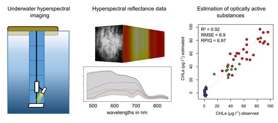
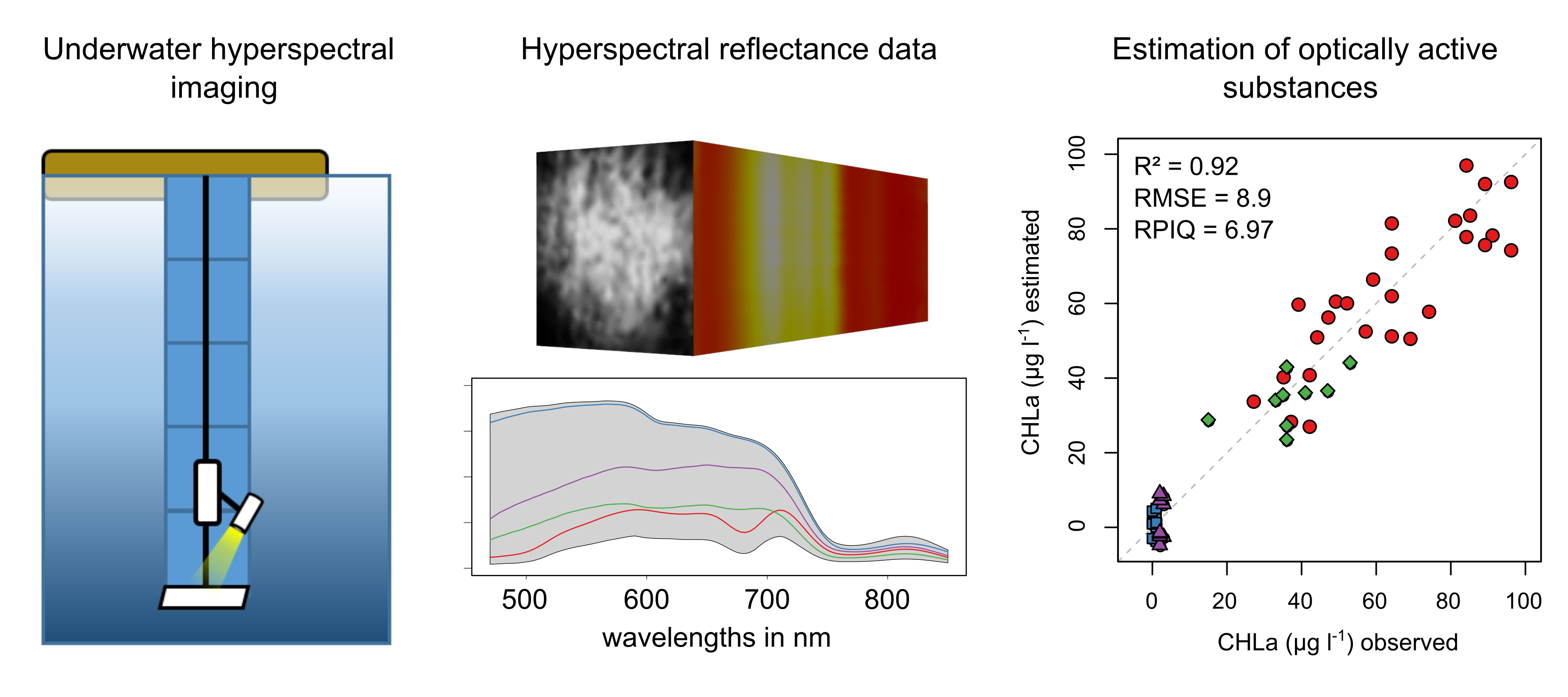
Underwater Use of a Hyperspectral Camera to Estimate Optically Active Substances in the Water Column of Freshwater Lakes

Abstract

Freshwater lakes provide many important ecosystem functions and services to support biodiversity and human well-being. Proximal and remote sensing methods represent an efficient approach to derive water quality indicators such as optically active substances (OAS). Measurements of above-ground remote and in situ proximal sensors, however, are limited to observations of the uppermost water layer. We tested a hyperspectral imaging system, customized for underwater applications, with the aim to assess concentrations of chlorophyll a (CHLa) and colored dissolved organic matter (CDOM) in the water columns of four freshwater lakes with different trophic conditions in Central Germany. We established a measurement protocol that allowed consistent reflectance retrievals at multiple depths within the water column independent of ambient illumination conditions. Imaging information from the camera proved beneficial for an optimized extraction of spectral information since low signal areas in the sensor’s field of view, e.g., due to non-uniform illumination, and other interfering elements, could be removed from the measured reflectance signal for each layer. Predictive hyperspectral models, based on the 470 nm–850 nm reflectance signal, yielded estimates of both water quality parameters (R² = 0.94, RMSE = 8.9 µg L⁻¹ for CHLa; R² = 0.75, RMSE = 0.22 m⁻¹ for CDOM) that were more accurate than commonly applied waveband indices (R² = 0.83, RMSE = 13.2 µg L⁻¹ for CHLa; R² = 0.66, RMSE = 0.25 m⁻¹ for CDOM). Underwater hyperspectral imaging could thus facilitate future water monitoring efforts through the acquisition of consistent spectral reflectance measurements or derived water quality parameters along the water column, which has the potential to improve the link between above-surface proximal and remote sensing observations and in situ point-based water probe measurements for ground truthing or to resolve the vertical distribution of OAS.

1. Introduction

Lake ecosystems provide essential functions and services, including contributions to biodiversity, hydrologic regulation and water supply, and human well-being through their recreational benefits [1,2]. At the same time, they are subject to various threats from climate change, alterations of catchment land use, anthropogenic pollutants, aquatic invasive species, or human harvest including aquaculture [3]. Hence, appropriate monitoring adapted to relevant temporal and spatial scales is necessary for an improved understanding of lake ecosystems and their feedbacks.

Remote sensing in the visible and near-infrared (VNIR) range (400–1000 nm) allows for the spatio-temporal monitoring of various water quality parameters in freshwater lakes [4,5]. The most important indicators of water quality, in general, are phytoplankton, colored dissolved organic matter (CDOM) and total suspended matter (TSM), which represent optically active substances (OAS) [4,6]. Changes in the quantity of the OAS have a direct effect on the spectral signature detected by remote (or proximal) sensors, which, in turn, enables the estimation of OAS contents from measured spectra through physically-based analytical or empirical models [4,7,8]. Nevertheless, in the case of optically complex inland water bodies, the variety of OAS concentrations and their specific inherent optical properties is wide and independent from each other [6,9]. This complexity limits the use of simple band ratio approaches and might affect the accuracy of analytical models due to partly unknown optical properties of contributing OAS [7,10].

Beyond this, the general application of remote sensing methods may be limited, e.g., by cloud cover during overflight. Accurate atmospheric correction is another critical issue for retrieving surface reflectances from remotely sensed data; inaccuracies might affect the OAS retrieval, especially in the case of optically complex inland waters [9,11,12,13,14].

While remote sensing observations can per se provide consistent, spatially-distributed measurements of water quality parameters at large scales, such spectral measurements can be limited by the lake specific penetration depth of light, which might be shallower than the actual constituent layer; otherwise the constituent layer might just form a thin layer within the remotely sensed water layer [15,16,17,18]. Consequently, remotely-sensed measurements cannot resolve the distribution of constituents in the water column, which may impede the correct retrieval of column OAS contents when strong density gradients occur in the remotely-sensed water layer and below.

Water-quality probes, on the other hand, can acquire information from the entire water column, which is relevant, for example, for a series of ecological issues including the detection and analysis of the deep chlorophyll maximum as a hot spot of primary production and nutrient cycling [19]. Besides OAS such as CHLa and CDOM, these sensors can also retrieve additional water parameters including, e.g., temperature, dissolved oxygen, conductivity and pH (e.g., [20,21,22]). Remote sensing and in situ methods can therefore complement each other, for example by allowing ground truthing of satellite-derived biochemical data products or, conversely, the extension of point information across larger spatial scales [23].

In this context, the in situ hyperspectral measurement of water columns, from the uppermost layer observable by remote sensing through deeper layers that are limited to point sensor observations, offers the potential to improve the link between in situ water monitoring networks and Earth observation systems through consistent radiometric measurements along a water profile. Various studies have used hyperspectral point or imaging sensors to provide ground truth data for overflight campaigns and to validate satellite imagery products (e.g., [22,24,25]), but also for the direct derivation of OAS products for water monitoring purposes [21,26,27]. Recently, Keller et al. (2018) [21] deployed a hyperspectral snapshot camera mounted on a boat to collect hyperspectral imagery (450–950 nm) along the Elbe river in Germany with the goal to quantify multiple OAS such as CDOM and CHLa. While they could successfully estimate OAS quantities with surface measurements, it could also be advantageous to transfer this technology into the water column to measure OAS at multiple depths with the same device.

In this study, we evaluated the capabilities of a hyperspectral snapshot camera system to resolve the vertical distribution of CHLa and CDOM in pre-defined segments in the water column. The camera’s spectral imaging quality and capabilities for underwater sensing were first tested in a laboratory experiment against a well-established point spectrometer. Afterward, we conducted a field campaign with multiple water column measurements in four freshwater lakes in Central Germany with the aims to (i) develop an approach to measure water column reflectance without distortions through variations in ambient illumination and (ii) to estimate CHLa and CDOM concentrations through multivariate calibrations with partial least squares regression (PLSR) in comparison to commonly applied CHLa and CDOM indices.

2. Materials and Methods

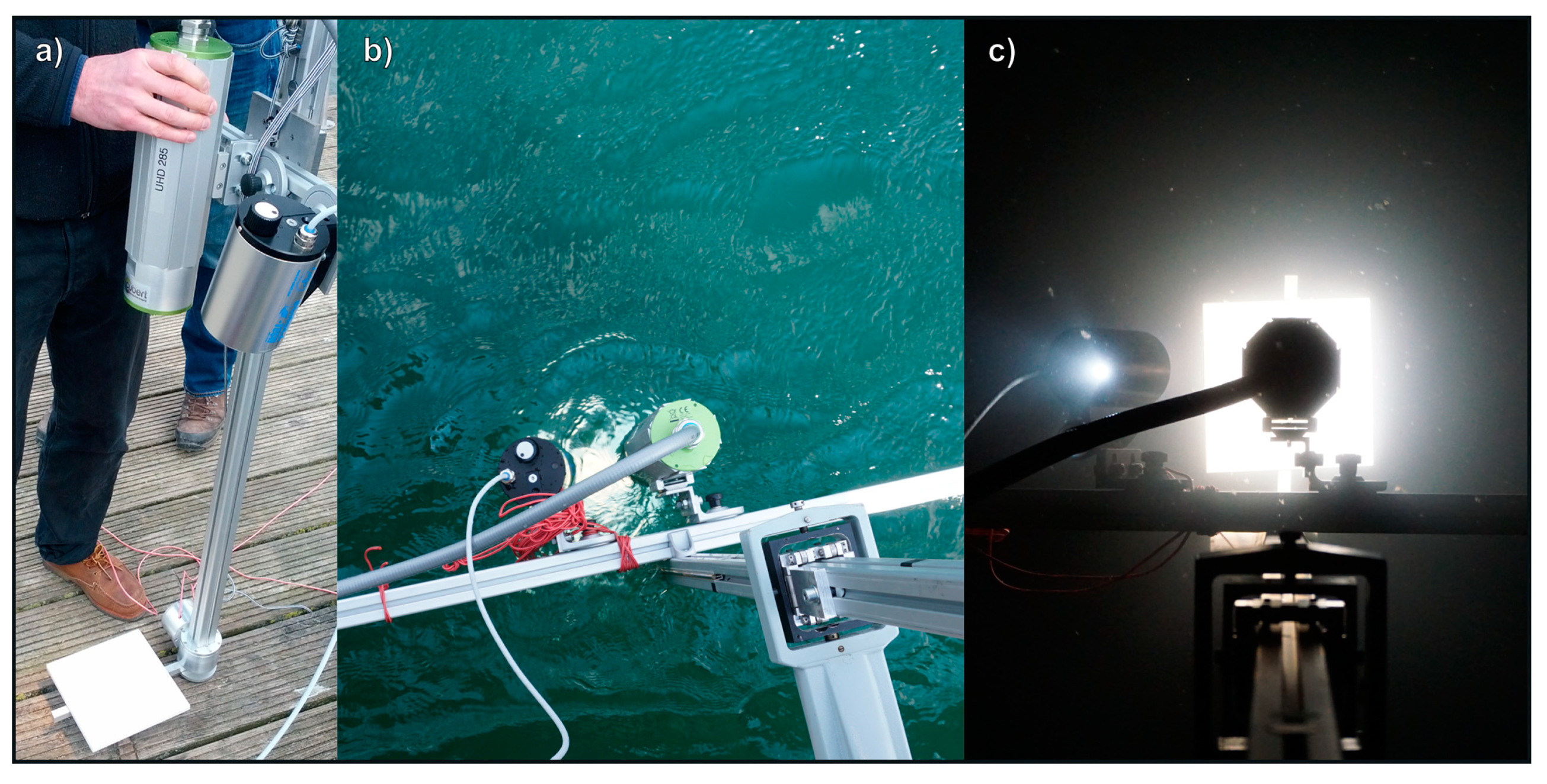
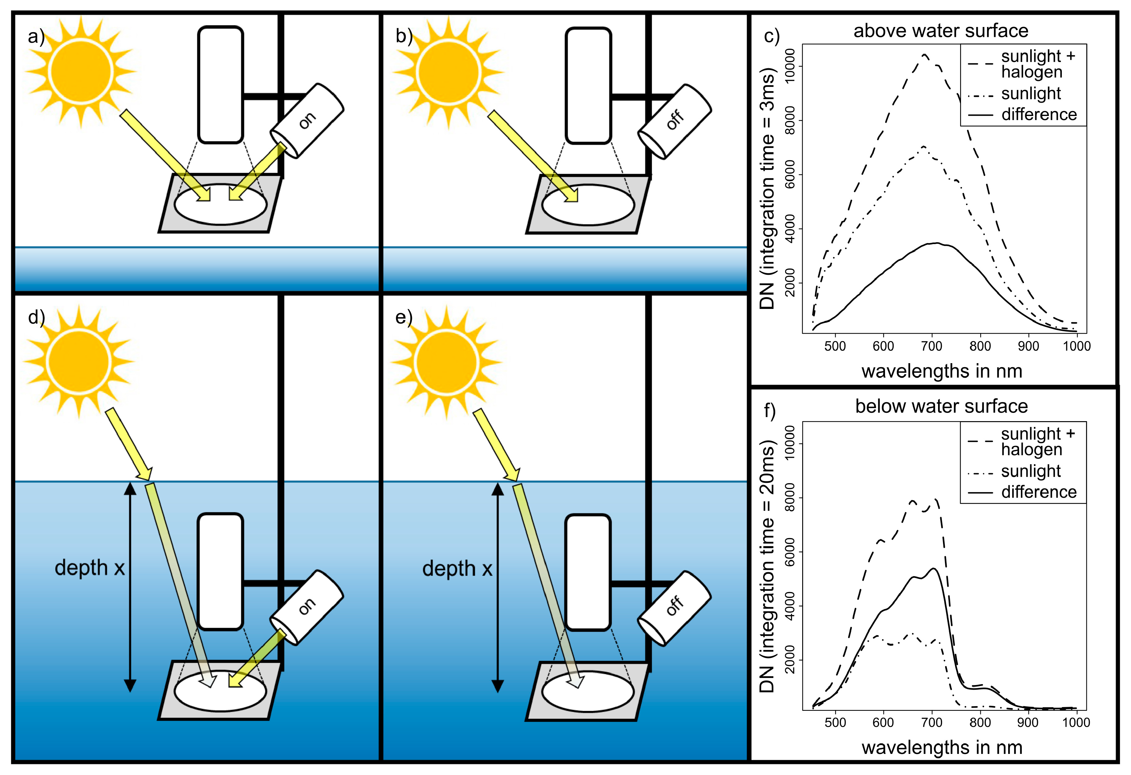
2.1. Hyperspectral Snapshot Camera

We collected hyperspectral measurements with a snapshot camera system (UHD 285; Cubert GmbH, Ulm, Germany) incorporated in a waterproof casing. The camera used a silicon CCD chip, which enabled the simultaneous acquisition of an entire three-dimensional hyperspectral image cube with one trigger pull. Its built-in sensor covered the spectral range of 450–998 nm with 8 nm spectral resolution at a 4 nm sampling interval. The acquired hyperspectral image cubes had a resolution of 50 x 50 pixels, resulting in 2500 spectra at 138 wavelengths. Due to spectral artifacts in the first few spectral bands and a Si-induced sensitivity loss at the end of the spectrum [28], we reduced the final spectral range to 470–850 nm with 96 spectral bands.

2.2. Laboratory Experiment

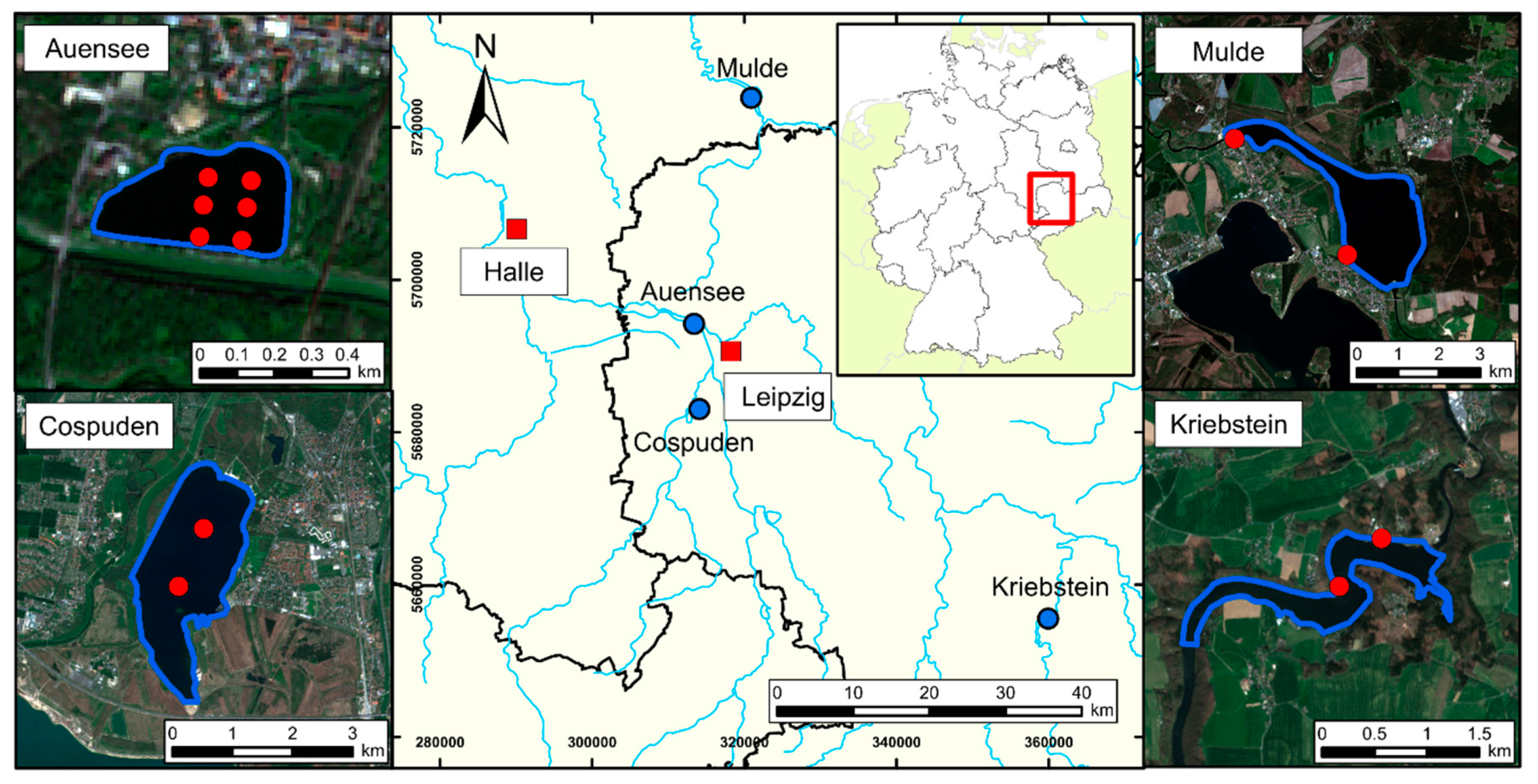
To test the camera’s ability to capture small changes in OAS contents, we compared its performance with parallel measurements using an ASD FieldSpec 4 (Malvern Panalytical Ltd., Almelo, The Netherlands) point spectrometer in a laboratory experiment.

The laboratory setup included a small water tank with a 20 × 20 cm Zenith Polymer^® (white panel with an average absolute reflectance of 0.95) placed at the bottom. Both spectrometers were installed with a nadir viewing geometry, and the scene was illuminated with an ASD ProLamp (14.5 V, 50 W) at a 45° zenith angle. After calibrating the instruments, we filled the tank with distilled water up to a column height of 20 cm. The ASD measurements were carried out directly above the water surface as the instruments’ fiber optics cable could not be immersed in the water. To exclude contributions to the measured radiance due to specular reflection at the air-water interface, the fibre optics cable was encased with a non-reflective material. The measured reflectance thus referred to the water-leaving radiance after passage through the interface:

$${\rho }_{ASD}=\frac{L_w}{L_{0,lamp}}$$

(1)

where $L_w$ is the water-leaving radiance and $L_{0,lamp}$ is the radiance of the light source at the water surface, measured through the reference panel.

Measurements with the hyperspectral camera were carried out with the camera opening placed slightly below the water surface. The measured reflectance thus refers to the upwelling underwater radiance:

$${\rho }_{Cam}=\frac{L_u}{L_{0,lamp}}$$

(2)

where $L_u$ is the upwelling radiance before transmission through the surface.

The two reflectances can be related through a dimensionless proportionality factor that accounts for the transmission through the water–air interface [29]. Since we were mainly interested in the quality of the camera’s data acquisition, i.e., shape of reflectance spectra, resolution of peaks, signal-to-noise ratio, and also carried out the field measurements (Section 2.5) below the water surface, we decided not to convert the ASD spectra to camera-equivalent reflectances.

We carried out two separate series of measurements to test the spectral response of CDOM and CHLa. Humic acid-sodium salt and a commercial Chlorella sp. powder were used as surrogates for CDOM and CHLa, respectively. Both substances were each mixed into the tank’s water at increasing concentrations (CDOM with absorption coefficients at 440 nm: 0.0–0.5 m⁻¹ in 0.1 increments, and 0.5–3.0 m⁻¹ in 0.5 increments; CHLa: 0.0–12.5 µg L⁻¹ in 2.5 increments, and 12.5–112.5 µg L⁻¹ in 12.5 increments) and reflectance spectra were recorded at each stage.

2.3. Field Campaign

For the field campaign, we investigated four artificial freshwater lakes in Central Germany (Figure 1), which were characterized by significant differences in size, trophic state index, and management practices (

Table 1. Characteristics of the investigated lake sites in Central Germany.

Site	Area (ha)	Trophic State Index	Type	Secchi Depth * (m)	Number of Sampling Points	Number of Sampling Units
Auensee	12	Eutrophic/hypereutrophic	Former gravel pit	0.40–0.65	6	27
Cospuden	436	Oligotrophic	Former open cast mine	6.00–6.05	2	10
Kriebstein	132	Oligotrophic	Reservoir	2.35–2.45	2	10
Mulde	630	Mesoeutrophic	Reservoir	1.25–1.30	2	9

* Refers to the viewing depth at the time of measurement using a 20 cm Secchi disk.

). The studied lakes were selected to cover a broad range in terms of depths of visibility, OAS concentrations and trophy with the aim to test the camera’s image acquisition and CHLa and CDOM modelling capabilities in different environments (Section 2.6). The shallow, hypereutrophic lake Auensee is a flooded, groundwater-fed former gravel pit with an average depth of 3.5 m, located in an inner city hardwood floodplain forest [30]. The groundwater-fed Cospuden Lake, with a maximum depth of ~54 m, represents a former open cast lignite mine [31], currently used as a recreational area. The Mulde and Kriebstein sites are both reservoirs, fed by the Mulde and the Zschopau river, respectively.

At each lake, spectral measurements and reference samples were collected at near-shore sampling points accessible by footbridges and at fixed markings within the lakes (Figure 1). Additionally, we determined the viewing depth using a 20 cm Secchi depth at each sampling point. For the Mulde, Kriebstein and Cospuden sites, measurements were carried out at two sampling points in each lake; whereas for the more variable Auensee site, samples were collected at six sampling points. Measurements were carried out for up to five continuous 0.5 m segments from the water surface down to a depth of 2.5 m, if possible, and for four segments in shallower waters. In total, 56 samples were taken.

2.4. CHLa and CDOM Reference Analysis

In parallel with the spectral measurements of the water column, we collected bulk water samples for each segment with a Ruttner water sampler (1.7 l, height: 24.5 cm). The samples were stored in cooling boxes and transported to the laboratory on the same day for the analysis of chlorophyll a (CHLa) and colored dissolved organic matter (CDOM). CHLa absorption was determined photometrically after hot ethanol extraction by using a SPECORD double-beam photometer with pure water (Milli-Q) as reference; CHLa concentrations were calculated afterwards according to ISO 10620 [32]. CDOM contents were also determined photometrically after filtering subsamples through Whatman GF/F-filters (pore size of 0.45 µm). The remaining filtrate was used to measure the absorbance of CDOM at 440 nm in 1 cm quartz cuvettes by using a SPECORD double-beam photometer with pure water (Milli-Q) as reference. Absorption coefficients were calculated according to the following expression [33]:

$$a_{CDOM}\left(440nm\right)=2.303·\frac{A\left(440nm\right)}{l}$$

(3)

where aCDOM(440 nm) is the CDOM absorption coefficient at 440 nm, A(440 nm) is the measured absorbance at 440 nm, and l is the path length of the cuvette in m.

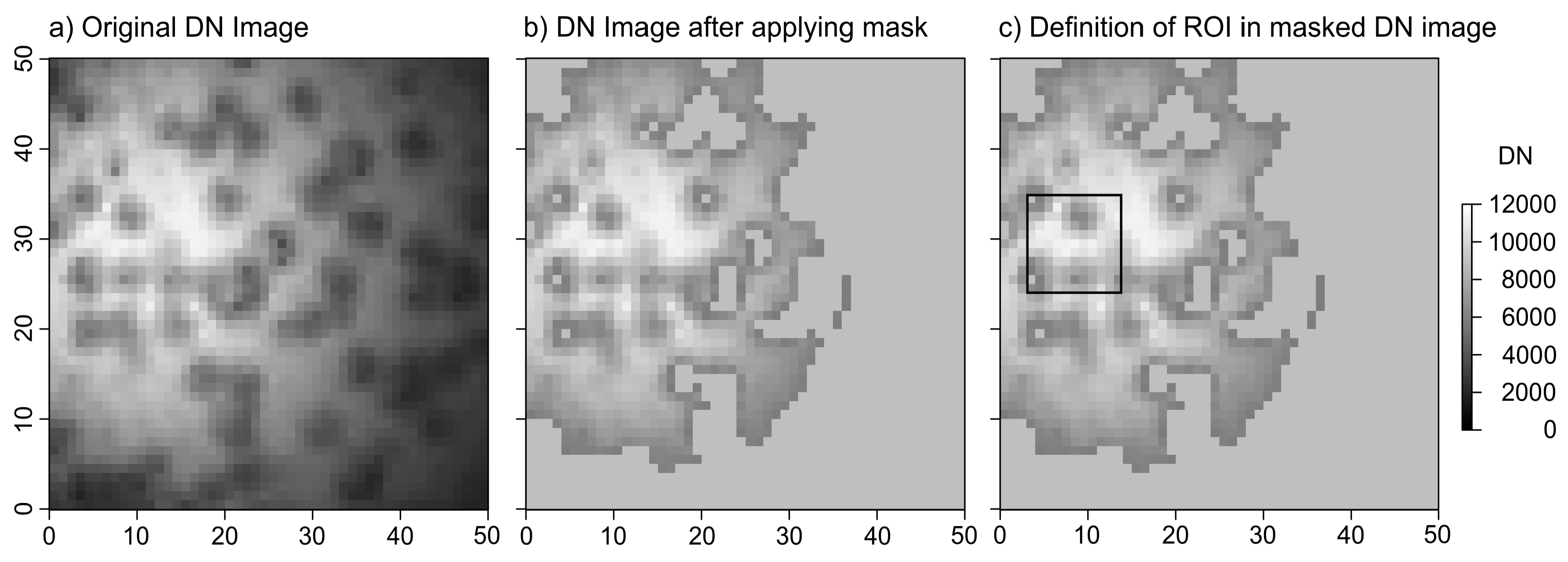
2.5. Hyperspectral Image Acquisition and Processing

For water column measurements, the hyperspectral camera system was mounted on a customized rack equipped with a portable halogen lamp (100 W). A Zenith Polymer^® reference panel (average absolute reflectance of 0.95; 25 × 25 cm) was attached in front of the camera at a fixed distance of 40 cm so that it covered the entire field of view of the camera (Figure 2).

Images of the reference panel above the water surface and of the individual water column segments were recorded in the raw digital number format (DN). Under optimal illumination conditions, the conversion from DN to radiance is a linear function and reflectance values can be calculated as:

$${\rho }_{sample}=\frac{D{N}_{sample}}{D{N}_{ref}}·{\rho }_{ref}·\left(\frac{t_{ref}}{t_{sample}}\right)$$

(4)

where ${\rho }_{sample}$ = reflectance of sample, DN = digital number, ${\rho }_{ref}$ = reflectance factor of the reference panel and t = integration time during the measurement.

At each sampling point, we measured the reference panel above the water surface to acquire a calibration file for the entire water column. Since ambient illumination varies for each measured segment due to non-linear sunlight attenuation through the water column, we compensated for this effect through parallel measurements of the reflectance target with and without artificial illumination to retrieve the final reflectance curves. That is, two separate images were taken for each measurement, both for the reference panel above the water surface and for the individual segments within the water column. The first image was taken with the external lamp switched on, the second image with the lamp switched off. The difference between the two respective images then represents the signal of the measured water column segment without the impact of ambient stray light (Figure 3). Before calculating the final mean reflectance spectrum, we performed two processing steps for each image (Figure 4) to define an optimally illuminated region within the image while minimizing the impact of interfering objects. First, we applied a binary mask by thresholding pixel values at 710 nm, the wavelength of maximum signal intensity of the halogen lamp. This wavelength yielded a high discrimination accuracy for the applied threshold due to an optimal signal-to-noise ratio and was also less influenced by absorption processes of our target variables (see Section 3.1).

Since the illumination conditions and OAS contents varied between the images, each image-specific threshold was defined as the mean DN value at 710 nm. All pixels with a DN value less than the image mean were discarded to remove poorly illuminated pixels and interfering image objects (e.g., shadowing effects of surface waves, bubbles due to gaseous emissions from the seafloor, or floating plant residues in the water column). In the second step, we defined a square region of interest (ROI) with a maximum of 121 pixels centered at the pixel with the largest DN value (710 nm) to calculate the mean DN spectrum for each image (Figure 4).

Finally, the reflectance of each water column segment was calculated from the extracted mean DN spectra as:

$${\rho }_{sample}=\frac{\overline{DN}{\left(x\right)}_{sun+lamp}-\overline{DN}{\left(x\right)}_{sun}}{\overline{DN}{\left(x=0\right)}_{sun+lamp}-\overline{DN}{\left(x=0\right)}_{sun}}·{\rho }_{ref}·\left(\frac{t_{x=0}}{t_x}\right)$$

(5)

where the numerator represents the averaged sunlight-compensated DN of the measurement at depth x, the denominator represents the averaged sunlight-compensated DN of the reference panel measured above the water surface (x = 0), and $t_x$ and $t_{x=0}$ are the corresponding integration times.

Accordingly, the calculated reflectance curves were only dependent on the energy input of the external halogen light source and were thus comparable across all investigated water bodies.

To validate the compensation algorithm, we compared the calculated reflectance curves of daytime and nighttime measurements at the Cospuden site. During nighttime measurements, ambient light does not interfere with the measurements, so that these measurements only reflect the contributions of the halogen light source. As the Cospuden site was oligotrophic, no additional OAS variability was expected to contribute to the spectral information. The shape of the spectral signatures was therefore expected to remain constant throughout the entire vertical profile, regardless of any daytime ambient light effects.

2.6. Predictive Modeling of CHLa and CDOM

Based on the aggregated field dataset, we tested two different empirical approaches to estimate CHLa and CDOM including two waveband indices for each target variable and multivariate regression based on the full spectrum. For CHLa, we used the following three-band ratio, which is widespread in remote sensing applications [34], see in [8]:

$$CHLa=a+b\left(\frac{1}{R_{670}}-\frac{1}{R_{710}}\right)·R_{750}$$

(6)

where a and b are model coefficients that were empirically re-optimized in the cross-validation loop, R is reflectance, and the subscript indicates the wavelength in nm. Additionally, we applied a single waveband model based on the first derivative of the reflectance signal at 690 nm, shown to work well for CHLa estimation in reservoirs by [35]:

$$CHLa=a+b\left({R^{\prime }}_{690}\right)$$

(7)

where R′ is the first derivative of the reflectance curve.

For CDOM, we used a published two-band ratio model [36], which was tested successfully at various lakes by Zhu et al. (2014) [37]:

$$CDOM=a{\left(\frac{R_{570}}{R_{654}}\right)}^b$$

(8)

The choice between existing CDOM algorithms was limited to the spectral range we used for our dataset (470–850 nm) since many of the empirical algorithms are based on wavelengths <470 nm [37]. In parallel to the approach of [35] for CHLa, we empirically defined the wavelength at 602 nm as the one with the strongest correlation between CDOM and the first derivative of reflectance, resulting in the following model:

$$CDOM=a+b\left({R^{\prime }}_{602}\right)$$

(9)

To compare the performance of target variable-specific waveband indices with the use of hyperspectral data, we calibrated partial least squares regression (PLSR) models [38] with reflectance (PLS_ref) and first derivative spectra (PLS_fda) using the full spectral range. PLSR is widely used in chemometrics to develop multivariate calibrations with hyperspectral data. The method can cope with multicollinear and noisy datasets and has been applied in hyperspectral water spectroscopy of optically complex waters where OAS specific empirical band ratios might produce inaccurate results (e.g., [39,40,41,42]).

All models were evaluated with a ‘leave-one-profile-out’ cross-validation (CV). Therefore, we split the entire dataset iteratively up into eleven water column profiles for calibration, applying either the above-mentioned waveband models or full range PLSR, and the remaining water column profile for validation. Subsequently, we pooled the estimates of the individually cross-validated profiles for each method and calculated the following performance measures to evaluate the models: coefficient of determination (R²), root mean square error (RMSE):

$$RMSE=\sqrt{\frac{\sum {\left(\hat{\mathrm{y}}-y\right)}^2}{n}}$$

(10)

where y = measured value, $\hat{\mathrm{y}}$ = estimated value and n = number of samples, and the ratio of performance to interquartile range (RPIQ):

$$RPIQ=\frac{IQR}{RMSE}$$

(11)

where IQR is the interquartile range of the reference data.

3. Results and Discussion

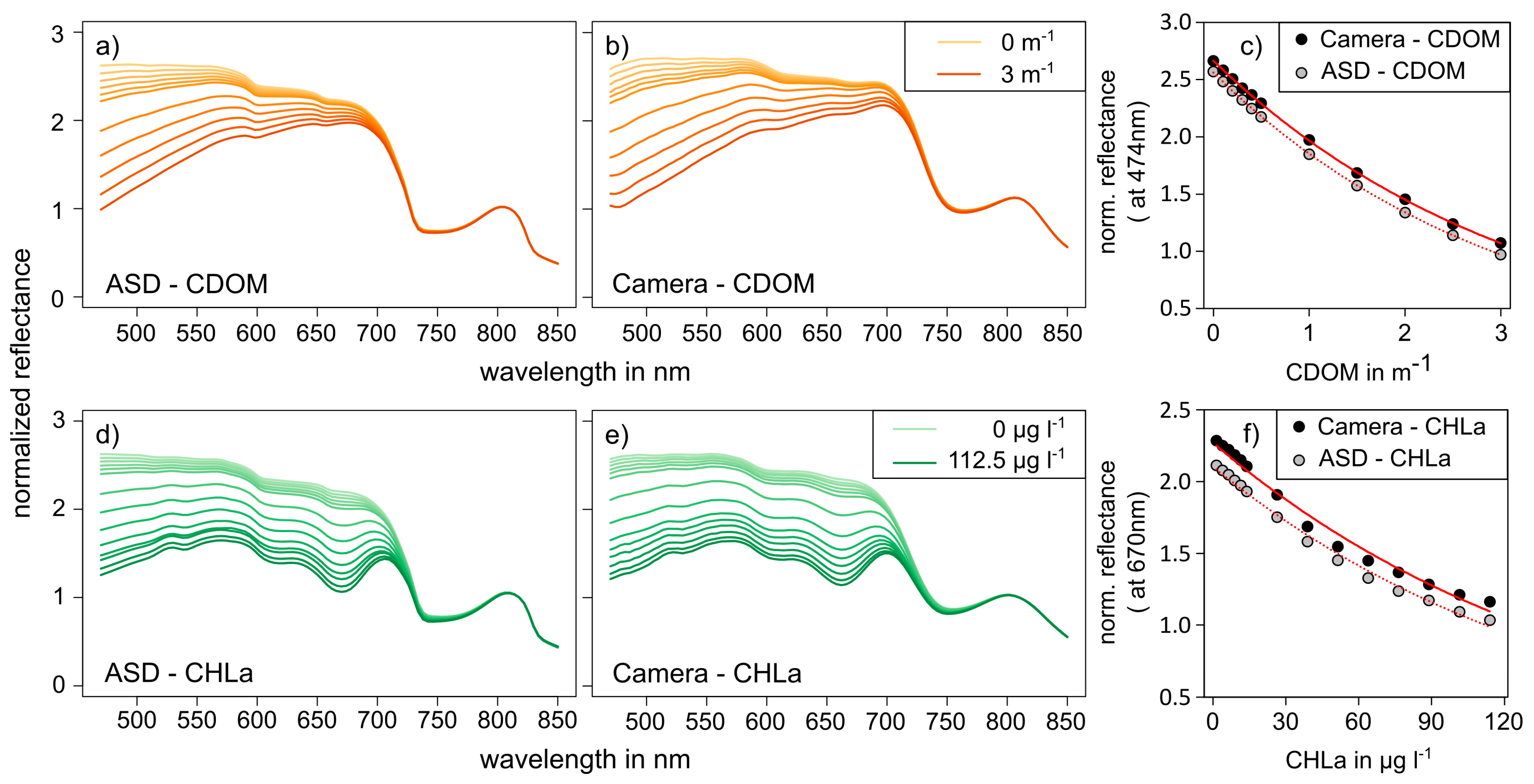
3.1. Laboratory Experiment

The results of the performed laboratory experiments are summarized in Figure 5. For reasons of comparison with the hyperspectral camera, we reduced the ASD spectra to a range between 470 and 850 nm. Additionally, we normalized all spectra to the measured reflectance at 810 nm to minimize potential scattering effects due to particulate characteristics of the added substances. The spectra recorded with the UHD 285 hyperspectral camera and the ASD FieldSpec point spectrometer were very similar overall. Reflectance patterns and absorption features at various levels of CDOM and CHLa were clearly defined and did not show any significant deviations between the instruments. The minor systematic offset between the spectra of the point spectrometer and the hyperspectral camera was presumably a result of the measurement setup, as the front of the camera was positioned slightly below the water surface, in contrast to the fiber optic cable of the ASD spectrometer with a position just above the water surface. The addition of CDOM caused a gradual increase in absorption in the ‘blue-to-green’ spectral range (<550 nm) that leveled off at higher wavelengths as already described in previous studies (e.g., [43,44,45]). CDOM did not show any distinct absorption features in the VNIR range. The high absorption in the shorter wavelengths presumably reflected large absorption features of dissolved organic matter (DOM) in the ultraviolet (UV) range that tailed off in the VIS [43]. Increasing the concentrations of algae showed a more differentiated effect on the spectra with a characteristic CHLa absorption feature around 670 nm, but induced also less pronounced peaks around 620 nm and 540 nm that might have originated from accessory pigments of Chlorella sp.

The normalization of the reflectance spectra to the wavelength at 810 nm resulted in an almost perfect match of the spectral signatures at wavelengths longer than 710 nm. This documented that both substances were not spectrally active in this range. On the other hand, both substances showed overlaps in the entire range below 710 nm. Hence, the presence of one substance might impair the spectral retrieval of the other substance, leading to a non-unique solution referred to as the ill-posed problem of spectra analysis [46]. Besides the absorption coefficient at a certain wavelength in the 400–460 nm range, CDOM could also be characterized by the spectral slope that describes the exponential decay of CDOM absorbance with increasing wavelength and which strongly depends on the molecular composition of DOM (see [43]). The reference analysis in the performed experiment with dissolved humic acid in the given concentration range indeed revealed a spectral slope of 0.008 in the 400–500 nm range. In freshwater lakes, however, the spectral slope of CDOM typically varies in a range between 0.014 and 0.020 (see [44,45,47]), and therefore has a smaller impact on the ‘red’ spectral range at each given absorption coefficient. Nevertheless, high amounts of CDOM with typical values of the described spectral slope might also affect empirical algorithms for CHLa retrieval in optically complex waters if based on wavelengths around the CHLa feature at 670 nm.

In summary, the hyperspectral camera was able to capture small OAS variabilities with an accuracy comparable to the ASD point spectrometer under laboratory conditions. The signal quality of the image mean was comparable to the point measurement of the ASD instrument and the minor divergence in total reflectance resulted from differences in the instrumental setup.

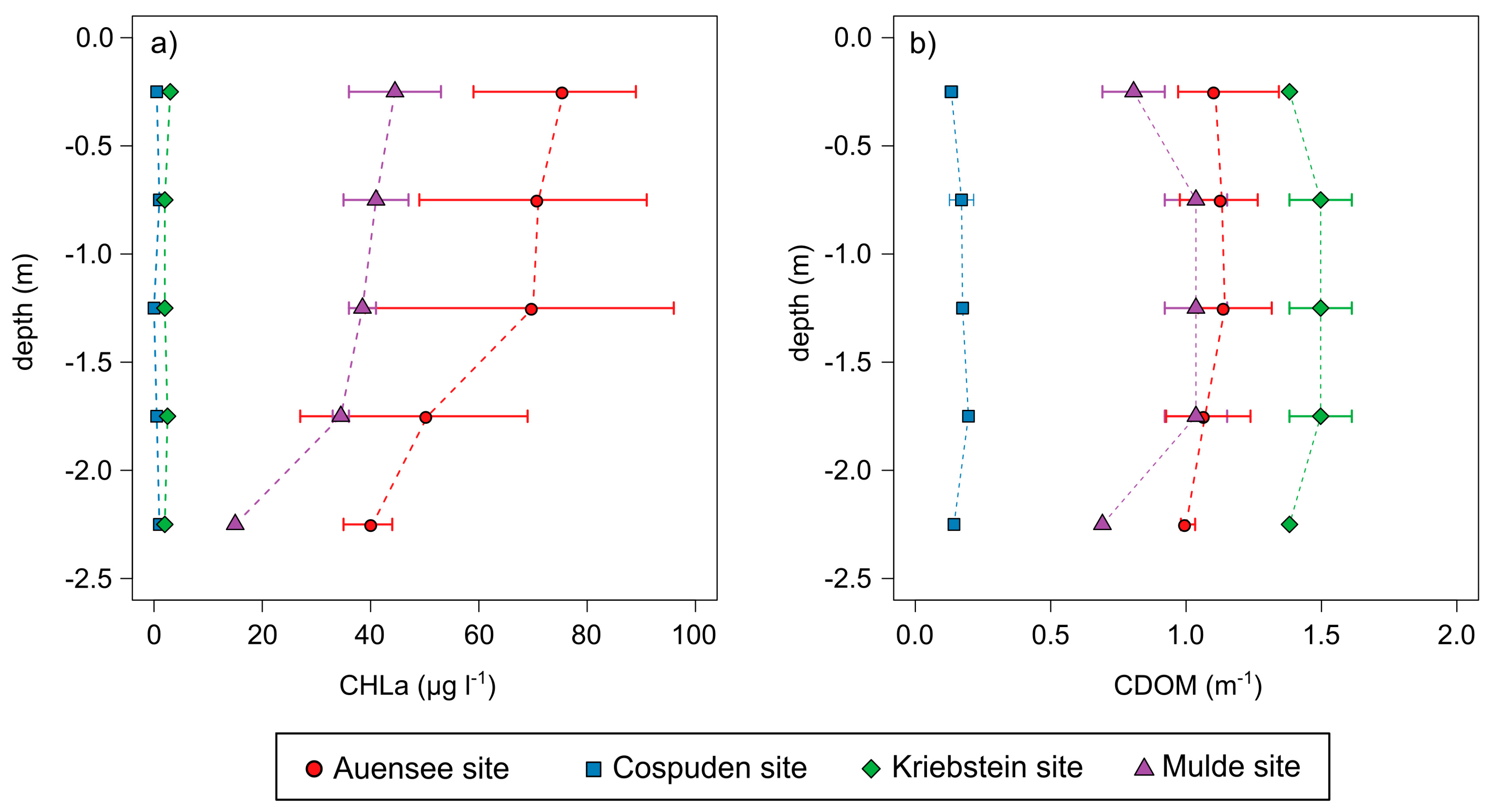
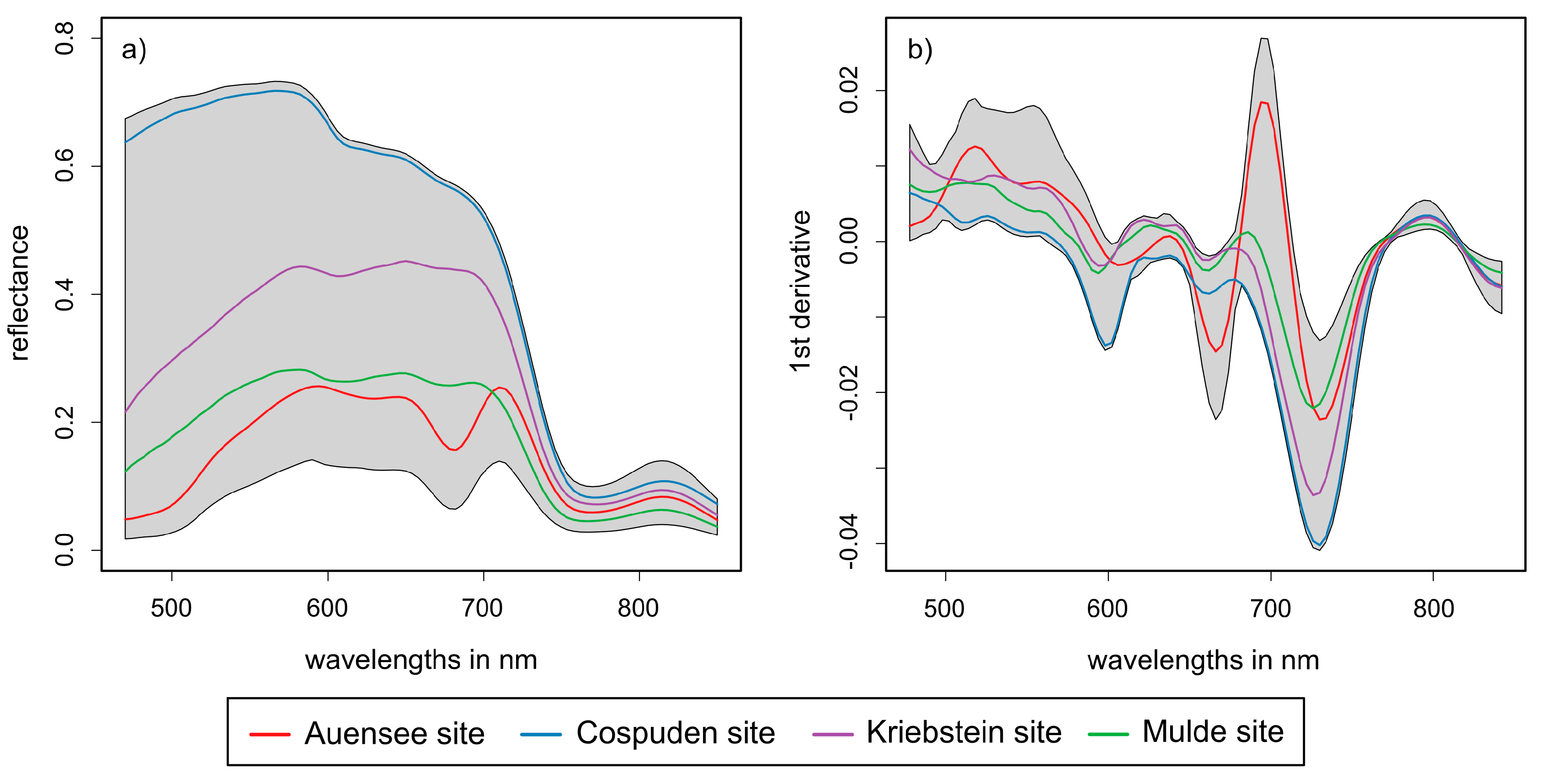
3.2. Water Quality Characteristics of the Investigated Lakes

The two target variables showed a high degree of variability between the studied lakes (see

Table 2. Descriptive Statistics of reference values of chlorophyll a—contents (CHLa, in µg L⁻¹) and CDOM absorbance at 440 nm (in m⁻¹). OAS = optically active substance, n = number of samples, min = minimum, Q1 = first quartile, Q2 = median, Q3 = third quartile, max = maximum, mean = arithmetic mean, sd = standard deviation.

OAS	Site	n	Min	Q1	Q2	Q3	Max	Mean	sd
CHLa	all	56	0	2	37	64	96	37.2	32.2
	Auensee	27	27	46	64	84	96	63.9	20.9
	Cospuden	10	0	0	1	1	1	0.6	0.5
	Kriebstein	10	2	2	2	3	3	2.3	0.5
	Mulde	9	15	35	36	41	53	36.9	10.5
CDOM	all	56	0.1	0.9	1.0	1.3	1.6	0.97	0.43
	Auensee	27	0.9	1.0	1.0	1.2	1.3	1.10	0.12
	Cospuden	10	0.1	0.1	0.2	0.2	0.2	0.16	0.03
	Kriebstein	10	1.4	1.4	1.4	1.6	1.6	1.45	0.11
	Mulde	9	0.7	0.9	0.9	1.2	1.2	0.95	0.18

). The CHLa contents of the complete dataset varied between 0 and 96 µg L⁻¹, with an overall mean concentration of 37.2 µg L⁻¹. The Cospuden and Kriebstein sites generally had low CHLa contents throughout the complete measured water column with site-specific mean values of 0.6 µg L⁻¹ and 2.3 µg L⁻¹, respectively, and a standard deviation of 0.5 µg L⁻¹. In the other two lakes mean concentrations were significantly higher with 63.9 µg L⁻¹ at the Auensee site and 36.9 µg L⁻¹ at the Mulde site.

A vertical CHLa stratification occurred in those lakes with relatively high CHLa contents (Figure 6). At the Auensee site, the layer-specific CHLa means ranged between 70 and 76 µg L⁻¹ within the upper 1.5 m, and the upper layers were also characterized by a high variability (indicated by wide ranges within each layer). By contrast, the average concentration dropped to almost half (40 µg L⁻¹) at a depth of 2.5 m. A similar pattern was observed at the Mulde site with mean values between 38 and 45 µg L⁻¹ in the upper 1.5 m and 15 µg L⁻¹ in the lowest layer. Due to the overall low CHLa contents, no substantial stratification was observed at the Cospuden and Kriebstein sites.

The results of the CDOM analysis showed less variability across the lakes with CDOM values between 0.1 and 1.6 m⁻¹. We found the lowest CDOM levels at the Cospuden site with a maximum absorption coefficient of 0.2 m⁻¹, whereas the remaining lakes showed mean levels between 0.95 at the Mulde site and 1.45 m⁻¹ at the Kriebstein site. In all four lakes, the vertical profile of CDOM showed an approximately uniform distribution.

In line with the relatively high CHLa concentrations in the surface layer, the Auensee site and the Mulde site showed the lowest Secchi disk depths measured during the field campaigns with ~0.5 m and ~1.3 m, respectively. Given that the Secchi depth approximates the water depth suitable for above-ground remote or proximal sensing, this documents the need for underwater in situ measurements to assess the complete vertical distribution of OAS.

3.3. Validation of Ambient Light Compensation

To validate the applicability of Equation (5) under realistic conditions, we compared the measured reflectance values of nighttime measurements at the Cospuden site with the calculated reflectance values of daytime measurements carried out only a few hours later at the same position (Figure 7).

The spectra of the nighttime measurements were almost identical for all five increments. The reflectance curves showed no variability in terms of OAS absorption features (Figure 7a), which was in line with the results of the laboratory reference analysis, as the entire water column showed negligible contents of CHLa and CDOM. The calculation of reflectance based on daytime measurements without sunlight compensation (Equation (4)) resulted in an increased spectral variability throughout the entire spectral range (Figure 7b). This was solely caused by varying conditions of the ambient light field with increasing water depth. Accordingly, the application of the sunlight compensation algorithm (Equation (5)) removed these differences almost entirely (Figure 7c) and implied an optimization for the retrieval of CDOM and CHLa at different depths, as both absorb in the affected wavelength ranges (as shown in Section 3.1).

At the Auensee site, with a Secchi depth of ~0.5 m, the measured signal below a depth of ~2 m was very low, even with greatly increased integration times, and the retrievable spectral information was therefore limited to the range between 500–700 nm (data not shown), corresponding to the energy maximum of sunlight in the visible range. In the remaining parts of the spectrum, the signal was overlaid by dark current. The authors of [22] also reported a signal loss of >78 % for wavelengths longer than 620 nm within the first meter of a freshwater lake with noticeable algae and cyanobacteria contents. The use of a portable lamp, as shown in the present study, therefore allowed to compensate for the effects of sunlight attenuation and the associated signal loss with increasing depth. The combination of a constant light source and a reference panel at a fixed distance in front of the camera simulated shallow water with a standardized bottom and resulted in almost constant measurement conditions throughout the entire water column. Consequently, all acquired reflectance spectra were comparable between the investigated lakes and across different depths.

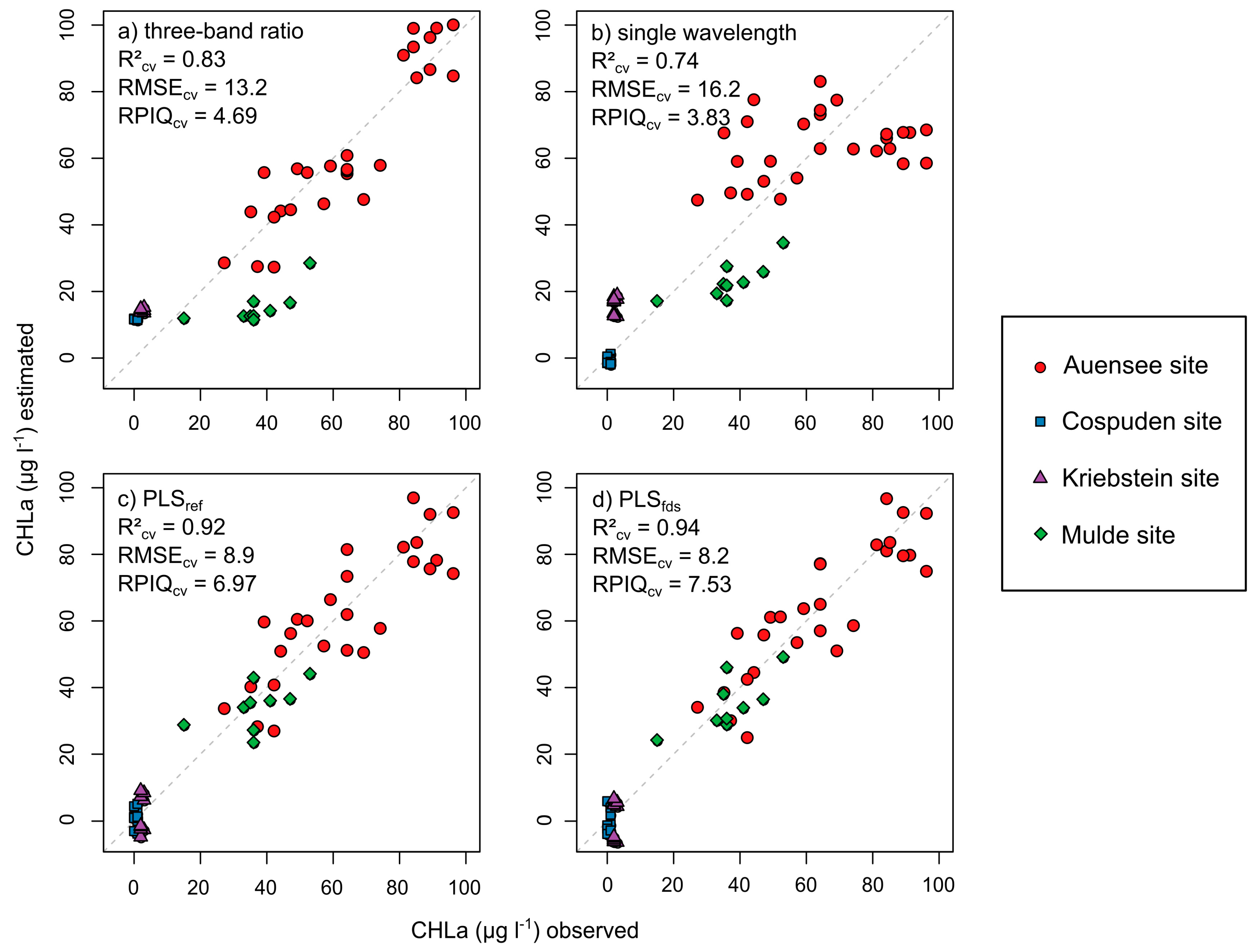
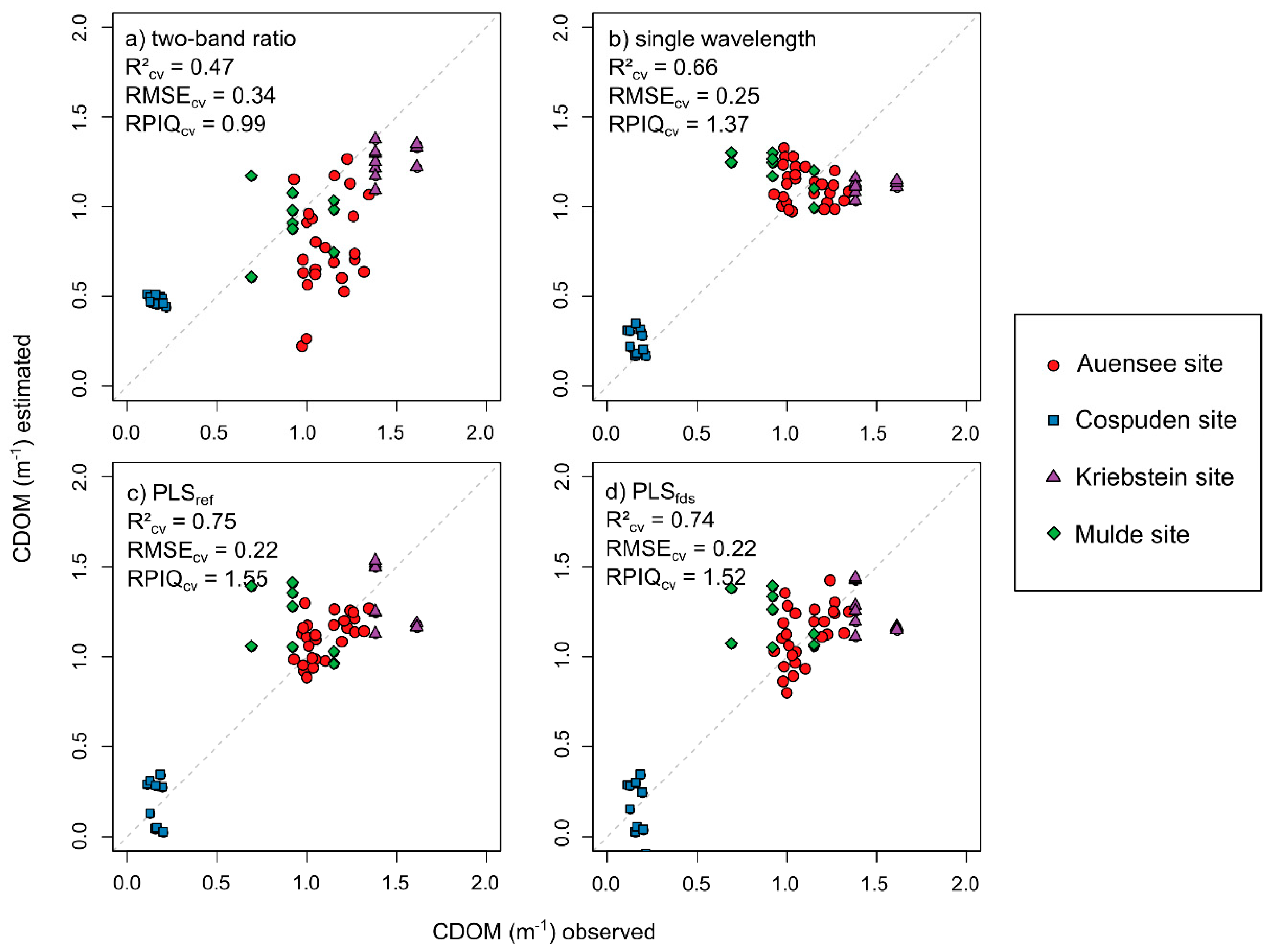
3.4. Predictive Modeling of CHLa and CDOM

The lake specific mean reflectance spectra (Figure 8) mirrored the measured OAS reference values. Starting with the mean spectrum of the Cospuden site, which represented low contents of CHLa and CDOM, a clear decrease of reflectance mainly at the shorter wavelengths was observed for the Kriebstein site, mainly attributable to high CDOM levels. Since CHLa was low, reduced reflectance values in the ‘red’ range might also be caused by CDOM at this site. Although CDOM absorption decays exponentially with increasing wavelengths, this finding suggests that high and variable CDOM contents may also affect CHLa retrieval based on the absorption feature at around 670 nm. The Auensee site showed the lowest overall reflectance curves due to both, high CDOM and CHLa contents, with a marked CHLa feature at ~670 nm. The application of the first derivative on the spectra resulted in the removal of the baseline and a narrowing of the reflective range especially in the region below 670 nm. Values at zero indicated pronounced peaks and troughs of the reflectance spectra, whereas slope differences were highlighted by the first derivative.

Based on the found spectral sensitivities, the three-band ratio model worked well for CHLa retrieval in the case of the eutrophic and turbid Auensee waterbody (

Table 3. Root mean square error (RMSE) (in µg L⁻¹) for CHLa estimation per lake.

Site	Three-Band Ratio	Single Wavelength	PLSref	PLSfds
Auensee (63.9) *	9.52	19.86	11.24	10.29
Cospuden (0.6) *	11.04	1.72	2.69	3.46
Kriebstein (2.3) *	12.07	13.78	5.17	5.98
Mulde (36.9) *	22.78	15.23	8.72	7.13

* Values in parentheses represent measured CHLa mean concentrations (in µg L⁻¹) of the lakes.

, Figure 9), which confirmed the applicability of this index for turbid and productive waters (see [8]).

For the Mulde site, however, values of nearly all samples were underestimated; conversely, we found a general overestimation of values for the remaining two sites (Cospuden, Kriebstein) with low CHLa contents. The single waveband approach based on spectral values of the first derivative at 690 nm showed similar results for the Mulde and Kriebstein sites compared to the three-band ratio. However, more accurate and precise estimates were achieved for the oligotrophic Cospuden site, whereas values of Auensee site samples with high CHLa levels being greater than 70 µg L⁻¹ were all underestimated (Figure 9). For lakes with very low CHLa (and CDOM) concentrations, however, relative estimation errors, compared to the lake-specific mean values, were very large due to the small dynamic range in CHLa and CDOM. In the case of the Cospuden and Kriebstein sites, the water bodies were essentially transparent and the range of observed values was consequently lower than the sensitivity of the reflectance spectra given the uncertainties included in field measurements.

For all studied samples, the overall RMSE of cross-validation was 13.2 µg L⁻¹ (three-band ratio) and 16 µg L⁻¹ (single waveband), respectively. Similar results were found by Duan et al. (2010) [48] who investigated a single eutrophic lake and achieved slightly better results with the three-band ratio compared to the use of the single waveband of the first derivative at 680 nm. Nevertheless, Cheng et al. (2013) [49] showed that first derivative models using one waveband in the 690–700 nm range might be more robust when transferred to independent datasets compared to two-, three-, and four-band ratios of reflectance spectra.

With regard to the entire dataset, the PLSR models based on the full spectral information provided higher accuracies with RMSE values at 8.9 µg L⁻¹, and 8.2 µg L⁻¹, the latter for the first derivative (Figure 9). In addition, there was no systematic over- or under-estimation of a lake-specific sample set or a certain CHLa range. These results suggest that the use of full range reflectance in combination with an empirical multivariate model produces potentially more accurate and robust results than spectral indices, which is in line with other studies (e.g., [40,41,42]). The authors of [41], who combined PLSR with a genetic algorithm to identify most suitable CHLa sensitive wavelengths, emphasized a better transferability of models calibrated in that way to new sites compared to empirical models based on three-band indices. Nevertheless, the data in Table 3 indicate that CHLa related band indices may provide similarly good or even more accurate results at specific lakes compared to full spectrum approaches. However, prior expert knowledge of the lake under consideration seems to be necessary for the selection of a suitable index, as their estimation accuracies showed a higher variability between the lakes compared to the use of full spectrum models.

These findings suggest that the use of continuous hyperspectral data in the range between ~400 and ~1000 nm for CHLa retrieval is generally of advance compared to the use of band ratio models. Benefits relate to accuracy and transferability, especially for highly diverse water bodies or multiple water bodies with variable conditions.

For CDOM, the results were different (

Table 4. RMSE (in m⁻¹) for CDOM estimation per lake.

Site	Two-Band Ratio	Single Wavelength	PLSref	PLSfds
Auensee (1.10) *	0.42	0.18	0.11	0.15
Cospuden (0.16) *	0.32	0.12	0.17	0.16
Kriebstein (1.45) *	0.22	0.35	0.27	0.27
Mulde (0.95) *	0.23	0.36	0.38	0.36

* Values in parentheses represent measured CDOM mean levels (in m⁻¹) of the lakes.

, Figure 10), which may be traced back to strong influences of e.g., algal biomass on the main region of CDOM absorption in the visible domain (see Section 3.1). Regarding the lake-specific error metrics (Table 4), the indices again show a variable pattern of estimation accuracies. While the single wavelength approach based on the first derivative value at 602 nm achieved the most consistent result of all models for the Cospuden site, the most accurate estimations for the Mulde site were yielded by the two-band ratio. Full spectrum models provided their best results for the Auensee and Cospuden sites.

Overall estimation accuracies, as indicated by RPIQ values (Figure 10), were thus significantly lower than those for CHLa. The two-band ratio approach produced the poorest results. This contrasts to Zhu et al. (2014) [37], who achieved—with this index—RMSE values at 0.28 m⁻¹ for lakes with CDOM levels between 0.9 and 2.1 m⁻¹ and at 0.05 m⁻¹ for CDOM levels beyond 3.4 m⁻¹. Nevertheless, they also stated that the algorithm might overestimate low CDOM levels. In our study, the single waveband index derived from the first derivative spectra outperformed the two-band ratio index. At this point, the physical relevance of the wavelength region at around 602 nm for the retrieval of CDOM is not obvious, but Brezonik et al. (2015) [47] also summarized several studies that included (at least with moderate success) wavelength regions beyond 500 nm for the retrieval of CDOM. Shao et al. (2016) [50] also tested different index approaches and found a ratio index calculated from reflectance values at 584 nm and 646 nm to outperform a single band index based on values of the first derivative at 406 nm (which showed the highest correlation with CDOM in their dataset). Additionally, they applied PLS with a back-propagation artificial neural network, but this provided less accurate results compared to the two-band ratio approach. Our results showed, different from that, that PLSR with both reflectance and first derivative spectra produced overall more accurate results with an RMSE at 0.22 m⁻¹. The plotted CDOM values revealed two clusters with markedly different levels of CDOM (which qualifies the applicability of one common linear approach and the retrieved statistical measures). Regardless of achieved estimation accuracies, the first derivative waveband approach and the PLS models were both able to separate these two classes, as evident from Figure 10.

Results for CDOM were generally poorer compared to CHLa, which might be due to a missing diagnostic absorption feature within the investigated spectral range of 470–850 nm and due to a large overlap between CDOM and CHLa absorption in the ‘blue’ spectral range. Additionally, further OAS such as detritus (non-living organic suspended matter), which is known to absorb in a similar pattern as CDOM does [51], may also affect CDOM retrieval. Therefore, accurate CDOM retrieval based on empirical methods seems to be still challenging, especially in optically complex waters.

Similar to our study, Abd-Elrahman et al. (2011) [26] also studied the retrieval of CHLa in fishery ponds by using a combination of hyperspectral measurements and submergible targets. To this end, they installed a hyperspectral scanner (400 to 1000 nm) above the water surface of 14 aquaculture ponds, where CHLa concentrations ranged from 0.8 to 494.4 µg L⁻¹. Additionally, they developed a three-level design of vertically arranged reflective targets. The first one was positioned above the water surface for calibration purposes, the second one 10 cm below, and the third one 30 cm below the water surface to test the effect of fixed viewing depths by using standardized bottoms. For CHLa retrieval, they used two-band and three-band indices. The best results were achieved with a three-band index and the target that was positioned 10 cm below the water surface (RMSE = 13.4 µg L⁻¹), whereas the lowest accuracy was obtained with the target 30 cm below the water surface (RMSE = 89.9 µg L⁻¹). They confirmed the advantage of using reflective targets in the upper water column to enhance the quality of the spectral signal. We successfully extended that approach by measuring multiple depths of 2.5 m water columns while being almost independent from ambient illumination conditions.

Generally, our results imply a strong potential for resolving the vertical water column at a fine scale for the provision of both, hyperspectral information and OAS products, which could be helpful for modelling approaches regarding the water leaving spectrum [15,16,52] and additionally provides insights into water layers below the viewing depth of above-ground remote or proximal sensors. Further, our measurement protocol proposes an experimental approach to cope with variable illumination conditions in order to obtain consistent reflectance spectra, which can be a critical aspect for in situ measurements [53]. The combination of its use for above-water surface measurements (e.g., [21,26]) and for underwater use (this study), hyperspectral cameras provide a potential link between point source underwater measurements and spectral imaging above the water surface.

4. Conclusions

We evaluated the performance of a submersible hyperspectral camera for underwater reflectance measurements and the estimation of CHLa and CDOM at various depths in four freshwater lakes with different trophic levels. The measurement configuration we developed allows a consistent retrieval of reflectance spectra throughout the water column with potential applications in OAS retrieval or radiometric ground truthing for remote sensing observations of the uppermost water layer. The available image information allows a pixel-wise analysis of the sensor’s field of view to improve data quality through the removal of poorly illuminated areas or interfering objects. For quantitative OAS retrieval, predictive models based on hyperspectral reflectance data can achieve more robust and accurate estimates for CHLa and CDOM than empirical algorithms based on specific wavebands, at least in complex datasets that include multiple lakes at different trophic levels. As our comparison included only two common waveband indices, however, a lake-specific selection of different band ratios might yield similar results to hyperspectral algorithms.

While the UHD 285 camera used in this study is a commercial-grade instrument with a mature data acquisition and processing chain, the customizations for underwater use, including the camera mount and the required instrument calibration procedures, were at a research level. Further refinements in the technology are necessary to allow a more rapid deployment, data acquisition and analysis, e.g., for near-real time water monitoring, the integration in sensor networks or operational use by environmental agencies.

Despite these present and future challenges, hyperspectral measurements throughout the water column may potentially bridge the gap between spatially continuous remote sensing observations of the surface water layer and point sensors that can provide continuous water monitoring data at and below the surface.

References

1. Aylward, B.; Bandyopadhyay, J.; Belausteguigotia, J.-C.; Börkey, P.; Cassar, A.; Meadors, L.; Saade, L.; Siebentritt, M.; Stein, R.; Tognetti, S.; et al. Freshwater ecosystem services. In Millenium Ecosystem Assessment: Ecosystems and Human Well-Being: Policy Responses; Chopra, K., Leemans, R., Kumar, P., Simons, H., Eds.; Island Press: Washington, DC, USA, 2005; pp. 213–255. [Google Scholar]
2. Schallenberg, M.; de Winton, M.D.; Verburg, P.; Kelly, D.J.; Hamill, K.D.; Hamilton, D.P. Ecosystem services of lakes. In Ecosystem Services in New Zealand–Conditions and Trends; Dymond, J.R., Ed.; Whenua Press: Lincoln, New Zealand, 2013; pp. 203–225. [Google Scholar]
3. Carpenter, S.R.; Stanley, E.H.; Zanden, M.J.V. State of the World’s Freshwater Ecosystems: Physical, Chemical, and Biological Changes. Annu. Rev. Environ. Resour. 2011, 36, 75–99. [Google Scholar] [CrossRef] [Green Version]
4. Dörnhöfer, K.; Oppelt, N. Remote sensing for lake research and monitoring – Recent advances. Ecol. Indic. 2016, 64, 105–122. [Google Scholar] [CrossRef]
5. Gholizadeh, M.H.; Melesse, A.; Reddi, L.N. A Comprehensive Review on Water Quality Parameters Estimation Using Remote Sensing Techniques. Sensors 2016, 16, 1298. [Google Scholar] [CrossRef] [Green Version]
6. Odermatt, D.; Gitelson, A.; Brando, V.; Schaepman, M.E. Review of constituent retrieval in optically deep and complex waters from satellite imagery. Remote Sens. Environ. 2012, 118, 116–126. [Google Scholar] [CrossRef] [Green Version]
7. Giardino, C.; Brando, V.; Gege, P.; Pinnel, N.; Hochberg, E.; Knaeps, E.; Reusen, I.; Doerffer, R.; Bresciani, M.; Braga, F.; et al. Imaging Spectrometry of Inland and Coastal Waters: State of the Art, Achievements and Perspectives. Surv. Geophys. 2018, 40, 401–429. [Google Scholar] [CrossRef] [Green Version]
8. Matthews, M. A current review of empirical procedures of remote sensing in inland and near-coastal transitional waters. Int. J. Remote Sens. 2011, 32, 6855–6899. [Google Scholar] [CrossRef]
9. Palmer, S.; Kutser, T.; Hunter, P.D. Remote sensing of inland waters: Challenges, progress and future directions. Remote Sens. Environ. 2015, 157, 1–8. [Google Scholar] [CrossRef] [Green Version]
10. Matthews, M.; Bernard, S. Characterizing the Absorption Properties for Remote Sensing of Three Small Optically-Diverse South African Reservoirs. Remote Sens. 2013, 5, 4370–4404. [Google Scholar] [CrossRef] [Green Version]
11. Bernardo, N.; Watanabe, F.; Rodrigues, T.; Alcantara, E. Atmospheric correction issues for retrieving total suspended matter concentrations in inland waters using OLI/Landsat-8 image. Adv. Space Res. 2017, 59, 2335–2348. [Google Scholar] [CrossRef] [Green Version]
12. Moses, W.J.; Sterckx, S.; Montes, M.J.; Keukelaere, L.D.; Knaeps, E. Atmospheric correction for inland waters. In Bio-Optical Modeling and Remote Sensing of Inland Waters, 1st ed.; Deepak, M., Ogashawara, I., Gitelson, A., Eds.; Elsevier: Amsterdam, The Netherlands, 2017; pp. 69–100. [Google Scholar]
13. Mouw, C.B.; Greb, S.; Aurin, D.; Digiacomo, P.M.; Lee, Z.; Twardowski, M.; Binding, C.; Hu, C.; Ma, R.; Moore, T.; et al. Aquatic color radiometry remote sensing of coastal and inland waters: Challenges and recommendations for future satellite missions. Remote Sens. Environ. 2015, 160, 15–30. [Google Scholar] [CrossRef]
14. Sterckx, S.; Knaeps, E.; Ruddick, K. Detection and correction of adjacency effects in hyperspectral airborne data of coastal and inland waters: The use of the near infrared similarity spectrum. Int. J. Remote Sens. 2011, 32, 6479–6505. [Google Scholar] [CrossRef]
15. Kutser, T.; Metsamaa, L.; Dekker, A. Influence of the vertical distribution of cyanobacteria in the water column on the remote sensing signal. Estuar. Coast. Shelf Sci. 2008, 78, 649–654. [Google Scholar] [CrossRef]
16. Pitarch, J.; Odermatt, D.; Kawka, M.; Wüest, A. Retrieval of vertical particle concentration profiles by optical remote sensing: A model study. Opt. Express 2014, 22, A947–A959. [Google Scholar] [CrossRef] [PubMed]
17. Xue, K.; Zhang, Y.; Duan, H.; Ma, R.; Loiselle, S.A.; Zhang, M. A Remote Sensing Approach to Estimate Vertical Profile Classes of Phytoplankton in a Eutrophic Lake. Remote Sens. 2015, 7, 14403–14427. [Google Scholar] [CrossRef] [Green Version]
18. Xue, K.; Zhang, Y.; Ma, R.; Duan, H. An approach to correct the effects of phytoplankton vertical nonuniform distribution on remote sensing reflectance of cyanobacterial bloom waters. Limnol. Oceanogr. Methods 2017, 15, 302–319. [Google Scholar] [CrossRef]
19. Leach, T.H.; Beisner, B.; Carey, C.C.; Pernica, P.; Rose, K.C.; Huot, Y.; Brentrup, J.A.; Domaizon, I.; Grossart, H.-P.; Ibelings, B.W.; et al. Patterns and drivers of deep chlorophyll maxima structure in 100 lakes: The relative importance of light and thermal stratification. Limnol. Oceanogr. 2017, 63, 628–646. [Google Scholar] [CrossRef] [Green Version]
20. Duan, W.; He, B.; Chen, Y.; Zou, S.; Wang, Y.; Nover, D.; Chen, W.; Yang, G. Identification of long-term trends and seasonality in high-frequency water quality data from the Yangtze River basin, China. PLoS ONE 2018, 13. [Google Scholar] [CrossRef]
21. Keller, S.; Maier, P.M.; Riese, F.; Norra, S.; Holbach, A.; Börsig, N.; Wilhelms, A.; Moldaenke, C.; Zaake, A.; Hinz, S. Hyperspectral Data and Machine Learning for Estimating CDOM, Chlorophyll a, Diatoms, Green Algae and Turbidity. Int. J. Environ. Res. Public Heal. 2018, 15, 1881. [Google Scholar] [CrossRef] [Green Version]
22. Kwon, Y.S.; Pyo, J.; Duan, H.; Cho, K.H.; Park, Y.; Kwon, Y.-H. Drone-based hyperspectral remote sensing of cyanobacteria using vertical cumulative pigment concentration in a deep reservoir. Remote Sens. Environ. 2020, 236, 111517. [Google Scholar] [CrossRef]
23. Greb, S.; Odermatt, D.; Schaeffer, B.A.; Spyrakos, E.; Wang, M. Complementarity of in situ and satellite measurements. In Earth Observations in Support of Global Water Quality Monitoring; Greb, S., Dekker, A., Binding, C., Eds.; IOCCG: Dartmouth, NS, Canada, 2018; pp. 29–42. [Google Scholar]
24. Kutser, T.; Paavel, B.; Verpoorter, C.; Ligi, M.; Soomets, T.; Toming, K.; Casal, G. Remote Sensing of Black Lakes and Using 810 nm Reflectance Peak for Retrieving Water Quality Parameters of Optically Complex Waters. Remote Sens. 2016, 8, 497. [Google Scholar] [CrossRef]
25. Pyo, J.; Ligaray, M.V.; Kwon, Y.; Ahn, M.-H.; Kim, K.; Lee, H.; Kang, T.; Cho, S.B.; Park, Y.; Cho, K.H. High-Spatial Resolution Monitoring of Phycocyanin and Chlorophyll-a Using Airborne Hyperspectral Imagery. Remote Sens. 2018, 10, 1180. [Google Scholar] [CrossRef] [Green Version]
26. Abd-Elrahman, A.; Croxton, M.; Pande-Chettri, R.; Toor, G.S.; Smith, S.E.; Hill, J. In situ estimation of water quality parameters in freshwater aquaculture ponds using hyperspectral imaging system. ISPRS J. Photogramm. Remote Sens. 2011, 66, 463–472. [Google Scholar] [CrossRef]
27. Wagner, A.; Hilgert, S.; Kattenborn, T.; Fuchs, S. Proximal VIS-NIR spectrometry to retrieve substance concentrations in surface waters using partial least squares modelling. Water Supply 2018, 19, 1204–1211. [Google Scholar] [CrossRef]
28. Jung, A.; Vohland, M.; Thiele-Bruhn, S. Use of A Portable Camera for Proximal Soil Sensing with Hyperspectral Image Data. Remote Sens. 2015, 7, 11434–11448. [Google Scholar] [CrossRef] [Green Version]
29. Mobley, C.D. Estimation of the remote-sensing reflectance from above-surface measurements. Appl. Opt. 1999, 38, 7442–7455. [Google Scholar] [CrossRef]
30. Dunker, S.; Nadrowski, K.; Jakob, T.; Kasprzak, P.; Becker, A.; Langner, U.; Kunath, C.; Harpole, S.; Wilhelm, C. Assessing in situ dominance pattern of phytoplankton classes by dominance analysis as a proxy for realized niches. Harmful Algae 2016, 58, 74–84. [Google Scholar] [CrossRef]
31. Abel, A.; Michael, A.; Zartl, A.; Werner, F. Impact of erosion-transported overburden dump materials on water quality in Lake Cospuden evolved from a former open cast lignite mine south of Leipzig, Germany. Environ. Earth Sci. 2000, 39, 683–688. [Google Scholar] [CrossRef]
32. ISO 10260. Water Quality—Measurement of Biochemical Parameters—Spectrometric Determination of the Chlorophyll-A Concentration; International Organization for Standardization: Geneva, Switzerland, 1992. [Google Scholar]
33. Mannino, A.; Novak, M.G.; Nelson, N.B.; Belz, M.; Berthon, J.-F.; Blough, N.V.; Boss, E.; Bricaud, A.; Chaves, J.; del Castillo, C.; et al. Measurement protocol of absorption by chromophoric dissolved organic matter (CDOM) and other dissolved materials (DRAFT). In Inherent Optical Property Measurements and Protocols: Absorption Coefficient; Mannino, A., Novak, M.G., Eds.; IOCCG: Dartmouth, NS, Canada, 2019; pp. 22–27. [Google Scholar]
34. Gitelson, A.A.; Gritz, Y.; Merzlyak, M.N. Relationships between leaf chlorophyll content and spectral reflectance and algorithms for non-destructive chlorophyll assessment in higher plant leaves. J. Plant Physiol. 2003, 160, 271–282. [Google Scholar] [CrossRef]
35. Han, L.; Rundquist, D.C. Comparison of NIR/RED ratio and first derivative of reflectance in estimating algal-chlorophyll concentration: A case study in a turbid reservoir. Remote Sens. Environ. 1997, 62, 253–261. [Google Scholar] [CrossRef]
36. Ficek, D.; Zapadka, T.; Dera, J. Remote sensing reflectance of Pomeranian lakes and the Baltic. Oceanologia 2011, 53, 959–970. [Google Scholar] [CrossRef] [Green Version]
37. Zhu, W.; Yu, Q.; Tian, Y.; Becker, B.L.; Zheng, T.; Carrick, H.J. An assessment of remote sensing algorithms for colored dissolved organic matter in complex freshwater environments. Remote Sens. Environ. 2014, 140, 766–778. [Google Scholar] [CrossRef]
38. Wold, S.; Sjöström, M.; Eriksson, L. PLS-regression: A basic tool of chemometrics. Chemom. Intell. Lab. Syst. 2001, 58, 109–130. [Google Scholar] [CrossRef]
39. Ali, K.A.; Ortiz, J.D. Multivariate approach for chlorophyll-a and suspended matter retrievals in Case II type waters using hyperspectral data. Hydrol. Sci. J. 2015, 61, 200–213. [Google Scholar] [CrossRef]
40. Ryan, K.; Ali, K. Application of a partial least-squares regression model to retrieve chlorophyll-a concentrations in coastal waters using hyper-spectral data. Ocean Sci. J. 2016, 51, 209–221. [Google Scholar] [CrossRef]
41. Song, K.; Li, L.; Tedesco, L.; Li, S.; Duan, H.; Liu, D.; Hall, B.; Du, J.; Li, Z.; Shi, K.; et al. Remote estimation of chlorophyll-a in turbid inland waters: Three-band model versus GA-PLS model. Remote Sens. Environ. 2013, 136, 342–357. [Google Scholar] [CrossRef]
42. Wang, Z.; Kawamura, K.; Sakuno, Y.; Fan, X.; Gong, Z.; Lim, J. Retrieval of Chlorophyll-a and Total Suspended Solids Using Iterative Stepwise Elimination Partial Least Squares (ISE-PLS) Regression Based on Field Hyperspectral Measurements in Irrigation Ponds in Higashihiroshima, Japan. Remote Sens. 2017, 9, 264. [Google Scholar] [CrossRef] [Green Version]
43. Helms, J.; Stubbins, A.; Ritchie, J.D.; Minor, E.C.; Kieber, D.J.; Mopper, K. Absorption spectral slopes and slope ratios as indicators of molecular weight, source, and photobleaching of chromophoric dissolved organic matter. Limnol. Oceanogr. 2008, 53, 955–969. [Google Scholar] [CrossRef] [Green Version]
44. Strömbeck, N.; Pierson, D. The effects of variability in the inherent optical properties on estimations of chlorophyll a by remote sensing in Swedish freshwaters. Sci. Total Environ. 2001, 268, 123–137. [Google Scholar] [CrossRef]
45. Twardowski, M.S.; Boss, E.; Sullivan, J.M.; Donaghay, P.L. Modeling the spectral shape of absorption by chromophoric dissolved organic matter. Mar. Chem. 2004, 89, 69–88. [Google Scholar] [CrossRef]
46. Defoin-Platel, M.; Chami, M. How ambiguous is the inverse problem of ocean color in coastal waters? J. Geophys. Res. Space Phys. 2007, 112, 843. [Google Scholar] [CrossRef] [Green Version]
47. Brezonik, P.L.; Olmanson, L.G.; Finlay, J.C.; Bauer, M.E. Factors affecting the measurement of CDOM by remote sensing of optically complex inland waters. Remote Sens. Environ. 2015, 157, 199–215. [Google Scholar] [CrossRef]
48. Duan, H.; Ma, R.; Xu, J.; Zhang, Y.; Zhang, B. Comparison of different semi-empirical algorithms to estimate chlorophyll-a concentration in inland lake water. Environ. Monit. Assess. 2009, 170, 231–244. [Google Scholar] [CrossRef] [PubMed]
49. Cheng, C.; Wei, Y.; Sun, X.; Zhou, Y. Estimation of Chlorophyll-a Concentration in Turbid Lake Using Spectral Smoothing and Derivative Analysis. Int. J. Environ. Res. Public Heal. 2013, 10, 2979–2994. [Google Scholar] [CrossRef] [PubMed] [Green Version]
50. Shao, T.; Song, K.; Du, J.; Zhao, Y.; Liu, Z.; Zhang, B. Retrieval of CDOM and DOC Using In Situ Hyperspectral Data: A Case Study for Potable Waters in Northeast China. J. Indian Soc. Remote Sens. 2015, 44, 77–89. [Google Scholar] [CrossRef]
51. Babin, M.; Stramski, D.; Ferrari, G.M.; Claustre, H.; Bricaud, A.; Obolensky, G.; Hoepffner, N. Variations in the light absorption coefficients of phytoplankton, nonalgal particles, and dissolved organic matter in coastal waters around Europe. J. Geophys. Res. Space Phys. 2003, 108, 3211. [Google Scholar] [CrossRef]
52. Nouchi, V.; Odermatt, D.; Wüest, A.; Bouffard, D. Effects of non-uniform vertical constituent profiles on remote sensing reflectance of oligo- to mesotrophic lakes. Eur. J. Remote Sens. 2018, 51, 808–821. [Google Scholar] [CrossRef]
53. Göritz, A.; Berger, S.A.; Gege, P.; Grossart, H.-P.; Nejstgaard, J.C.; Riedel, S.; Röttgers, R.; Utschig, C. Retrieval of Water Constituents from Hyperspectral In-Situ Measurements under Variable Cloud Cover—A Case Study at Lake Stechlin (Germany). Remote Sens. 2018, 10, 181. [Google Scholar] [CrossRef] [Green Version]
Figure 1. Location of the lake sites in Central Germany and sampling points (red dots) for water column measurements (satellite imagery: Sentinel 2A - RGB – 432 (17/04/2019); coordinate system of the map: ETRS89/UTM zone 33N).
Remotesensing 12 01745 g001
Figure 2. Hyperspectral camera system for underwater measurements: (a) camera system mounted on a rack with halogen light source and reference panel; (b) in situ measurement of uppermost water layer (0–0.5 m); (c) top-down view of night-time measurement in the water column (0.5–1.0 m).
Remotesensing 12 01745 g002
Figure 3. Field measurement setup for underwater reflectance retrieval: the upper row shows radiance measurements on the reference panel for calibration with light source turned on (a) and turned off (b). The difference of (a) and (b) represents the signal contributed by the light source only, which was used for instrument calibration (c). The lower row shows measurements below the water surface with the light source turned on (d) and turned off (e). The difference between measured spectra in configuration of (d) and (e) represents the reflected signal that only refers to the illumination from the artificial light source (f).
Remotesensing 12 01745 g003
Figure 4. Image processing steps to extract optimal mean spectra for multivariate calibrations: (a) example of 2D image (at 710 nm) recorded near the bottom of the Auensee site where suspended particles and bubbles appeared during image acquisition; (b) masking of poorly illuminated image areas and interfering elements; (c) definition of a region of interest (ROI) around the ‘brightest’ pixel (at 710 nm).
Remotesensing 12 01745 g004
Figure 5. Comparison of experimental laboratory measurements between ASD FieldSpec 4 and UHD 285 hyperspectral camera at various levels of colored dissolved organic matter (CDOM) (a,b), and chlorophyll a (CHLa) (d,e) concentrations. Panels (c,f) show a direct comparison of the measured reflectance at specific key wavelengths sensitive to changes in CDOM and CHLa, respectively.
Remotesensing 12 01745 g005
Figure 6. Vertical distribution of CHLa (a) and CDOM (b) for the investigated lake sites. Points mark the layer-specific mean, solid lines mark the layer-specific range of measured reference values.
Remotesensing 12 01745 g006
Figure 7. Comparison of reflectance spectra acquired at Cospuden site during (a) nighttime measurements, (b) daytime measurements without compensation for sunlight attenuation, and (c) daytime measurements with compensation for sunlight attenuation.
Remotesensing 12 01745 g007
Figure 8. Mean visible and near-infrared (VNIR) reflectance spectra (a) and first derivative of mean VNIR reflectance spectra (b) of the investigated lake sites in the range 470–850 nm. The colored spectral curves represent the mean spectra of each lake. The shaded region displays the range between the minimum and maximum values at each wavelength for the entire data set.
Remotesensing 12 01745 g008
Figure 9. Measured and cross-validated prediction values of CHLa with error metrics based on the entire dataset: (a) three-band ratio, (b) single wavelength at 690 nm of first derivative, (c) partial least squares (PLS)ref = PLS regression based on reflectance spectra, and (d) PLSfds = PLS regression based on first derivative spectra. The dashed line represents the 1:1 line.
Remotesensing 12 01745 g009
Figure 10. Measured and cross-validated prediction values of CDOM with error metrics based on the entire dataset: (a) two-band ratio, (b) single wavelength at 602 nm of first derivative, (c) PLSref = PLS regression based on reflectance spectra, and (d) PLSfds = PLS regression based on first derivative spectra. The dashed line represents the 1:1 line.
Remotesensing 12 01745 g010