Characterizing Geological Heterogeneities for Geothermal Purposes through Combined Geophysical Prospecting Methods

 , ,
, , 
Abstract
:
1. Introduction
2. Materials and Methods
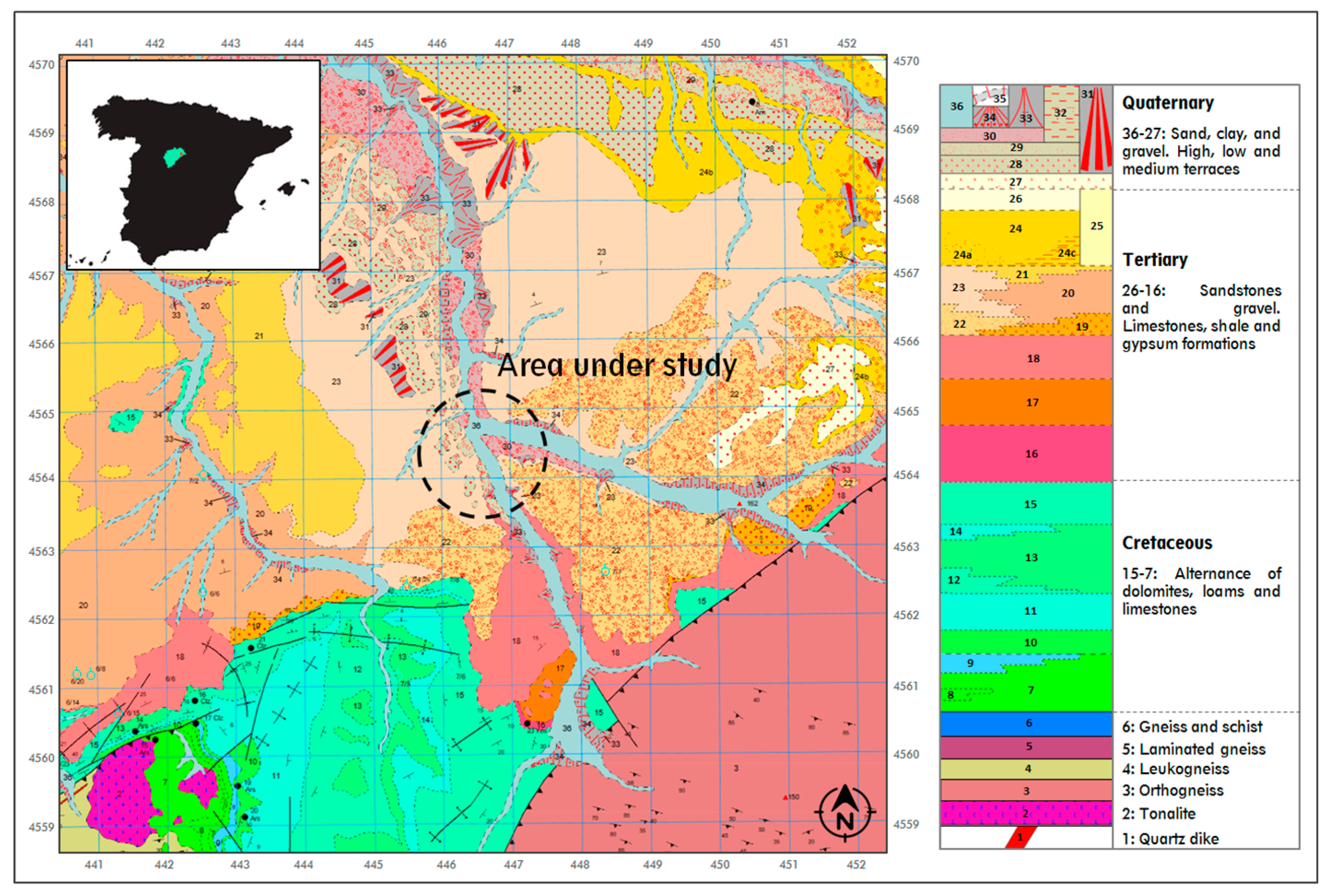
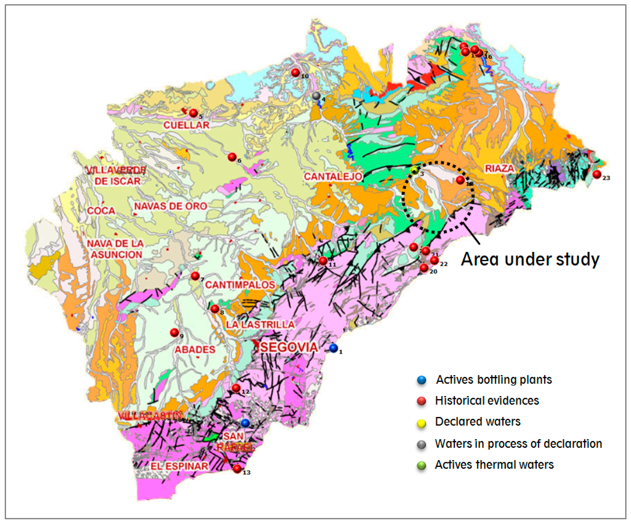
2.1. Characterization of the Area under Study
2.1.1. Tertiary
2.1.2. Calcareous Mesozoic
2.1.3. Paleozoic
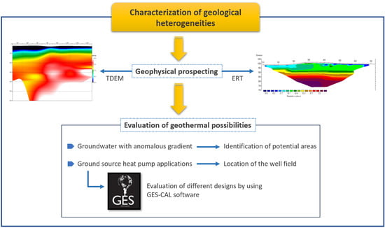
2.2. Geophysical Prospecting
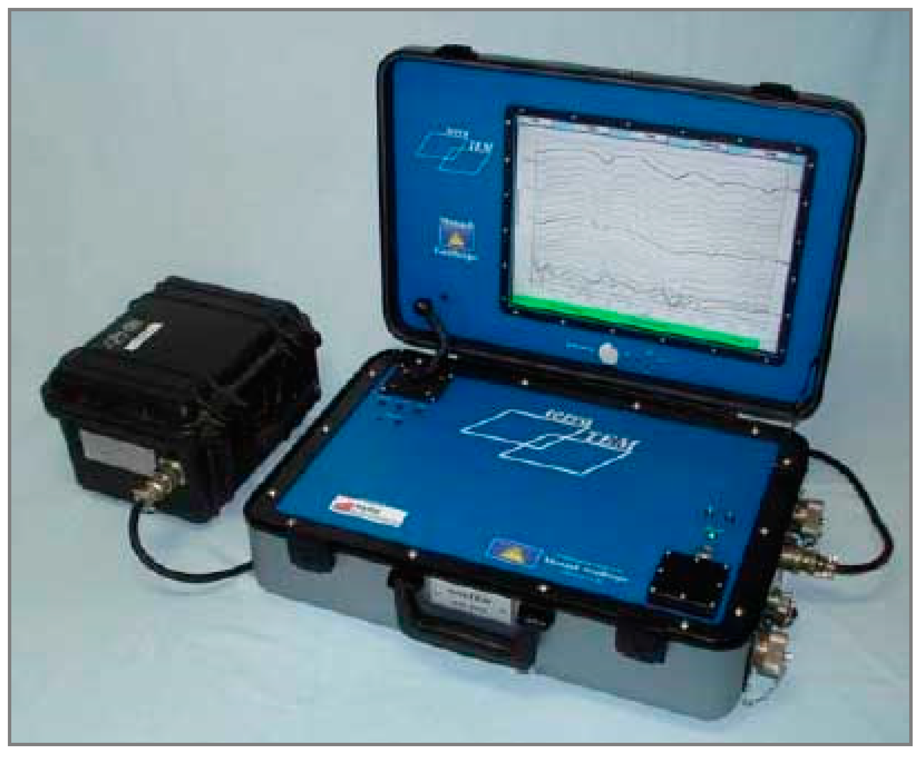
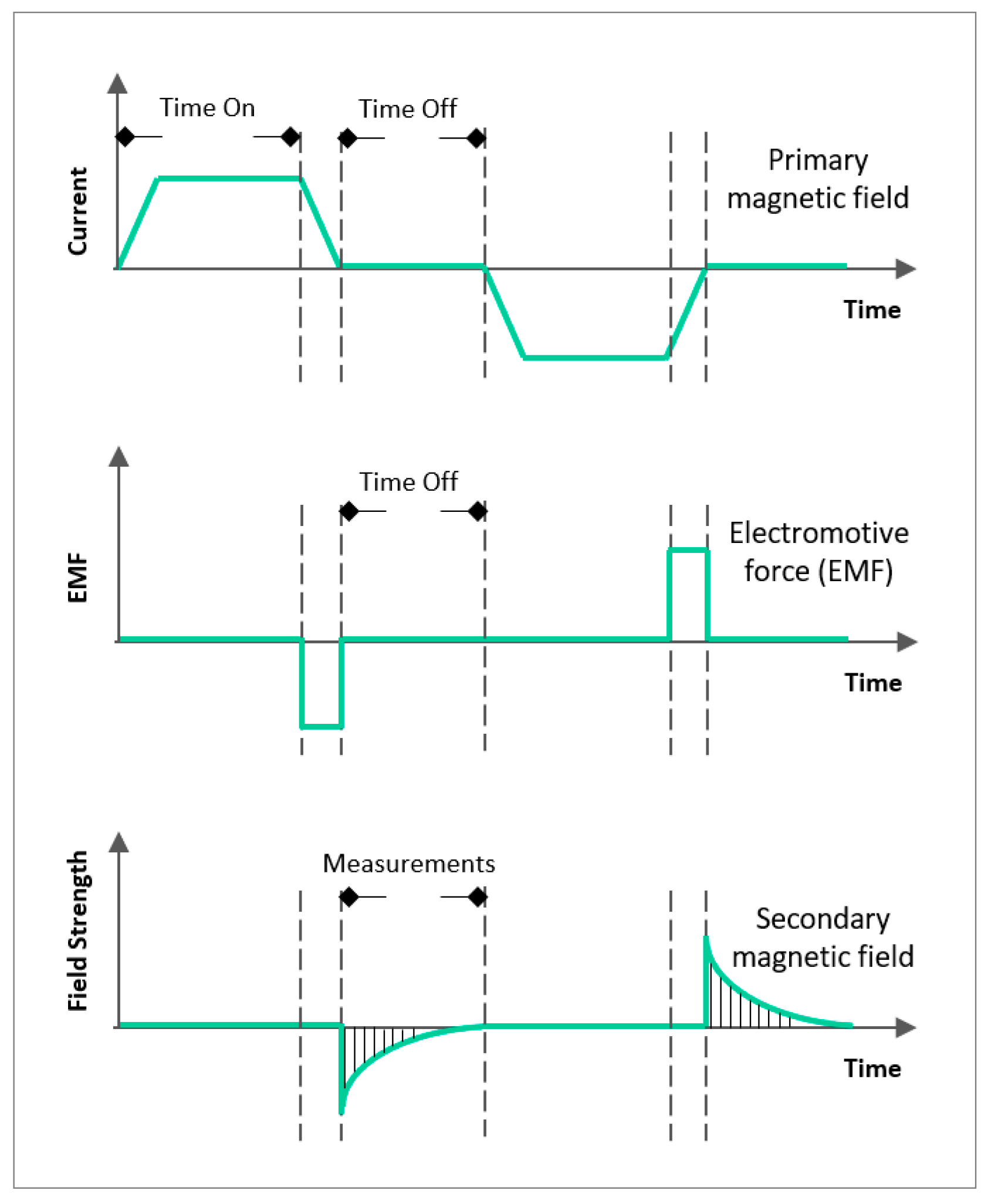
2.2.1. TDEM
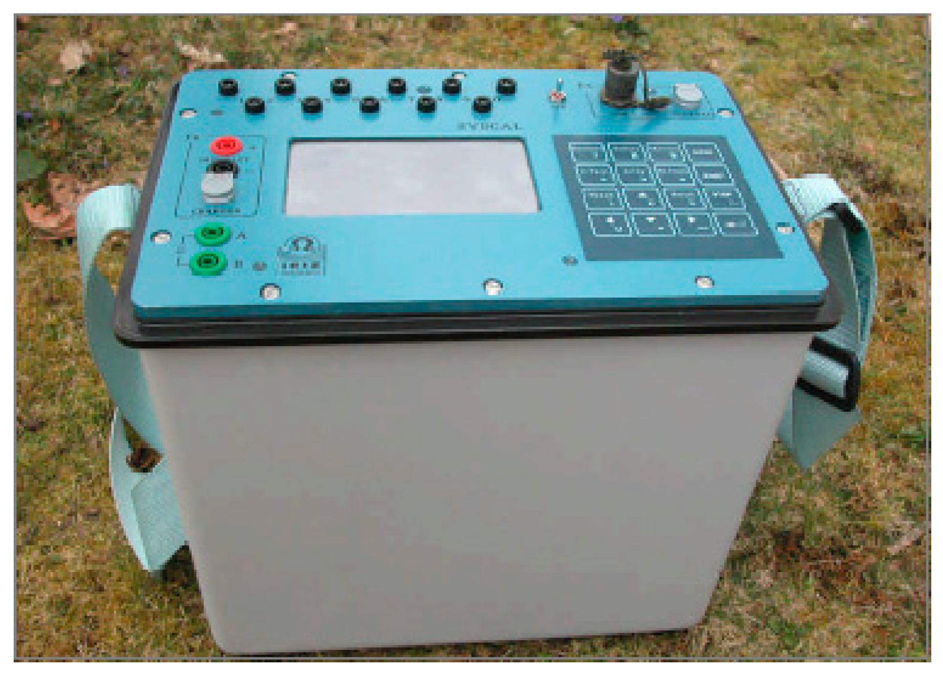
2.2.2. ERT
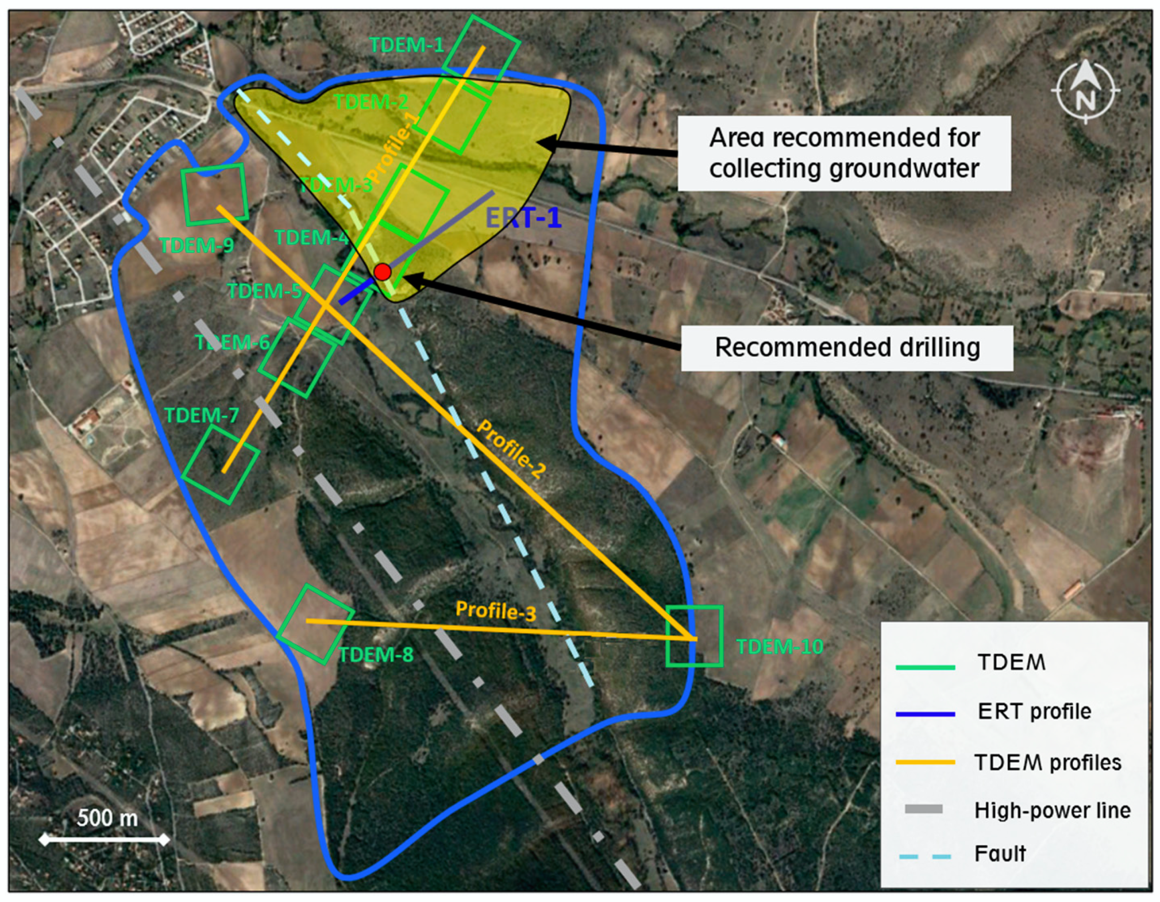
2.3. Field Work
3. Results
4. Discussion
4.1. Anomalous Geothermal Possibilities
4.2. Ground-Source Heat-Pump Uses
5. Conclusions
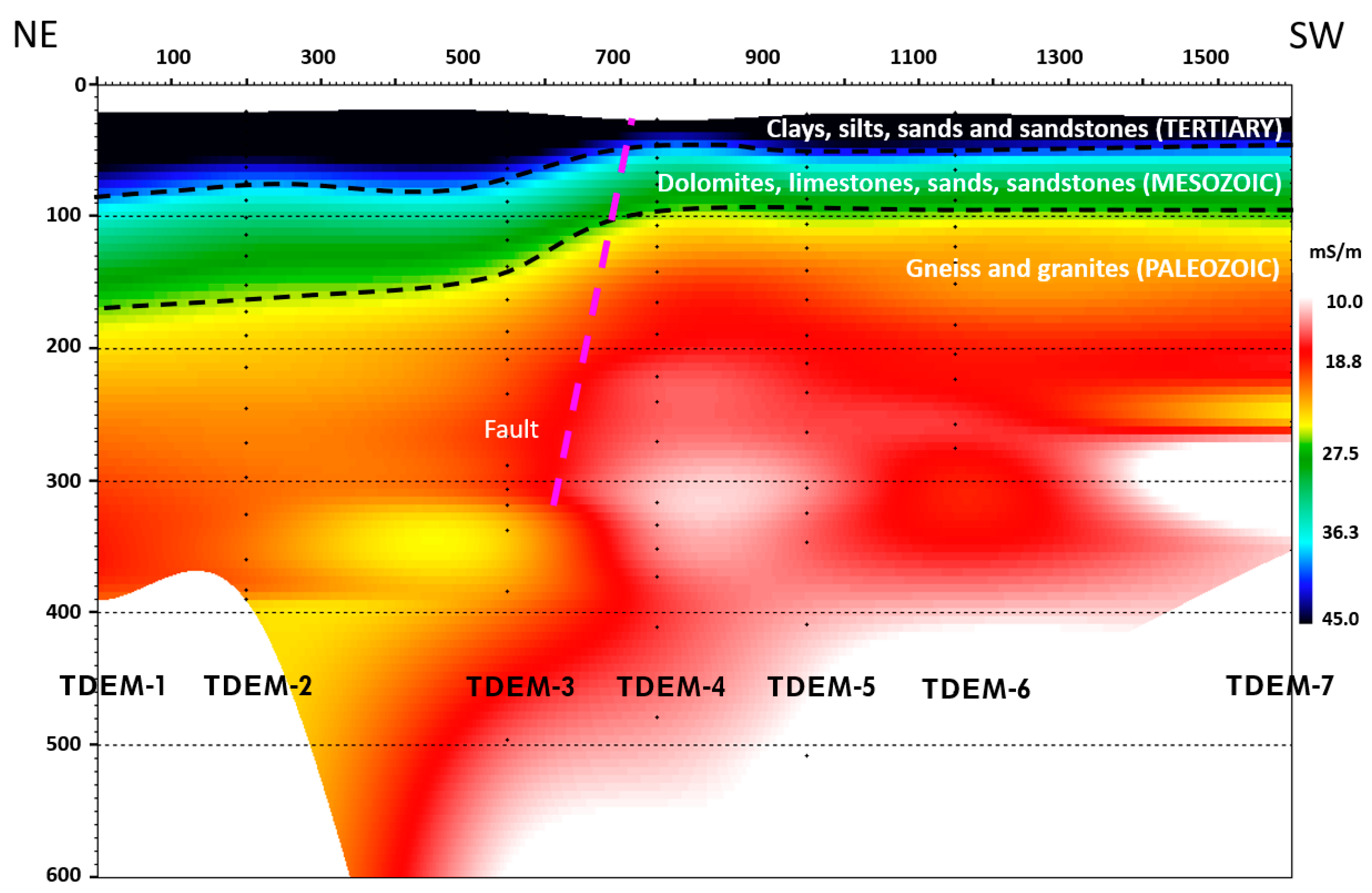
- The investigated area is located on the SE edge of the tertiary depression belonging to the Duero Basin. The most superficial geological unities are principally detrital materials: clays, sands, gravels, silts, and sandstones. More in depth, dolomites, limestones, and sandstones are found to finally reach the Paleozoic level (gneiss and granites). Results derived from the implementation of geophysics have allowed us to define the thickness of each layer of materials in the entire area under study.
- Regarding the exploitation of groundwater resources, the highest possibilities of locating thermal waters were detected in the NE side of the study area. More specifically, the fault associated to the Duratón River is considered the most favorable location to exploit the mentioned resource.
- In addition to the possible use of thermal waters, the implementation of ground-source heat-pump systems was analyzed in this research. Even though, in all the area under study, it is possible to install this kind of energy, the information obtained from the geophysical tests has also allowed us to define the most appropriate location of the geothermal well field. The GES-CAL tool was used to compare the design of the shallow geothermal system in different locations of the area. Through this analysis, it has verified that the precise location of the geothermal wells could mean significant economic savings, being also important to avoid possible technical problems during the drilling process.
Author Contributions
Funding
Acknowledgments
Conflicts of Interest
Appendix A
- TDEM equipment

| TerraTEM | |
|---|---|
| Transmitter Output | 10 Amps. (max.) |
| Receivers | 1 Channel |
| High-Resolution Sampling Rates | 500 kHz |
| Data Visualization and Processing in Field | Standard Software |
| Storage Device | 1 GB Flash Disk |
| GPS Receiverº | 12 Channels |
| Communications | USB and RS-232 Standard |
| Extra Stacking Options and Gain Functions | 10 Selectable Gain Settings from 1 to 8.000 |
| Operating Temperature | −10–40 °C |
| Resolution | 23 nV |
| Transmitter Current | 50 A at 6 V through to 120 V (6 kW) |
- ERT equipment
| Syscal Pro | |
|---|---|
| Transmitter max. voltage | 800 V |
| Transmitter max. current | 2.5 A, accuracy 0.2% |
| Transmitter max. power | 250 W |
| Receiver max. voltage | 15 V |
| Receiver resolution | 1 microV |
| Electrodes | Up to 4000 can be used |
| Data flash memory | More than 21,000 readings |
| Serial link | RS-232 data download |
| Power supply | Two internal rechargeable 12 V, 7.2 Ah Optional external 12 V batteries |
| Casing | Shock resistant fiber-glass case |
| Operating Temperature | −20–70 °C |
Appendix B

References
- Armstead, H.C. Geothermal Energy: Its Past, Present and Future Contribution to the Energy Needs of Man, 2nd ed.; E. & F.N Spon: New York, NY, USA; London, UK, 1983. [Google Scholar]
- Bodvarsson, G. Evaluation of geothermal prospects and the objectives of geo-thermal exploration. Geoexploration 1970, 8, 7–17. [Google Scholar] [CrossRef]
- Sena-Lozoya, E.B.; González-Escobar, M.; Gómez-Arias, E.; González-Fernández, A.; Gómez-Ávila, M. Seismic exploration survey northeast of the Tres Virgenes Geothermal Field, Baja California Sur, Mexico: A new Geothermal prospect. Geothermics 2020, 84, 101743. [Google Scholar] [CrossRef]
- Kearey, P.; Brooks, M.; Hill, I. An Introduction to Geophysical Exploration; John Wiley & Sons: Hoboken, NJ, USA, 2013. [Google Scholar]
- Aretouyap, Z.; Nouck, P.N.; Nouayou, R. A discussion of major geophysical methods used for geothermal exploration in Africa. Renew. Sustain. Energy Rev. 2016, 58, 775–781. [Google Scholar] [CrossRef]
- Mariita, N.O. Strengths and weaknesses of gravity and magnetics as exploration tools for geothermal energy. In Proceedings of the Short Course V on Exploration for Geothermal Resources, Naivasha, Kenya, 29 Octomber–19 November 2010. [Google Scholar]
- DomraKana, J.; Djongyang, N.; Raïdandi, D.; Nouck, P.N.; Dadjé, A. A review of geophysical methods for geothermal exploration. Renew. Sustain. Energy Rev. 2015, 44, 87–95. [Google Scholar] [CrossRef]
- Bibby, H.M.; Risk, G.F.; Caldwell, T.G.; Bennie, S.L. Misinterpretation of electrical resistivity data in geothermal prospecting: A case study from the Taupo Volcanic Zone. In Geological and Nuclear Sciences, Proceedings of the World Geothermal Congress; World Geothermal Congress: Antalya, Turkey, 2005; pp. 1–8. [Google Scholar]
- Deckert, H.; Bauer, W.; Abe, S.; Horowitz, F.G.; Schneider, U. Geophysical greenfield exploration in the permo-carboniferous Saar–Nahe basin—The Wiesbaden Geothermal Project, Germany. Geophys. Prospect. 2018, 66, 144–160. [Google Scholar] [CrossRef]
- Subasinghe, N.D.; Nimalsiri, T.B.; Suriyaarachchi, N.B.; Hobbs, B.; Fonseka, M.; Dissanayake, C. Study of Thermal Water Resources in Sri Lanka Using Time Domain Electromagnetics (TDEM). En Advanced Materials Research; Trans Tech Publications Ltd.: Freienbach, Switzerland, 2014; pp. 3198–3201. [Google Scholar]
- Fadillah, T.; Sulistijo, B.; Notosiswoyo, S.; Kristanto, A.; Yushantarti, A. The Resistivity Structure of Aluvial in Geothermal Prospect. Using Time Domain Electromagnetic Methode (TDEM) Survey. In Proceedings of the World Geothermal Congress 2015, Melbourne, Australia, 19–25 April 2015. [Google Scholar]
- Sáez Blázquez, C.; Martín, A.F.; García, P.C.; González-Aguilera, D. Thermal conductivity characterization of three geological formations by the implementation of geophysical methods. Geothermics 2018, 72, 101–111. [Google Scholar] [CrossRef]
- Martín Nieto, I.; Farfán Martín, A.; Sáez Blázquez, C.; González-Aguilera, D.; Carrasco García, P.; Farfán Vasco, E.; Carrasco García, J. Use of 3D electrical resistivity tomography to improve the design of low enthalpy geothermal systems. Geothermics 2019, 79, 1–13. [Google Scholar] [CrossRef]
- Bibby, H.M.; Dawson, G.B.; Rayner, H.H.; Bennie, S.L.; Bromley, C.J. Electrical resistivity and magnetic investigations of the geothermal systems in the Rotorua area, New Zealand. Geothermics 1992, 21, 43–64. [Google Scholar] [CrossRef]
- Tang, X.; Zhang, J.; Pang, Z.; Hu, S.; Tian, J.; Bao, S. The eastern Tibetan Plateau geothermal belt, western China: Geology, geophysics, genesis, and hydrothermal system. Tectonophysics 2017, 717, 433–448. [Google Scholar] [CrossRef]
- Abubakar, A.J.A.; Hashim, M.; Pour, A.B. Remote sensing satellite imagery for prospecting geothermal systems in an aseismic geologic setting: Yankari Park, Nigeria. Int. J. Appl. Earth Obs. Geoinf. 2019, 80, 157–172. [Google Scholar] [CrossRef]
- Arzate, J.; Corbo-Camargo, F.; Carrasco-Núñez, G.; Hernández, J.; Yutsis, V. The Los Humeros (Mexico) geothermal field model deduced from new geophysical and geological data. Geothermics 2018, 71, 200–211. [Google Scholar] [CrossRef]
- Long, C.L.; Kaufmann, H.E. Reconnaissance geophysics of a known geothermal resource area, Weiser, Idaho and Vale, Oregon. Geophysics 1980, 45, 312–322. [Google Scholar] [CrossRef]
- Volpi, G.; Manzella, A.; Fiordelisi, A. Investigation of geothermal structures by magnetotellurics (MT): An example from the Mt. Amiata area, Italy. Geothermics 2003, 32, 131–145. [Google Scholar] [CrossRef]
- Hermans, T.; Vandenbohede, A.; Lebbe, L.; Nguyen, A. shallow geothermal experiment in a sandy aquifer monitored using electric resistivity tomography. Geophysics 2012, 77, 11–21. [Google Scholar] [CrossRef] [Green Version]
- Magna 50. Mapa Geológico de España 1:50.000; Instituto Geológico y Minero de España: Sepúlveda, Spain, 2003; hoja 431. [Google Scholar]
- Aguas Minerales y Termales de España. IGME, Instituto Geológico y Minero de España. Available online: http://aguasmineralesytermales.igme.es/inicio.aspx (accessed on 1 January 2020).
- Hapsoro, C.A.; Srigutomo, W.; Purqon, A. 3-D Modeling of Layered Earth Structure in the Geothermal Systems Using Time Domain Electromagnetics (TDEM) Method. IOP Conference Series: Earth and Environmental Science; IOP Publishing: Bristol, UK, 2019; Volume 318. [Google Scholar]
- Goldman, M.; Rabinovich, B.; Rabinovich, M.; Gilad, D.; Gev, I.; Schirov, M. Application of the integrated NMR-TDEM method in groundwater exploration in Israel. J. Appl. Geophys. 1994, 31, 27–52. [Google Scholar] [CrossRef]
- Descloitres, M.; Chalikakis, K.; Legchenko, A.; Moussa, A.M.; Genthon, P.; Favreau, G.; Le Coz, M.; Boucher, M.; Oï, M. Investigation of groundwater resources in the Komadugu Yobe Valley (Lake Chad Basin, Niger) using MRS and TDEM methods. J. Afr. Earth Sci. 2013, 87, 71–85. [Google Scholar] [CrossRef]
- Fitterman, D.V.; Stewart, M.T. Transient Electromagnetic Sounding for Groundwater. Geophysics 1986, 51, 889–1033. [Google Scholar] [CrossRef]
- Kumar, D.; Thiagarajan, S.; Rai, S.N. Deciphering geothermal resources in Deccan Trap region using electrical resistivity tomography technique. J. Geol. Soc. India 2011, 78, 541–548. [Google Scholar] [CrossRef]
- Carrier, A.; Lupi, M.; Fishanger, F.; Nawratil de Bono, C. Deep-reaching electrical resistivity tomography (ERT) methods for middle-enthalpy geothermal prospection in the Geneva Basin, Switzerland. In Proceedings of the EGU General Assembly Conference Abstracts, Vienna, Austria, 8–13 April 2018; p. 20. [Google Scholar]
- Chabaane, A.; Redhaounia, B.; Gabtni, H. Combined application of vertical electrical sounding and 2D electrical resistivity imaging for geothermal groundwater characterization: Hammam Sayala hot spring case study (NW Tunisia). J. Afr. Earth Sci. 2017, 134, 292–298. [Google Scholar] [CrossRef]
- Maté-González, M.Á.; Sánchez-Aparicio, L.J.; Sáez Blázquez, C.; Carrasco García, P.; Álvarez-Alonso, D.; de Andrés-Herrero, M.; García-Davalillo, J.C.; González-Aguilera, D.; Herández Ruiz, M.; Jordá Bordehore, L.; et al. On the Combination of Remote Sensing and Geophysical Methods for the Digitalization of the San Lázaro Middle Paleolithic Rock Shelter (Segovia, Central Iberia, Spain). Remote Sens. 2019, 11, 2035. [Google Scholar] [CrossRef] [Green Version]
- Daniels, F.; Alberty, R.A. Physical Chemistry; Mir: Moscow, Russia, 1966; p. 291. [Google Scholar]
- Mainoo, P.A.; Manu, E.; Yidana, S.M.; Agyekum, W.A.; Stigter, T.; Duah, A.A.; Preko, K. Application of 2D-Electrical resistivity tomography in delineating groundwater potential zones: Case study from the voltaian super group of Ghana. J. Afr. Earth Sci. 2019, 160, 103618. [Google Scholar] [CrossRef]
- Zhou, B.; Moosoo, W. Multi-Parameter Tomographic Inversion for Imaging 2D Electrical Resistivity Anisotropy. 1st Conference on Geophysics for Geothermal-Energy Utilization and Renewable-Energy Storage. Eur. Assoc. Geosci. Eng. 2019, 1, 1–5. [Google Scholar]
- deGroot-Hedlin, C.; Constable, S. Occam’s inversion to generate smooth, two-dimensional models from magnetotelluric data. Geophysics 1990, 55, 1613–1624. [Google Scholar] [CrossRef]
- Rajesh, R.; Tiwari, R.K. FORTRAN code to convert resistivity Vertical Electrical Sounding data to RES2DINV format. Site Characterisation Using Multi-Channel Anal. Surf. Waves Var. Locat. Kumaon Himalayas India 2018, 22, 359–363. [Google Scholar]
- Istiqomah, A.N. Analisis Komparasi Inversi Software Res2Dinv dan Ipi2Win Pada Metode Vertical Electrical Sounding (VES); SKRIPSI Mahasiswa UM: Kuala Lumpur, Malaysia, 2019. [Google Scholar]
- Sáez Blázquez, C.; Martín Nieto, I.; Mora, R.; Farfán Martín, A.; González-Aguilera, D. GES-CAL: A new computer program for the design of closed-loop geothermal energy systems. Geothermics 2020, 87, 101852. [Google Scholar] [CrossRef]
- Structural solutions file. In Technical Building Code, CTE; Institute of Structural Sciences of Eduardo Torroja and Structural Institute of Castilla y León: Castilla y León, Spain, 2007.
- Agencia Estatal de Meteorología (AEMET). Series of Annual Average Temperatures of AEMET Stations (Spain). Observations of the Thirty-Year Period 1981–2010, Completed, Refined and Homogenized; Agencia Estatal de Meteorología (AEMET): Madrid, Spain, 2010.


| Classification | Description |
|---|---|
| 18-Historical evidence | 180 m deep spring water drilling Lithology: clays, sands, and gravels Water temperature: 14.7 °C |
| 3-Declared water | Natural spring Lithology: Cretaceous limestones Water temperature: 20.8 °C |
| 20-Historical evidence | Unavailable additional information |
| 21-Historical evidence | Natural spring Lithology: carbonated Cretaceous Water temperature: 11.7 °C |
| 22-Historical evidence | Unavailable additional information |
| 23-Historical evidence | Unavailable additional information |
| Test | X | Y |
|---|---|---|
| TDEM-1 | 447,377 | 4,564,903 |
| TDEM-2 | 447,289 | 4,564,603 |
| TDEM-3 | 447,165 | 4,564,251 |
| TDEM-4 | 446,949 | 4,564,139 |
| TDEM-5 | 446,641 | 4,563,959 |
| TDEM-6 | 446,353 | 4,563,763 |
| TDEM-7 | 446,277 | 4,563,283 |
| TDEM-8 | 446,637 | 4,562,667 |
| TDEM-9 | 446,257 | 4,564,295 |
| TDEM-10 | 448,085 | 4,562,743 |
| Profile 1 | X | Y |
|---|---|---|
| Starting point | 446,708 | 4,564,016 |
| Ending point | 447,334 | 4,564,353 |
| UTM Coordinates | X | Y |
|---|---|---|
| Recommended drilling | 446,872 | 4,564,070 |
| Cases | Ground Thermal Conductivity (W/mK) | Total Drilling Length * (m) | Initial Investment (€) |
|---|---|---|---|
| Case 1 | 2.178 | 136 | 22,993.38 |
| Case 2 | 1.920 | 152 | 25,019.23 |
| Case 3 | 1.286 | 218 | 29,729.28 |
© 2020 by the authors. Licensee MDPI, Basel, Switzerland. This article is an open access article distributed under the terms and conditions of the Creative Commons Attribution (CC BY) license (http://creativecommons.org/licenses/by/4.0/).
Share and Cite
Sáez Blázquez, C.; Carrasco García, P.; Nieto, I.M.; Maté-González, M.Á.; Martín, A.F.; González-Aguilera, D. Characterizing Geological Heterogeneities for Geothermal Purposes through Combined Geophysical Prospecting Methods. Remote Sens. 2020, 12, 1948. https://doi.org/10.3390/rs12121948
Sáez Blázquez C, Carrasco García P, Nieto IM, Maté-González MÁ, Martín AF, González-Aguilera D. Characterizing Geological Heterogeneities for Geothermal Purposes through Combined Geophysical Prospecting Methods. Remote Sensing. 2020; 12(12):1948. https://doi.org/10.3390/rs12121948
Chicago/Turabian StyleSáez Blázquez, Cristina, Pedro Carrasco García, Ignacio Martín Nieto, Miguel Ángel Maté-González, Arturo Farfán Martín, and Diego González-Aguilera. 2020. "Characterizing Geological Heterogeneities for Geothermal Purposes through Combined Geophysical Prospecting Methods" Remote Sensing 12, no. 12: 1948. https://doi.org/10.3390/rs12121948