Article

Assessment of the Extreme Precipitation by Satellite Estimates over South America

by
Rayana Santos Araujo Palharini
1,*,
Daniel Alejandro Vila
1,
Daniele Tôrres Rodrigues
2,
David Pareja Quispe
1,
Rodrigo Cassineli Palharini
3,
Ricardo Almeida de Siqueira
1 and
João Maria de Sousa Afonso
1
1
National Institute for Space Research (INPE), Av. dos Astronautas, 1758-Jardim da Granja, São José dos Campos-SP 12227-010, Brazil
2
Departament of Statistics, Federal University of Piauí (UFPI), Av. Universitária, Ininga, Teresina-PI 64049-550, Brazil
3
Department of Mechanical Engineering, Universidad Técnica Federico Santa María, Vicuña Mackenna 3939, San Joaquín, Santiago 8940000, Chile
*
Author to whom correspondence should be addressed.
Remote Sens. 2020, 12(13), 2085; https://doi.org/10.3390/rs12132085
Submission received: 20 April 2020 / Revised: 2 June 2020 / Accepted: 14 June 2020 / Published: 29 June 2020

Abstract

:
In developing countries, accurate rainfall estimation with adequate spatial distribution is limited due to sparse rain gauge networks. One way to solve this problem is the use of satellite-based precipitation products. These satellite products have significant spatial coverage of rainfall estimates and it is of fundamental importance to investigate their performance across space–time scales and the factors that affect their uncertainties. In the open literature, some studies have already analyzed the ability of satellite-based rain estimation products to estimate average rainfall values. These investigations have found very close agreement between the estimates and observed data. However, further evaluation of the satellite precipitation products is necessary to improve their reliability to estimate extreme values. In this scenario, the main goal of this work is to evaluate the ability of satellite-based precipitation products to capture the characteristics of extreme precipitation over the tropical region of South America. The products evaluated in this investigation were 3B42 RT v7.0, 3B42 RT v7.0 uncalibrated, CMORPH V1.0 RAW, CMORPH V1.0 CRT, GSMAP-NRT-no gauge v6.0, GSMAP-NRT- gauge v6.0, CHIRP V2.0, CHIRPS V2.0, PERSIANN CDR v1 r1, CoSch and TAPEER v1.5 from Frequent Rainfall Observations on GridS (FROGS) database. Some products considered in this investigation are adjusted with rain gauge values and others only with satellite information. In this study, these two sets of products were considered. In addition, gauge-based daily precipitation data, provided by Brazil’s National Institute for Space Research, were used as reference in the analyses. In order to compare gauge-based daily precipitation and satellite-based data for extreme values, statistical techniques were used to evaluate the performance the selected satellite products over the tropical region of South America. According to the results, the threshold for rain to be considered an extreme event in South America presented high variability, ranging from 20 to 150 mm/day, depending on the region and the percentile threshold chosen for analysis. In addition, the results showed that the ability of the satellite estimates to retrieve rainfall extremes depends on the geographical location and large-scale rainfall regimes.

Graphical Abstract

1. Introduction

Precipitation is one of the most important meteorological variables to investigate in the hydrological cycle context. When precipitation occurs in a very intense or extreme way, it can cause significant social, economic and environmental impacts. The meteorological systems responsible for intense rainfall are complex and evolve rapidly, making measurement difficult. In addition, due to the morphology of these systems, rainfall can occur in one place and not in others, which makes precipitation measurements in certain regions a real challenge [1].
In recent decades, the interest in investigating the impact of extreme events has been growing due their effects on daily life [2,3,4]. In this scenario, different techniques have been developed to monitor precipitation using satellites. However, extreme precipitation data collected by the satellites are difficult to process, requiring complex algorithms for this task [5]. Improvement of these algorithms for data retrieval is essential to quantify extreme events in terms of frequency and intensity, and to generate useful information for decision-makers.
The use of satellite-based retrievals is promising, and their use has increased since the launch of missions such as the Tropical Rainfall Measuring Mission (TRMM) [6] and the Global Precipitation Measurement (GPM) mission [7]. These initiatives provide quasi-global coverage and better quantitative description of rain processes. Although the quality of satellite rainfall products has improved in recent years, their algorithms require validation studies through comparisons with observational data and physical process approaches.
Some studies have observed that satellite-based retrievals for extreme precipitation events, usually caused by convective systems, fall short of expectations [5] and that South America experiences some of the most intense mesoscale convective systems (MCSs) on Earth [8].
In general, satellite observations tend to underestimate the rainfall when convective systems are shallow and overestimate them when convective systems are deep [9]. Furthermore, the presence of complex topography in South America, like the Andes mountain range with its snow-covered surfaces and heavy precipitation from warm clouds in areas such as northeastern Brazil and the Amazon, makes satellite estimation a very difficult task [10,11,12,13]. It is a particular challenge to estimate warm rain, and most studies of precipitation estimation with satellite data over land focus in rain-ice processes, making it hard to detect warm rain by the algorithms [14,15]. In Brazil, for example, about 80% of the clouds over the coastal areas of the Northeast region and adjacent ocean are classified as shallow convective, responsible for generating extreme warm rain events [12]. Rodrigues et al. [16] showed that the quality of extreme satellite estimates in northeastern Brazil depends on the season, location, and time scale in which the precipitation events occur. Their study indicated that accumulated rain in two days showed better results for the quality of the extreme precipitation estimates coming from the satellite. However, those results cannot be extrapolated to other regions and rainfall regimes, as shown by other researchers who have performed global analysis [5,17].
Several limitations of data sampling (due to the intermittent time-space behavior of precipitation), sensor design (due to spatial, temporal and spectral resolution) and algorithm design are also sources of uncertainties for extreme satellite-based retrievals. At the same time, the use of satellite-based datasets is fundamental to provide global coverage and a better quantitative description of rain processes. In this respect, the quality of satellite rainfall products has improved in recent decades. Satellite rainfall products (SRPs hereafter) have been improved in terms of temporal and spatial resolution. However, their performance needs to be understood across space–time scales and other uncertainty factors should be identified. Some studies have already evaluated the ability of satellite-based rain estimation products to estimate average rainfall values. These investigations have revealed very close estimates to observed data, such as [18,19,20,21]. These have analyzed different satellite-based rainfall estimation for Africa, Austria and China, by evaluating the average behavior of rain intensity over the respective time series chosen by the authors. But further investigation is needed of the ability of these satellite-based products to estimate extreme rainfall values.
In this context, the main goal of this study is to assess the ability of satellite-based precipitation products to capture the characteristics of extreme precipitation over the tropical region of South America using different satellite precipitation estimation products from a new dataset called Frequent Rainfall Observations on GridS (FROGS) [22], and to compare them with the rain gauge dataset from the National Institute for Space Research (INPE) for the period 2012–2016. To compare SRPs and rain-gauge data, maximum values and 99th percentiles of time series were used to identify extreme events. Statistical metrics such as bias, correlation and mean square error were used.

2. Materials and Methods
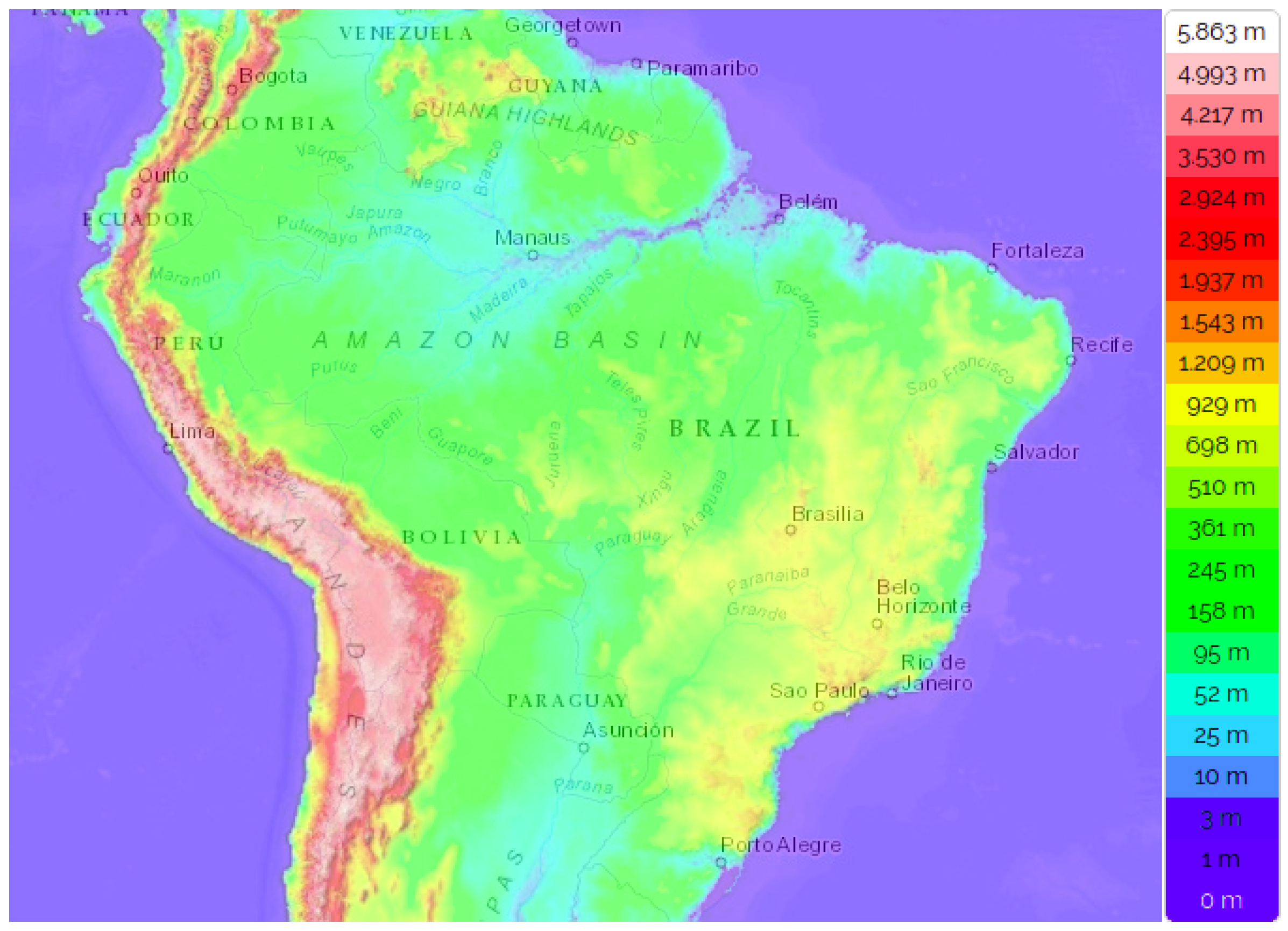
2.1. Study Area

South America has an area of about 17.8 million km 2 , contains 6% of the world’s population, and is divided into 12 countries. The precipitation in South America is influenced by a large number of meteorological systems, which in turn can be influenced by the topographic characteristics in the region, as shown in Figure 1. A review of the atmospheric systems and a schematic representation of all the systems that occur in the low and high troposphere over South America is available in [23].
The domain analyzed in this investigation is contained in the coordinates from 30 S to 15 N and from 90 W to 30 W, corresponding to the tropical region of South America. We considered a period of five years, ranging from 2012 to 2016.

2.2. Data

2.2.1. Rainfall Satellite-Based Products

The Frequent Rainfall Observations on GridS (FROGS) dataset (DOI:10.14768/06337394-73A9- 407C-9997-0E380DAC5598), which is composed of daily precipitation gridded products that include satellites, ground-based and reanalysis products adjusted to a common 1 × 1 grid resolution, were used in this study. The dataset was downloaded from the ESPRI/IPSL repository.
Developed by [22], the FROGS database was built to put all products from different groups such as NASA, NOAA, JAXA among others, in a common resolution. Each product was originally formulated with different purposes, considering different areas and different time scales and resolutions. Some products contain global information, others quasi-global and still others specific regions. Also, there are products that consider only the ocean or land areas, and others that consider both. For this reason, the FROGS dataset was built to offer accessible data on daily precipitation products with a common grid of 1 × 1 , to provide support to clarify some uncertainties that are inherent in all precipitation products by making them comparable. The FROGS database is formed by 32 products, where the files are produced in NETCDF-4 format and contain information such as longitude, latitude, time and rain intensity. To perform this investigation, we considered the subset of SRPs for the period ranging from 2012 to 2016.
The SRPs selected in this study are described below.
The 3B42RT is a near-real-time product, also known as the TRMM multi-satellite Precipitation Analysis (TMPA) algorithm - Real-Time [24], where passive microwave (PMW) and infrared (IR) data are combined and the historical rain gauge information is incorporated in the calibrated product;
The Global Satellite Mapping of Precipitation (GSMAP) product [25] is based on microwave estimation of rainfall but also use IR geostationary imagery to extrapolate the PMW estimates. Rain gauge observations are used to correct for bias;
The Climate Prediction Center morphing technique (CMORPH) [26] is a product that combines PMW and IR data to ’morph’ the PWM estimated fields. A bias correction technique, using Climate Prediction Center (CPC) rain gauge analysis [27], is applied over land surfaces for the V1.0 CRT version;
The Combined Scheme approach (CoSch) [28] is a product that uses the Real-Time—TRMM Multi-satellite Precipitation Analysis (TMPA) algorithm and rain gauge data from the Global Telecommunications System (GTS) and multiple institutions in Latin America to remove the bias from TMPA;
The Tropical Amount of Precipitation with an Estimation of ERror (TAPEER) is a product based on the GOES precipitation index technique [29], which merges geostationary infrared images with microwave instantaneous rain rate estimates;
The Climate Hazards Infrared Precipitation (CHIRP) [30] is a product based on infrared observations from geostationary observations in a GOES. The CHIRPS product is a merger of rain station information with CHIRP estimates using a weighted average of the closest stations;
The Precipitation Estimation from Remotely Sensed Information using Artificial Neural Networks—Climate Data Record (PERSIANN-CDR) [31] is an infrared-based product that uses neural networks to obtain rain rate information.
The short names and version of products used are: 3B42 RT v7.0, 3B42 RT v7.0 uncalibrated, CMORPH V1.0 RAW, CMORPH V1.0 CRT, GSMAP-NRT-no gauge v6.0, GSMAP-NRT- gauge v6.0, CHIRP V2.0, CHIRPS V2.0, PERSIANN CDR v1 r1, CoSch and TAPEER v1.5. From here on they will be called, respectively, 3B42g, 3B42, CMORPH, CMORPHg, GSMAP, GSMAPg, CHIRP, CHIRPSg, PERSIANNg, COSCHg and TAPEER, where sub-index ‘g’ represents the versions with gauge correction. More information about the products can be found in [22] Table 1 below reports some characteristics of the satellite products used.

2.2.2. Rainfall Ground-Based Data

In this study, two different ground-based databases were analyzed. The first database came from Global Precipitation Climatology Center (GPCC), which is included in the FROGS product. This product is available in a grid with a resolution of 1 × 1 , considers rainfall information from around the globe from the Global Precipitation Climatology Center (GPCC), and uses a modified SPHEREMAP interpolation scheme [32]. The second database was provided by Brazil’s National Center for Space Research (INPE) and contains data from automatic and conventional rain gauges/stations from different networks in South America. This database is in DAT format and has been interpolated for regular 1 × 1 grids using the simple average and then converted to NETCDF format, ensuring the consistency of spatial and temporal resolutions for comparisons.
In order to consider only the grid points representative of the entire time series period, only 10% of the missing data was allowed for each grid point. Figure 2a,c show the percentage of the number of days where at least one gauge was reported for that grid point in the GPCC and INPE databases, respectively, and Figure 2b,d identify the grid points with a frequency larger than 90% from Figure 2a,c. In the latter case, the GPCC and INPE databases have 220 and 345 valid grid points respectively.
Grid points with more than 90% of days with gauge information (rain ≥ 0.0) were used. In this analysis, 220 grid points were accounted for from the GPCC FROGS database and 345 grid points from the INPE database. Analysis of the rain gauge data sets for GCCP and INPE revealed that the INPE database had greater spatial coverage. Comparison between the two datasets (not shown here) indicated a small difference between them. For this reason, we decided to choose the dataset provided by INPE to perform this work. So, the INPE rainfall database will be used hereafter as the reference for validation of satellite precipitation estimates for different products. It is important to mention there is no complete coverage of rain gauges in the study area in both databases considered. However, the INPE database covered a more complete data network with more grid points represented by rain gauges.
To ensure data quality, INPE performs an automatic data quality control that considers four steps: (i) range test, which seeks to eliminate gross errors outside the confidence interval; (ii) step test, which considers a maximum difference between consecutive values; (iii) internal consistency test, which makes an association between different meteorological parameters; and (iv) persistence test, which identifies the variability of measurements over a long period of time [33].

2.3. Methodology

2.3.1. Assessment of Satellites Products: Statistical Analysis

Statistical analysis was performed to compare satellite data with the gauge-based rainfall data. The objective of this comparison was to evaluate the ability of different algorithms to estimate extreme rainfall. In doing so, we considered the following statistical measures [34,35,36,37]:
(a) The correlation coefficient (r) refers to the agreement between satellite-based rainfall and gauge-based rainfall. The correlation coefficient ranges between 1 and + 1 . The value of + 1 indicates a perfect positive fit, in other words, a perfect linear correlation. We use the term positive correlation when r > 0, in which case as P G i grows, P S i also increases, and negative correlation when r < 0, and in this case as P G i grows, P S i decreases on average.
Where:
  • P G i is the gauge-based value at pixel i
  • P S i is the satellite-based precipitation value at pixel i
  • n is the number pixels included in the analysis.
    r = i = 1 n ( P S i P S m e a n ) ( P G i P G m e a n ) i = 1 n ( P S i P S m e a n ) 2 i = 1 n ( P G i P G m e a n ) 2
(b) RMSE: Root Mean Square Error is one of the most commonly used methods to measure the absolute average error and is sensitive to larger errors.
R M S E = 1 n i = 1 n ( P S i P G i ) 2
(c) BIAS indicates the average tendency of the satellite-based rainfall fields to be larger or smaller than the rain gauges; the best value is 0; negative (positive) values indicate an underestimation (overestimation).
B I A S = 1 n i = 1 n P S i P G i
(d) Standard Deviation is a measure of the amount of variation or dispersion of a set of values. A low standard deviation indicates that the values tend to be close to the mean of the set, while a high standard deviation indicates that the values are spread out over a wider range.
S T D = 1 n ( P S i P S m e a n ) 2
Taylor diagrams were used to facilitate comparison between the data estimated by different models and the reference data [38,39,40]. These diagrams are used to quantify the degree of correspondence between the modeled and observed data in terms of three statistics: Pearson correlation coefficient (r), root mean square error (RMSE), and standard deviation (std). The x and y axes represent the standard deviation of the estimated and observed data, respectively. The green arc represents the RMSE and the arc on the right side denotes positive Pearson correlation coefficient values. The colored circles inside the diagram represent the models (satellite products) and the white circle, over the x-axis, represents the reference data (INPE). The closer a model is to the observation point, the better the satellite product is. To compare the statistical behavior of the extreme precipitation values of the different satellite products, the graphs of the probability density function (PDF) and empirical cumulative distribution function (ECDF) of the maximum rainfall values and several percentile values were generated. To estimate the density curves, the non-parametric kernel method was used [41,42].
Denoted by f x (x), the PDF describes the behavior, in polygonal form, of the frequency distribution of a random variable. In this study, maximum rainfall and extreme rainfall threshold are represented by X. The probability (Prob) of the random variable being less than a given value of interest is calculated using the CDF (Fx(x)), represented by Equation (5):
F x ( x ) = P r o b ( X x ) = o o x f x ( x ) d x
Inversely, the corresponding PDF can be obtained by differentiating Equation below:
f x ( x ) = d F x ( x ) d x
The CDF of a continuous random variable is a non-decreasing function, and the validated expressions are: F x (−oo) = 0 and F x (+oo) = 1 [43,44,45,46].
In addition to the statistical measures and graphical analysis of PDF and ECDF, a statistical test was also used. A preliminary analysis was carried out to choose between a parametric test, where the assumptions of normality, independence and constant variance must be satisfied, and a non-parametric test, where these assumptions do not all hold. The databases used were independent, but did not satisfy the other assumptions, so the Wilcoxon-Mann-Whitney test was chosen [47]. This is a non-parametric test employed as an alternative to the Student t-test (parametric cases) for two independent samples [48,49,50]. The objective is to test whether two distributions are equal in location, that is, whether the data distribution (observed and estimated) has the same median, where in this case the medians of the extreme values were evaluated. To apply the Wilcoxon-Mann-Whitney test, it is assumed that F and G are the distribution functions corresponding to the observed and estimated data, and the null hypothesis states that the distributions are equal, H 0 : F(X) = G(Y). The test statistic is calculated by the equation below, ([47]):
U = m n + m ( m + 1 ) 2 S m
where m and n represent the number of elements in samples X and Y respectively; and S m denotes the sum of the ranks related to the sample elements X. To decide whether or not to reject the null hypothesis, the p-value (probability of obtaining a test statistic equal to or greater than the value observed in a sample) is calculated. When this is below the desired significance level (here 5%), the null hypothesis is rejected.

2.3.2. Characterization of Extreme Rainfall

Extreme rainfall is one of the most severe weather hazards affecting the globe. To investigate these extreme events, statistical tools can be used to interpret a dataset and to find a constant threshold. This threshold is based on the empirical distribution of the variable at each location so as to ensure that a given fraction of events will by definition be extreme.
The most common way to choose a threshold is to use the quantiles as cutoff points that divide the range of a probability distribution into contiguous intervals with equal probabilities. But there is still no consensus in meteorology about the precipitation thresholds for the identification of extreme events, so this is highly variable. Liebmann et al. [51] studied the interannual variability of the events of daily extreme precipitation in the state of São Paulo and defined as extreme events those in which the daily precipitation exceeds a percentage of its seasonal or annual average. In turn, [52] defined the criterion of a 50 mm/day isohyetal line enclosing an area of not less than 10,000 km 2 in the domain of southern Brazil. Dereczynski et al. [53] studied intense rainfall events in Rio de Janeiro during 1997 to 2006 and applied the percentile technique for each rain station. They observed a threshold higher than 30 mm for the daily precipitation totals corresponding to the 99th percentile of all rain stations considered. Alves et al. [54] investigated the main atmospheric characteristics associated with extreme precipitation events in northeastern Brazil and defined extreme events as daily accumulation of precipitation with values greater than or equal to 50 mm.
In this work, we applied the quantile technique by establishing values above a certain threshold. Using the empirical cumulative distribution function (ECDF), we carried out a preliminary study with the thresholds of 99.0, 99.5 and 99.9 percentiles and the maximum value of the distribution of precipitation over tropical South America during the five-year period.
In this study, the thresholds of 99.0 percentile (p99th, hereafter) and maximum value were chosen to characterize extreme precipitation events over South America. As shown in Figure 3a,d, there was a slight difference between the two approaches. While almost all algorithms underestimated the maximum value and there were large discrepancies among them, the p99th, even though considered to be an extreme value from a statistical point of view, showed better agreement among the algorithms when compared with the reference data. The first situation could be because the maximum values are highly sensitive to unfiltered outliers or very rare events in the probability distribution of the reference data and/or the FROGS dataset. The maximum and p99th are explored in Section 3.

3. Results And Discussion

Since the launch of the first satellite completely focused on precipitation studies (TRMM), the academic community has been evaluating the performance of satellite precipitation estimates obtained by different algorithms [24,55,56,57,58]. For a long time, these efforts were focused on obtaining the average rainfall characteristics on a global basis. It was found that, for average values, the estimates showed a pattern similar to the observed rainfall [59]. However, this does not happen with extreme rainfall values, where satellite estimates tend to underestimate or overestimate retrievals depending on the physical characteristics of rainfall systems (deep vs. shallow convection systems) and other regional factors like orography and local circulation patterns, among others [11].
To summarize the inter-product differences, zonal mean precipitation was performed (Figure 4) to aggregate the multiple measurements at each latitude band (2 bins) by plotting the mean rainfall. Note that for the average values, the estimates are close to the reference values (in black), presenting larger dispersion in equatorial latitudes (5 S to 10 N) and close to the southern edge of the region between 25 S to 30 S. According to the climatology, these two regions presented the largest rain accumulation in the studied region [60]. However, this disagreement among different algorithms and the reference data could be also due to a data sampling issue. While the central region has the largest amount of valid grid points per latitude band (see Figure 2d), the equatorial region has the smallest number of valid grid points. The southern region is in an average situation regarding the number of valid points (Figure 4).
While there is a reasonable agreement for the mean values, large differences are observed in the ECDF of the extreme values, as can be noted in Figure 3. Therefore, approaches to extreme precipitation analysis are described in the next two subsections: (i) maximum daily values, and (ii) p99th obtained for each database and the reference.

3.1. Extreme Rain from Maximum Daily Values

The same zonal mean analysis was performed for the maximum estimated values for each product and for the reference data, as shown in Figure 5. All products tended to underestimate the maximum precipitation values for almost all latitude bands, and larger dispersion was noticed for the same regions, as described for the mean values in Figure 4.
In equatorial latitudes (5 S to 10 N), there was an abrupt variation in the maximum values of rain, as can be seen in the reference data (black line), with variation from 60 mm to 120 mm in just a few degrees of latitude. This variation may be associated with the short-lived convective systems that are common in this region [61]. Also, the algorithms were unable to simulate the same behavior. In the region that comprises latitudes between 5 S to 20 S, there was minor variation of the maximum rainfall values, which were all near 100 mm. All algorithms underestimated the maximum rainfall in this central region of South America, but the dispersion among them was small. Latitudes between 20 S to 30 S had the highest values for maximum rainfall and tended to underestimate these values, while others were overestimated. This behavior will be analyzed later in this section.
Figure 6 shows the frequency of maximum rainfall using the probability distribution function (PDF) of satellite products in South America. According to this plot, the most frequent values were between approximately 75 mm/day and 100 mm/day for the studied region. As shown in the previous analysis, satellite estimates tended to underestimate, with several degrees of disagreement, the maximum values of the PDF.
According to the results, the distributions of the products 3B42, GSMAP, GSMAPg, CMORPHg, COSCHg presented the closest agreement with reference database’s PDF, as shown in Figure 6. However, according to the Wilcoxon-Mann-Whitney test, the distributions of the maximum precipitation values estimated by the GSMAP and 3B42g products were statistically equivalent to the distribution of the maximum precipitation values observed according to the reference database (p-value > 0.05). The data distributions estimated by the 3B42g and GSMAP products had medians of 84.11 mm and 77.27 mm, respectively. The reference dataset (INPE) was closest to the median of the data distribution (89.20 mm). On average, the products with the smallest biases were 3B42g, GSMAP and TAPEER, with −3.05 mm, −3.82 mm, and −7.79 mm respectively.
As mentioned, the Taylor diagram provides a concise statistical summary of how well patterns match each other in terms of their correlation, root mean-square error and standard deviation. In this case, the shortest Euclidean distance to the reference data represents the closest agreement. COSCHg presented the best agreement when compared with other algorithms, as shown in Figure 7. According to the plot, COSCHg presented the best metrics compared with other products, with the highest correlation coefficient (r = 0.72) and the smallest standard deviation and root mean square error (std = 26.9 and RMSE = 24.5).
COSCHg presented the closest metrics when compared with the reference data, with correlation coefficient (r) = 0.72, standard deviation (std) = 26.9, and root mean square error (RMSE) = 24.5 for the entire region. These results were expected based on [28], since the COSCHg product merges satellite estimates with daily gauge data. In this case, TMPA is used as a high-quality rainfall algorithm and a very similar database (that used as a reference), composed of daily rain gauge observations, is used to correct the bias of near real-time over South America. As shown in Figure 7, bias was negative for South America, indicating that all products tended to underestimate maximum rainfall values.
Figure 5 shows the distribution of extreme rainfall differences with latitude and behaviors for each product. In Figure 8, the spatial distribution of maximum rainfall (mm/day) occurred in each valid pixel during the period analyzed for all SRPs and the reference data. The maximum spatial pattern values showed a clear delimitation of maximum values for almost all SRPs. In the reference dataset (Figure 8M), the largest maximum rainfall values were achieved in the southern and northern regions of Brazil, while the smallest values were observed in the semiarid region of northeastern Brazil. This pattern was also observed, with different degrees of agreement, in all studied algorithms.
The behavior mentioned above may be associated with the different types of meteorological systems that occur in each region [23] as well as the composition of hydrometeors within the clouds. In the southern region, clouds with significant ice content and deep convection, characteristics are typically observed [15], while at the northeastern region clouds generally have shallow convection with little or no ice content [12].
Still referring to Figure 8, it shows differences between the estimated maximum values and the observed maximum values. All products tended to underestimate extreme rainfall values. However, products such as CHIRP (Figure 8A) and PERSIANN (Figure 8J) tended to underestimate these values in all regions. This could be due to the fact that both rely on infrared information for rainfall retrieval. Salio et al. [11] showed that other IR-based algorithms (Hydro Estimator in that case) have difficulty in retrieving the largest precipitation values.
The products without rainfall adjustments tended to underestimate the lowest values and overestimate the highest values, as it can be seen in the southern and the northeast regions of Brazil respectively, and as demonstrated in Figure 8A–D and Figure 8L). The results are similar to the results found by [62] for East Africa. According to the authors, the performance of satellite products is weaker when rainfall intensity is high, and after adjustments, they observed a closer estimate in some regions.
Figure 9 depicts the difference between the maximum rain in the reference data and the maximum rain estimated by each product at each grid point. Some products overestimated the maximum values in some regions (reddish colors) while underestimating them in others (bluish colors).
While some products (CHIRPS, CHIRP and PERSIANN, among others) underestimated the maximum value for almost the whole region, others had different behavior according to the region. GSMAP, 3B42g and TAPEER tended to overestimate the maximum values over the southern region while underestimating them in the central region. The regional analysis will be investigated in the near future to establish a relationship between anomalies of large and regional circulation patterns and extreme values.

3.2. Extreme Rain from 99th Percentile Threshold

The second approach used to analyze extreme precipitation over South America was application of the 99th percentile threshold. The zonal analysis was performed for the p99th values of each precipitation estimation product and reference data (in black), as shown in Figure 10. According to this plot, most of the products tended to underestimate p99th and the pattern is very similar to the maximum values with larger dispersion in the southern region between 30 S-25 S and close to the equator.
Figure 5 and Figure 10 indicate that both maximum and p99th values for products such as GSMAP, CMORPH, 3B42 and TAPEER overestimated the reference values between 30 S-20 S. These results are similar to those obtained by [5], who used other reference data sources (GPCC v2018 and CPC v1.0), considered all points on ocean/land and interpolated points. In the central region, underestimation is present in all products, with a smaller dispersion due to the larger number of valid points considered, while the equatorial region is noisier and has larger dispersion due to the smaller number of valid point considered in the comparison and the complex behavior of the rainfall systems over the Amazonian region.
A similar analysis was performed for the maximum values, as shown in Figure 11. This plot depicts the frequency of the 99th percentile for rainfall using the probability distribution function (PDF) of satellite products from South America. According to the reference data, the most frequent p99th daily values were between 30 mm/day and 50 mm/day. This analysis considered daily rainfall values ≥ 0.0 mm in order to analyze the p99th for each grid point, and the same amount of data was present in each distribution.
Still referring to Figure 11, according to the PRF’s PDF, each product had a different maximum in the frequency (mode). In general, all products tended to underestimate the frequency of p99th rainfall values. The distributions of the products GSMAPg, CMORPHg, and COSCHg had the best agreement compared to the observed PDF (INPE) over South America. However, according to the results of the Wilcoxon-Mann-Whitney test, the distributions of the p99th threshold of precipitation values estimated by the 3B42g and TAPEER products were statistically equivalent to the distribution of the p99th precipitation values observed by INPE, with p-value > 0.05. Other products had a p-value < 0.05. The data distributions estimated by the 3B42g and TAPEER products had a median of 38.5 mm and 38.6 mm, respectively, close to the median of the reference data distribution, which was 39.5 mm. On average, the products that showed the smallest biases were 3B42g and TAPEER, with 1.07 mm and 0.19 mm, respectively.
According to Figure 12, when statistical metrics such as correlation coefficient, mean square error and standard deviation were applied to the COSCHg product, better performance was achieved in comparison with the reference data. This Taylor diagram describes the performance of satellite-derived extreme rainfall estimates in comparison with gridded rain gauge data and shows the correlation coefficient, standard deviation and mean square error values. The bias of p99th over South America is negative for the majority of the products, indicating they tended to underestimate p99th threshold rainfall values. However, exceptions occurred for TAPEER (1.07 mm) and 3B42g (0.19 mm).
Figure 13 shows the spatial distribution of the 99th percentile in each pixel for estimates and the reference data. In addition, Figure 9 shows the bias related to these data. While the spatial pattern observed is very similar to the maximum precipitation (Figure 8), the values are well below the maximum values with a smoother distribution. This situation can be explained because in this analysis, all rainfall values (including 0.0 mm) were considered in establishing the p99th. In very dry regions like the continental region of northeastern Brazil, where the number of rainy days (defined as days with accumulated rainfall greater than 1 mm) is just 35 per year [60], the p99th could be affected by the fact that this situation does not represent an extreme value in terms of impacts on the society.
Figure 14 shows that some products overestimated the p99th values in some regions (reddish colors) while underestimating them in others (bluish colors), as observed by the maximum values. Some products, such as CHIRP, CHIRPSg, COSCHg, PERSIANNg, and CMORPHg, tended to underestimate the p99th value over South America, while 3B42, 3B42g, GSMAP, CMORPH and TAPEER tended to overestimate the p99th values over the southern region while underestimating then in the central region.

4. Conclusions

Extreme rainfall events can cause several social, economic and environmental problems. Studies that improve understanding of the characteristics of these events are important. The main objective of this study was to evaluate a large number of satellite products and identify their capacity to detect extreme precipitation events. In addition, the extensive spatial coverage of data observed by the rain gauge network in South America was considered to compare these data with satellite products. In this scenario, the comparison between extreme precipitation values of 11 different satellite products and rain gauge data was carried out for the tropical region of South America. Precipitation extremes were defined by maximum values and the 99th percentile threshold in a daily 1 × 1 grid for the period from 2012 to 2016. The ability of the satellite-based precipitation products to detect extreme precipitation was analyzed using statistical metrics. The SRPs evaluated were CHIRP v2.0, CHIRPS v2.0, 3B42 RT v7.0 uncalibrated, 3B42 RT v7.0, GSMAP-NRT-no gauges v6.0, GSMAP-NRT-gauges v6.0, CMORPH v1.0 RAW, CMORPH v1.0 CRT, PERSIANN CDR, CoSch, and TAPEER v1.5, using data from the rain gauges of the INPE database as the reference.
The evaluation of different SRPs showed that the adjusted rain gauge products had better performance than near real-time product versions. This suggests that satellite-based estimates combined with gauge information would be effective to identify extreme precipitation. Similar results were found by [19,37], who showed that post-real-time products agreed well with the gauge-based observations and presented satisfactory performance for China. In addition, [63] compared the performance of TRMM, IMERG-F, and GSMaP-Gauge in Brazil and demonstrated that IMERG-F and GSMaP-Gauge presented better performance in comparison with near-real-time products. However, according to this investigation, this is most likely only in regions where rain gauge data are available.
The main findings of this study reveal that the products without rainfall adjustments tended to underestimate the lowest values and overestimate the highest values in the southern and northeastern regions of Brazil. This corroborates the results of [62] for East Africa, where the performance of satellite products was found to be weaker when rainfall intensity is high, and, after adjustments a closer estimate was observed in some regions. However, one of the big advantages of satellite data is availability for regions without rain gauges. In this study, we observed that GSMAP and TAPEER, which are SRPs that are not adjusted by rain gauge data, presented better performance when the maximum values occurred between 75 mm and 100 mm when compared with the other SRPs. We also observed that the performance of the SRPs that include MW measurements was better than those with IR information only. This was seen in the case of CHIRP, CHIRPSg and PERSIANNg, which were the products that most underestimated the extreme values of precipitation and that had the lowest correlation coefficient (r < 0.3) for maximum values. In contrast, GSMAP, 3B42g and TAPEER, which have blended techniques, tended to overestimate the maximum values in the southern region. This leads to the hypothesis that the use of extreme precipitation estimates derived from satellite products should not be considered globally, but regionally, as the performance of each product varies according with the particularities of each region. In this way, extreme rain thresholds vary greatly from region to region.
The most frequent values of extreme rainfall in South America were between 75 mm/day and 100 mm/day, but all products analyzed tended to underestimate extreme precipitation for almost all latitude bands in this region. In particular, we noted a spatial pattern of the extreme values of precipitation. The maximum and 99th percentile extreme rainfall estimates had similar features, where the extremes with the most intense volume were in the northern and southern regions of Brazil while the lowest values were observed in the semiarid region of northeastern Brazil. This spatial pattern was detected by all SRPs evaluated, with different degrees of agreement. This behavior may be associated with the different types of meteorological systems that occur in each region [23], as well as the composition of hydrometeors within the clouds. While in the southern region, clouds with significant ice content and deep convection characteristics are often observed [15], the northeastern region is characterized by shallow convection with little or no ice content [12].
Our objective was to identify the characteristics of extreme rain events represented by different satellite databases. However, other analyses are necessary. In future works, the events of extreme precipitation for South America will be analyzed by date of occurrence, based on the observed rainfall data and for each specific event to validate satellite data, allowing us to show which product performs best according to the meteorological condition on the specific day. This will enable us to identify which physical thermodynamic processes favor the occurrence of rainfall extremes in different regions of South America.

Author Contributions

R.S.A.P. conceived the structure of this paper writing original draft, D.A.V. contributed to supervision and to the discussion of scientific problems, D.T.R., D.P.Q., R.A.d.S. and J.M.d.S.A. contributed by helping the first author with data processing. R.C.P. helped in the discussions and checked the English language of the manuscript. All the authors conducted the manuscript revision and the analysis of the results. All authors have read and agreed to the published version of the manuscript.

Funding

This study was financed in by Conselho Nacional de Desenvolvimento Científico e Tecnológico (CNPQ) and Coordenação de Aperfeiçoamento de Pessoal de Nível Superior Brazil (CAPES)—Finance Code 001.

Acknowledgments

This study is part of the results obtained in the doctorate by student Rayana Palharini in the graduate program in meteorology at the National Institute for Space Research (INPE). The authors express deeply grateful to three anonymous reviewers who helped us to improve the article and provide their insightful comments. They also express their sincere thanks to the scientists responsible for the development of 3B42, GSMAP, CMORPH, CHIRPS, PERSIANN, TAPEER, CoSch, GPCC, algorithms and to LEGOS groups for providing FROGS precipitation data. As also acknowledge the National Institute for Space Research (INPE) for the rain gauge data database utilized in this study.

Conflicts of Interest

The authors declare no conflict of interest.

References

  1. Lau, K.M.; Wu, H.T. Warm rain processes over tropical oceans and climate implications. Geophys. Res. Lett. 2003, 30, 2–6. [Google Scholar] [CrossRef]
  2. Alcántara-Ayala, I. Geomorphology, natural hazards, vulnerability and prevention of natural disasters in developing countries. Geomorphology 2002, 47, 107–124. [Google Scholar] [CrossRef]
  3. UNDP. Reducing Disaster Risk. 2004. Available online: https://www.undp.org/content/undp/en/home/librarypage/crisis-prevention-and-recovery/reducing-disaster-risk–a-challenge-for-development.html (accessed on 20 January 2020).
  4. Marcelino, E. Desastres Naturais e Geotecnologias—Conceitos Básicos. INPE 2008, 1, 1–40. [Google Scholar]
  5. Masunaga, H.; Schröder, M.; Furuzawa, F.A.; Kummerow, C.; Rustemeier, E.; Schneider, U. Inter-product biases in global precipitation extremes. Environ. Res. Lett. 2019, 14, 125016. [Google Scholar] [CrossRef]
  6. Kummerow, C.; Barnes, W.; Kozu, T.; Shiue, J.; Simpson, J. The Tropical Rainfall Measuring Mission (TRMM) sensor package. J. Atmos. Ocean. Technol. 1998, 15, 809–817. [Google Scholar] [CrossRef]
  7. Hou, A.Y.; Kakar, R.K.; Neeck, S.; Azarbarzin, A.A.; Kummerow, C.D.; Kojima, M.; Oki, R.; Nakamura, K.; Iguchi, T. The global precipitation measurement mission. Bull. Am. Meteorol. Soc. 2014, 95, 701–722. [Google Scholar] [CrossRef]
  8. Zipser, E.J.; Cecil, D.J.; Liu, C.; Nesbitt, S.W.; Yorty, D.P. Where are the most: Intense thunderstorms on Earth? Bull. Am. Meteorol. Soc. 2006, 87, 1057–1071. [Google Scholar] [CrossRef] [Green Version]
  9. Petković, V.; Kummerow, C.D. Understanding the sources of satellite passive microwave rainfall retrieval systematic errors over land. J. Appl. Meteorol. Climatol. 2017, 56, 597–614. [Google Scholar] [CrossRef]
  10. Zambrano-Bigiarini, M.; Nauditt, A.; Birkel, C.; Verbist, K.; Ribbe, L. Temporal and spatial evaluation of satellite-based rainfall estimates across the complex topographical and climatic gradients of Chile. Hydrol. Earth Syst. Sci. 2017, 21, 1295–1320. [Google Scholar] [CrossRef] [Green Version]
  11. Salio, P.; Hobouchian, M.P.; García Skabar, Y.; Vila, D. Evaluation of high-resolution satellite precipitation estimates over southern South America using a dense rain gauge network. Atmos. Res. 2015, 163, 146–161. [Google Scholar] [CrossRef]
  12. Palharini, R.S.A.; Vila, D.A. Climatological Behavior of Precipitating Clouds in the Northeast Region of Brazil. Adv. Meteorol. 2017, 2017, 17–21. [Google Scholar] [CrossRef]
  13. Liu, C.; Zipser, E.J. “Warm rain” in the tropics: Seasonal and regional distributions based on 9 yr of TRMM data. J. Clim. 2009, 22, 767–779. [Google Scholar] [CrossRef] [Green Version]
  14. Chen, R.; Li, Z.; Kuligowski, R.J.; Ferraro, R.; Weng, F. A study of warm rain detection using A-Train satellite data. Geophys. Res. Lett. 2011, 38, 1–5. [Google Scholar] [CrossRef] [Green Version]
  15. Calheiros, A.J.P. Propriedades Radiativas E Microfísicas Das Nuvens Continentais: Uma Contribuição Para a Estimativa Da Precipitação De Nuvens Quentes Por Satélite. Ph.D. Thesis, Instituto Nacional de Pesquisas Espaciais, São José dos Campos, Brazil, 2013. [Google Scholar]
  16. Rodrigues, D.T.; Gonçalves, W.A.; Spyrides, M.H.C.; Santos e Silva, C.M. Spatial and temporal assessment of the extreme and daily precipitation of the Tropical Rainfall Measuring Mission satellite in Northeast Brazil. Int. J. Remote Sens. 2019, 41, 1–24. [Google Scholar] [CrossRef]
  17. Huffman, G.J.; Adler, R.F.; Morrissey, M.M.; Bolvin, D.T.; Curtis, S.; Joyce, R.; McGavock, B.; Susskind, J. Global precipitation at one-degree daily resolution from multisatellite observations. J. Hydrometeorol. 2001, 2, 36–50. [Google Scholar] [CrossRef] [Green Version]
  18. Dembélé, M.; Zwart, S.J. Evaluation and comparison of satellite-based rainfall products in Burkina Faso, West Africa. Int. J. Remote Sens. 2016, 37, 3995–4014. [Google Scholar] [CrossRef] [Green Version]
  19. Wang, Z.; Zeng, Z.; Lai, C.; Lin, W.; Wu, X.; Chen, X. A regional frequency analysis of precipitation extremes in Mainland China with fuzzy c-means and L-moments approaches. Int. J. Climatol. 2017, 37, 429–444. [Google Scholar] [CrossRef]
  20. Sharifi, E.; Steinacker, R.; Saghafian, B. Multi time-scale evaluation of high-resolution satellite-based precipitation products over northeast of Austria. Atmos. Res. 2018, 206, 46–63. [Google Scholar] [CrossRef]
  21. Shi, J.; Yuan, F.; Shi, C.; Zhao, C.; Zhang, L.; Ren, L.; Zhu, Y.; Jiang, S.; Liu, Y. Statistical Evaluation of the Latest GPM-Era IMERG and GSMaP Satellite Precipitation Products in the Yellow River Source Region. Water 2020, 12, 1006. [Google Scholar] [CrossRef] [Green Version]
  22. Roca, R.; Alexander, L.V.; Potter, G.; Bador, M.; Jucá, R.; Contractor, S.; Bosilovich, M.G.; Cloché, S. FROGS: A daily 1× 1 gridded precipitation database of rain gauge, satellite and reanalysis products. Earth Syst. Sci. Data 2019, 11, 1017–1035. [Google Scholar] [CrossRef] [Green Version]
  23. Reboita, M.S.; Gan, M.A.; da Rocha, R.P.; Ambrizzi, T. Regimes de precipitação na América do Sul: Uma revisão bibliográfica. Rev. Bras. Meteorol. 2010, 25, 185–204. [Google Scholar] [CrossRef]
  24. Huffman, G.J.; Bolvin, D.T.; Nelkin, E.J.; Wolff, D.B.; Adler, R.F.; Gu, G.; Hong, Y.; Bowman, K.P.; Stocker, E.F. The TRMM Multisatellite Precipitation Analysis (TMPA): Quasi-Global, Multiyear, Combined-Sensor Precipitation Estimates at Fine Scales. J. Hydrometeorol. 2007, 8, 38–55. [Google Scholar] [CrossRef]
  25. Kubota, T.; Hashizume, H.; Shige, S.; Okamoto, K.; Aonashi, K.; Takahashi, N.; Ushio, T.; Kachi, M. Global precipitation map using satelliteborne microwave radiometers by the GSMaP project: Production and validation. Int. Geosci. Remote Sens. Symp. 2006, 45, 2584–2587. [Google Scholar] [CrossRef]
  26. Xie, P.; Joyce, R.; Wu, S.; Yoo, S.H.; Yarosh, Y.; Sun, F.; Lin, R. Reprocessed, bias-corrected CMORPH global high-resolution precipitation estimates from 1998. J. Hydrometeorol. 2017, 18, 1617–1641. [Google Scholar] [CrossRef]
  27. Xie, P.; Janowiak, J.E.; Arkin, P.A.; Adler, R.; Gruber, A.; Ferraro, R.; Huffman, G.J.; Curtis, S. GPCP pentad precipitation analyses: An experimental dataset based on gauge observations and satellite estimates. J. Clim. 2003, 16, 2197–2214. [Google Scholar] [CrossRef] [Green Version]
  28. Vila, D.A.; de Goncalves, L.G.G.; Toll, D.L.; Rozante, J.R. Statistical Evaluation of Combined Daily Gauge Observations and Rainfall Satellite Estimates over Continental South America. J. Hydrometeorol. 2009, 10, 533–543. [Google Scholar] [CrossRef]
  29. Chambon, P.; Jobard, I.; Roca, R.; Viltard, N. An investigation of the error budget of tropical rainfall accumulation derived from merged passive microwave and infrared satellite measurements. Q. J. R. Meteorol. Soc. 2013, 139, 879–893. [Google Scholar] [CrossRef]
  30. Funk, C.; Peterson, P.; Landsfeld, M.; Pedreros, D.; Verdin, J.; Shukla, S.; Husak, G.; Rowland, J.; Harrison, L.; Hoell, A.; et al. The climate hazards infrared precipitation with stations—A new environmental record for monitoring extremes. Sci. Data 2015, 2, 1–21. [Google Scholar] [CrossRef] [Green Version]
  31. Ashouri, H.; Hsu, K.L.; Sorooshian, S.; Braithwaite, D.K.; Knapp, K.R.; Cecil, L.D.; Nelson, B.R.; Prat, O.P. PERSIANN-CDR: Daily precipitation climate data record from multisatellite observations for hydrological and climate studies. Bull. Am. Meteorol. Soc. 2015, 96, 69–83. [Google Scholar] [CrossRef] [Green Version]
  32. Becker, A.; Finger, P.; Meyer-Christoffer, A.; Rudolf, B.; Schamm, K.; Schneider, U.; Ziese, M. A description of the global land-surface precipitation data products of the Global Precipitation Climatology Centre with sample applications including centennial (trend) analysis from 1901-present. Earth Syst. Sci. Data 2013, 5, 71–99. [Google Scholar] [CrossRef] [Green Version]
  33. Costa, T.P.D.; Carvalho, L.D.S.M.; de Moraes, E.B.B. Controle de Qualidade para Dados Observacionais de Estações Meteorológicas Automáticas; INPE: São José dos Campos, Brazil, 2017. [Google Scholar]
  34. Wilks, D. Statistical Methods in the Atmopspheric Sciencies, 3rd ed.; Elsevier: Cambridge, MA, USA, 2011. [Google Scholar]
  35. Mehran, A.; Aghakouchak, A. Capabilities of satellite precipitation datasets to estimate heavy precipitation rates at different temporal accumulations. Hydrol. Process. 2014. [Google Scholar] [CrossRef]
  36. Muhammad, W.; Yang, H.; Lei, H.; Muhammad, A.; Yang, D. Improving the Regional Applicability of Satellite Precipitation Products by Ensemble Algorithm. Remote Sens. 2018, 10, 577. [Google Scholar] [CrossRef] [Green Version]
  37. Liu, J.; Xia, J.; She, D.; Li, L.; Wang, Q.; Zou, L. Evaluation of six satellite-based precipitation products and their ability for capturing characteristics of extreme precipitation events over a climate transition area in China. Remote Sens. 2019, 11. [Google Scholar] [CrossRef] [Green Version]
  38. Taylor, K.E. Summarizing multiple aspects of model performance in a single diagram. J. Geophys. Res. 2001, 106, 7183–7192. [Google Scholar] [CrossRef]
  39. Lemon, J. Plotrix: A package in the red light district of R. R-News 2006, 6, 8–12. [Google Scholar]
  40. Gleckler, P.J.; Taylor, K.E.; Doutriaux, C. Performance metrics for climate models. J. Geophys. Res. Atmos. 2008, 113, 1–20. [Google Scholar] [CrossRef]
  41. Matt, W.P.; Jones, M.C. Kernel Smoothing; CRC Press: Boca Raton, FL, USA, 1994. [Google Scholar]
  42. Kung, S.Y. Kernel Methods and Machine Learning; Cambridge University Press: Cambridge, MA, USA, 2014. [Google Scholar]
  43. Sheather, S.J.; Jones, M.C. A Reliable Data-Based Bandwidth Selection Method for Kernel Density Estimation. J. R. Stat. Soc. Ser. B 1991, 53, 683–690. [Google Scholar] [CrossRef]
  44. Silverman, B. Density Estimation for Statistics and Data Analysis; CRC press: Boca Raton, FL, USA, 1986; Volume 33, pp. 43–54. [Google Scholar] [CrossRef]
  45. Venables, W.N.; Ripley, B.D. Modern Applied Statistics with S Fourth edition by. Ann. Math. Stat. 2002, 40, 1386–1400. [Google Scholar] [CrossRef]
  46. Scott, D.W.W. Multivariate Density Estimation and Visualization, 2nd ed.; Springer: Berlin, Germany, 2015. [Google Scholar]
  47. Mann, H.B.; Whitney, D.R. On a Test of Whether one of Two Random Variables is Stochastically Larger than the Other. Ann. Math. Stat. 1947, 18, 50–60. [Google Scholar] [CrossRef]
  48. Bergmann, R.; Ludbrook, J. Different outcomes of the wilcoxon–mann–whitney test from different statistics packages. Am. Stat. 2000, 54, 72–77. [Google Scholar] [CrossRef]
  49. Sprent, P.; Smeeton, N.C. Applied Nonparametric Statistical Methods. Stat. Pap. 2007, 50, 219–220. [Google Scholar] [CrossRef]
  50. Hollander, M.; Wolfe, D.A.; Chicken, E. Nonparametric Statistical Methods, 3rd ed.; John Wiley & Sons: Hoboken, NJ, USA, 2013; pp. 347–353. [Google Scholar] [CrossRef] [Green Version]
  51. Liebmann, B.; Jones, C.; de Carvalho, L.M.V. Interannual variability of daily extreme precipitation events in the state of São Paulo, Brazil. J. Clim. 2001, 14, 208–218. [Google Scholar] [CrossRef] [Green Version]
  52. Teixeira, M.S.; Satyamurty, P. Dynamical and Synoptic Characteristics of Heavy Rainfall Episodes in Southern Brazil. Mon. Weather Rev. 2007, 135, 598–617. [Google Scholar] [CrossRef]
  53. Dereczynski, C.P.; Machado, C.O.; Janeiro, R.D.; Meteorologia, C.D. Climatologia da precipitacao no municipio do Rio de Janeiro. Rev. Bras. Meteorol. 2009, 24, 24–38. [Google Scholar] [CrossRef] [Green Version]
  54. Alves, J.M.B.; da Silva, E.M.; Sombra, S.S.; Barbosa, A.C.B.; dos Santos, A.C.S.; Lira, M.A.T. Eventos extremos diários de chuva no nordeste do Brasil e características atmosféricas. Rev. Bras. Meteorol. 2017, 32, 227–233. [Google Scholar] [CrossRef] [Green Version]
  55. Ebert, E.E.; Janowiak, J.E.; Kidd, C. Comparison of near-real-time precipitation estimates from satellite observations and numerical models. Bull. Am. Meteorol. Soc. 2007, 88, 47–64. [Google Scholar] [CrossRef] [Green Version]
  56. Zhou, Y.; Lau, W.K.M.; Huffman, G.J. Mapping TRMM TMPA into average recurrence interval for monitoring extreme precipitation events. J. Appl. Meteorol. Climatol. 2015, 54, 979–995. [Google Scholar] [CrossRef]
  57. Yong, B.; Liu, D.; Gourley, J.J.; Tian, Y.; Huffman, G.J.; Ren, L.; Hong, Y. Global view of real-time TRMM multisatellite precipitation analysis: Implications for its successor global precipitation measurement mission. Bull. Am. Meteorol. Soc. 2015, 96, 283–296. [Google Scholar] [CrossRef]
  58. Huffman, G.J.; Bolvin, D.T.; Braithwaite, D.; Hsu, K.L.; Joyce, R.; Kidd, C.; Nelkin, E.J.; Sorooshian, S.; Tan, J.; Xie, P. Algorithm Theoretical Basis Document (ATBD) Version 06 NASA Global Precipitation Measurement (GPM) Integrated Multi-satellitE Retrievals for GPM (IMERG); National Aeronautics and Space Administration (NASA): Washington, DC, USA, 2019; pp. 1–34.
  59. Melo, D.D.C.D.; Xavier, A.C.; Bianchi, T.; Oliveira, P.T.S.; Scanlon, B.R.; Lucas, M.C.; Wendland, E. Performance evaluation of rainfall estimates by TRMM Multi-satellite Precipitation Analysis 3B42V6 and V7 over Brazil. J. Geophys. Res. 2015, 120, 9426–9436. [Google Scholar] [CrossRef] [Green Version]
  60. Diniz, F.d.A.; Ramos, A.M.; Rebello, E.R.G. Brazilian climate normals for 1981–2010. Pesquisa Agropecuária Brasileira 2018, 53, 131–143. [Google Scholar] [CrossRef]
  61. Brito, S.S.D.B. Ciclo diário de precipitação no norte do Brasil. Rev. Bras. Meteorol. 2013, 28, 180. [Google Scholar]
  62. Kimani, M.W.; Hoedjes, J.C.; Su, Z. An assessment of satellite-derived rainfall products relative to ground observations over East Africa. Remote Sens. 2017, 9. [Google Scholar] [CrossRef] [Green Version]
  63. Rozante, J.R.; Vila, D.A.; Chiquetto, J.B.; Fernandes, A.; Alvim, D.S. Evaluation of TRMM/GPM Blended Daily Products over Brazil. Remote Sens. 2018, 10, 882. [Google Scholar] [CrossRef] [Green Version]
Figure 1. Topography map of the studied region.
Remotesensing 12 02085 g001
Figure 2. Percentage of days with, at least, one rain gauge in every grid point for the period 2012–2016. White color represent no gauges for that grid point for the whole period (a) GPCC dataset and (c) INPE dataset. Pixels with a frequency larger than 90% of in the temporal series for 2012 to 2016 period (b) GPCC dataset and (d) INPE dataset.
Remotesensing 12 02085 g002
Figure 3. ECDF of Percentiles (a) 99.0, (b) 99.5, (c) 99.9 and (d) MAX values from South America.
Remotesensing 12 02085 g003
Figure 4. Zonal mean precipitation over South America.
Remotesensing 12 02085 g004
Figure 5. Zonal precipitation (a) and number of grid points by latitude (b) of maximum values over South America.
Remotesensing 12 02085 g005
Figure 6. PDF of maximum rainfall [mm/day] of satellite products from South America (345 grid points). The histograms represent the empirical distribution. The curves represent the density estimated by the kernel method.
Remotesensing 12 02085 g006
Figure 7. Statistical comparison between gridded rain gauge data and satellite-derived rainfall products over a period of 5 years (2012–2016) described by Taylor Diagram of maximum rainfall (a) and Bias bars (b). RMSE is represented with curved lines in green, STD is represented with curved lines blue and r is represented with straight lines in black.
Remotesensing 12 02085 g007
Figure 8. Spacial distribution of maximum rainfall [mm/day] of each products.
Remotesensing 12 02085 g008
Figure 9. Spacial distribution of Estimated—Observed maximum precipitation [mm/day] of each products.
Remotesensing 12 02085 g009
Figure 10. Zonal precipitation (a) and number of grid points by latitude (b) of the mean values of all values above 99th percentile over South America.
Remotesensing 12 02085 g010
Figure 11. PDF of 99th percentile of rainfall [mm/day] of satellite products from South America (345 grid points). The histograms represent the empirical distribution. The curves represent the density estimated by the kernel method.
Remotesensing 12 02085 g011
Figure 12. Statistical comparison between gridded rain gauge data and satellite-derived rainfall products over a period of 5 years (2012–2016) described by Taylor Diagram of P99th rainfall (a) and Bias bars (b). RMSE is represented with curved lines in green, STD is represented with curved lines blue and r is represented with straight lines in black.
Remotesensing 12 02085 g012
Figure 13. Spacial distribution of 99th percentile rainfall [mm/day] of each products.
Remotesensing 12 02085 g013
Figure 14. Spacial distribution of Estimated—Observed 99th percentile of rainfall [mm/day] of each products.
Remotesensing 12 02085 g014
Table 1. Description table of satellite products (adapted from Roca at al 2018).
Satellite Product VersionSpacial CoverageUse Rain GaugesUse IR SensorUse MW SensorReferences
CHIRP v2.050 S-50 N
180 W-180 E
Land only
NoYesNo(Funk et al. 2015)
CHIRPS v2.050 S-50 N
180 W-180 E
Land only
YesYesNo(Funk et al. 2015)
PERSIANN CDR v1 r150 S-50 N
180 W-180 E
YesYesNo(Ashouri et al., 2015)
(Sorooshian et al., 2014)
3B42 RT v7.0 uncalibrated50 S-50 N
180 W-180 E
NoYesYes(Huffman et al. 2007)
3B42 RT v7.050 S-50 N
180 W-180 E
YesYesYes(Huffman et al. 2007)
GSMAP-NRT-no gauges v6.050 S-50 N
180 W-180 E
NoYesYes(Kubota et al., 2007)
GSMAP-NRT-gauges v6.050 S-50 N
180 W-180 E
YesYesYes(Kubota et al., 2007)
CMORPH V1.0, RAW60 S-60 N
180 W-180 E
NoYesYes(Xie et al., 2017)
CMORPH V1.0, CRT60 S-60 N
180 W-180 E
YesYesYes(Xie et al., 2017)
TAPEER v1.530 S-30 N
180 W-180 E
NoYesYes(Roca et al, 2018)
COSCH60 S-33 N
120 W-30 W
Land only
YesYesYes(Vila et al., 2009)

