Article

Early Identification of Seed Maize and Common Maize Production Fields Using Sentinel-2 Images

1
College of Land Science and Technology, China Agricultural University, Beijing 100083, China
2
Key Laboratory of Remote Sensing for Agri-Hazards, Ministry of Agriculture and Rural Affairs, Beijing 100083, China
3
Department of Geography, University of Wisconsin-Madison, 550 N. Park St., Madison, WI 53706, USA
4
Nelson Institute Center for Sustainability and the Global Environment, University of Wisconsin-Madison, 1710 University Avenue, Madison, WI 53726, USA
*
Author to whom correspondence should be addressed.
Remote Sens. 2020, 12(13), 2140; https://doi.org/10.3390/rs12132140
Submission received: 15 May 2020 / Revised: 30 June 2020 / Accepted: 1 July 2020 / Published: 3 July 2020

Abstract

:
Accurate and timely access to the production area of crop seeds allows the seed market and secure seed supply to be monitored. Seed maize and common maize production fields typically share similar phenological development profiles with differences in the planting patterns, which makes it challenging to separate these fields from decametric-resolution satellite images. In this research, we proposed a method to identify seed maize production fields as early as possible in the growing season using a time series of remote sensing images in the Liangzhou district of Gansu province, China. We collected Sentinel-2 and GaoFen-1 (GF-1) images captured from March to September. The feature space for classification consists of four original bands, namely red, green, blue, and near-infrared (nir), and eight vegetation indexes. We analyzed the timeliness of seed maize identification using Sentinel-2 time series of different time spans and identified the earliest time frame for reasonable classification accuracy. Then, the earliest time series that met the requirements of regulatory accuracy were compared and analyzed. Four machine/deep learning algorithms were tested, including K-nearest neighbor (KNN), support vector classification (SVC), random forest (RF), and long short-term memory (LSTM). The results showed that using Sentinel-2 images from March to June, the RF and LSTM algorithms achieve over 88% accuracy, with the LSTM performing the best (90%). In contrast, the accuracy of KNN and SVC was between 82% and 86%. At the end of June, seed maize mapping can be carried out in the experimental area, and the precision can meet the basic requirements of monitoring for the seed industry. The classification using GF-1 images were less accurate and reliable; the accuracy was 85% using images from March to June. To achieve near real-time identification of seed maize fields early in the growing season, we adopted an automated sample generation approach for the current season using only historical samples based on clustering analysis. The classification accuracy using new samples extracted from historical mapping reached 74% by the end of the season (September) and 63% by the end of July. This research provides important insights into the classification of crop fields cultivated with the same crop but different planting patterns using remote sensing images. The approach proposed by this study enables near-real time identification of seed maize production fields within the growing season, which could effectively support large-scale monitoring of the seed supply industry.

Graphical Abstract

1. Introduction

The plots that produce crop seeds, which are called seed production fields, account for a very small but critical proportion of the crop area. In China, for example, only about two hundred thousand to three hundred thousand hectares of farmland per year is available to produce the seeds needed for about forty million hectares of common maize. The area and yield information of these several hundred thousand hectares of seed maize production fields are the basis for agricultural management departments, enterprises, and farmers to carry out decision analysis on seed supply and demand, price, and the market. The traditional hybrid seed maize production area is typically obtained by using summary data from the seed management departments of provinces, cities, and counties. Human factors have some influence on the process, and result in low efficiency and information lag. In addition, while the statistical data provides area data, it is difficult to provide specific area and location information for each field. The use of remote sensing technology gives the specific spatial distribution and area information of seed maize from a relatively objective perspective. Therefore, establishing a method to obtain more accurate and objective data on the seed production area in the early stage of the annual seed production season is urgently required for the effective regulation of seed maize.
The planting patterns and varieties [1,2] differ between common maize and seed maize. In seed maize fields, parents and mothers (two inbred lines) are regularly planted alternately, while common maize is planted with the same hybrid variety. According to our field investigation and information provided by relevant authorities, the area of each successive seed maize field is from several dozen hectares to several hundred hectares. Because of the differences in the spectra and textures of canopies of different inbred lines and the uniform hybrid population, seed maize and common maize can be identified and distinguished by remote sensing technology. Seed maize identification is regarded as a problem that involves technology for the fine identification of different crops, as well as different planting patterns and varieties of the same crop, using remote sensing.
At present, there are three main methods for fine identification by remote sensing in seed maize fields. The first method is based on time series spectra. Using Linze County in Gansu province as the main research area, Liu et al. [3] leveraged the management differences in plots with and without film-mulching in the research area to extract the time series spectral differences caused by film-mulching. With this approach, seed maize was identified with an overall precision of up to 90%. However, this method is difficult to apply to the mulch or non-mulch differences between common maize and seed maize. The second approach is based on high-resolution texture. Zhang et al. [4] used GF-2 PAN data at the tassel stage, took field blocks as objects, extracted crop texture information by the Sobel edge detection operator, and used the Hough transform to obtain strip texture information in the field blocks of seed maize. As a result, they identified seed maize with an accuracy of 90%. However, the threshold value for the Hough transform is determined by subjective experience, and the data sources in different regions need to be readjusted. Furthermore, the low-coverage range of high-resolution data limits the wide application of this method. The third method is a combination of time series spectra and high-resolution texture. Zhang et al. [5], using Qitai county in Xinjiang as their research area, used seed maize fields before flowering to emasculate the female plant rows while reserving the male ears in the male rows. The texture differences in high spatial resolution images were used for modeling. They then tested the maize field identification method titled “multi-temporal GF-1 + Kompsat spectrum + Uniform-LBP+GLCM”, and the accuracy of seed maize identification exceeded 90%. Lin Z et al. [6] successfully identified seed maize using spectral and texture characteristics based on Landsat8, GF-1, and GF-2. However, these methods cannot be applied until female castration is completed in early August every yea, and require a large amount of sample data. We need to do further research on how to identify seed maize early and how to effectively use samples in areas that lack samples.
These studies have preliminarily proved that remote sensing can achieve the fine identification of different planting patterns and varieties of the same crop (maize). However, obtaining accurate seed production areas with these methods requires waiting until August because this is when seed maize and common maize show the most significant differences in the field. In addition to the problem of the timing of sample collection and data processing, mapping cannot be completed until the end of the growing season. However, by this time, seeds have been harvested, processed, and have started to flow into the market. As a result, management departments and seed enterprises face difficulties in market supervision and regulation. Therefore, accurately identifying seed maize in the middle and early stages is a key scientific issue for monitoring seed production fields by remote sensing.
Studies on the early identification of crops by remote sensing classification often construct multi-time series models by using multi-source data to explore the earliest identifiable periods in different regions and for different types of crop plants. The data sources for crop remote sensing identification include platforms equipped with optical sensors, such as Landsat, Chinese HuanJing-1, Sentinel-2, and Gaofen-1 satellites [7,8,9,10,11,12,13,14,15]; hyperspectral sensors, such as Chinese Gaofen-6 [16,17]; and other microwave sensors, such as SAR [18,19,20,21] and Sentinel-1 [22,23,24]. Researchers also frequently use multiple vegetation indexes for crop classification to compare classification features. Zhong et al. [25] used the time series of three vegetation indexes to identify maize and soybean in Connors, USA, and obtained an accuracy of over 88%. Ozdogan [26] successfully identified crops by using an unsupervised classification algorithm with two vegetation indexes. Brown et al. [27] extracted the distribution information of cotton, soybean, and maize in Brazil by using two vegetation indexes, and the accuracy was about 80%. To explore time series length, Zhan et al. [28] studied the effects of different time series intervals (16, 32, 48, and 64 days) on accuracy and found that time series with a high time resolution returned results with high classification accuracy. Hao et al. [29] showed that classification accuracy and certainty increased as the number of features and the length of the time series increased. Furthermore, since some images from a single sensor were missing from the critical time period, they obtained a medium-resolution 15-day time series by combining Landsat-5 TM and HJ-1 CCD data, which resulted in a better time cycle and increased the likelihood of accurate crop classification [30]. On this basis, historical sample reuse has also been an important method for early identification of crops. Hao et al. [31] explored the early identification of four major crops in Kansas in 2014 using data from MODIS EVI time series from 2006 to 2013 and the cropland data layer (CDL). Cai et al. [32] aimed to achieve optimal accuracy in the identification of maize and soybean early in the growing season based on historical samples and the deep neural network (DNN) classifier and obtained good classification results. Vorobiova et al. [33] found that the NDVI time series curve fitted by historical data can be used for early crop identification.
Compared to the different crops identified in the above studies, seed maize and common maize are more similar in their spectral characteristics and growth periods. The ability to apply these classification features and methods for the early identification of different planting patterns and varieties of the same crop still lacks experimental demonstration. Therefore, in this study, long time series images from Sentinel-2 (10 m) were used as the data source. Liangzhou, Gansu province, China (one of main seed maize production areas), was used as an example to (1) study the reflectance spectral responses of seed maize and construct a data cube with multiple spectral characteristic series from March to September, and (2) explore the influence of different time series lengths on the results of seed maize identification. We first used the samples from 2018 to explore the influence of different time series lengths on the identification accuracy of seed maize. Meanwhile, we compared KNN, SVC, RF, and LSTM classifiers and selected the best classifier. We also compared the classification results of Sentinel-2 and GF-1 images. We further used the historical samples, the current crop planting structure, and spectral information synthetically based on cluster analysis to generate new samples in order to obtain the area information of seed maize with high precision in the early growing season.

2. Study Regions

The study area in this work consisted of the typical seed production areas in Liangzhou, Gansu province (as shown in Figure 1). Liangzhou is located at 101°59′–103°23′E, 37°23′–38°12′N, located in the eastern end of the Hexi Corridor. The southwest has high altitude, while the northeast has low altitude. Liangzhou has a temperate continental arid climate, which is characterized by a large temperature difference between day and night, sufficient sunshine, drought, and little rain. With its extremely advantageous geographical, soil, water, and climatic resources, the region provides a good planting environment for crops such as maize, pepper, wheat, and grape, and it has become one of the most advantageous core seed production bases of maize in China [34].

3. Data Sets

3.1. Satellite Data

In order to better monitor the whole research area, spectral information of the crop plots in the time series was extracted to monitor the growth and development of crops more effectively. In this paper, Sentinel-2 10m images were used to obtain multi-temporal image data covering the growth period of seed maize. Sentinel-2 is composed of Sentinel-2 A and Sentinel-2 B. Each satellite has a repeat visit cycle of 10 days; the satellite with two complementary satellites has a repeat visit cycle of 5 days, and the width is 290 km. The data of the main crop growing season (from March to September) in the research area were selected as the remote sensing data source. In order to compare the quality of sentinel-2 images, GF-1 images were used in this paper. GF-1 has a wide spatial resolution of 16m and a 4-day revisit cycle. The specific satellite parameters are shown in Table 1.

3.2. Field Sample Data
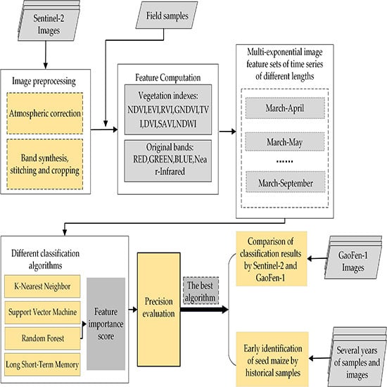
Field samples are necessary for use as reference data to train supervised classifiers for crops. They are also helpful for understanding the crop phenology calendar and planting conditions in the research area. In late July of 2017–2019, we carried out field research in Liangzhou. The sampling points were evenly distributed in the planting area. The collected data included crop types, growth situations, emasculation times of seed maize, plot areas, geographic coordinates, and field photos. In 2017, 48 ground-test samples were taken: 14 samples of seed maize, 18 samples of common maize, and 16 samples of other major crops (such as crown pear, grape, and spring wheat). In 2018, 385 ground-test samples were taken: 71 samples of seed maize, 162 samples of common maize, and 152 samples of other major crops. In 2019, 664 ground-test samples were taken: 160 samples of seed maize, 222 samples of common maize, and 282 samples of other major crops. The specific distribution of the samples is shown in Table 2 and Figure 2.

4. Methods

In this study, on the basis of crop type and phenological calendar differences in the study area, four aspects, namely biomass, chlorophyll content, soil background, and canopy water content, and eight indexes, namely NDVI, EVI, RVI, GNDVI, TVI, DVI, SAVI, and NDWI were selected as features. At the same time, we also added four original bands, namely red, green, blue, and near-infrared. The differences between different crops were compared in multiple dimensions to identify seed maize more effectively. From the different spectral reflectance of crops, Sentinel-2 10m images were used to construct the spectral curve of the eight vegetation indexes and four original bands of different crops. These features were then used to establish a feature image system to identify seed maize, and the influence of the time series length on the seed maize identification results was studied. Time series data of different lengths from March to September were used for modeling, and the accuracies of seed maize identification by KNN, SVC, RF, and LSTM were compared. In order to investigate the image quality of Sentinel-2, the classification accuracy was compared with that of GF-1. This study also extracted potential samples based on historical samples and clustering analysis method and then modeled and identified seed maize with time series data of different lengths. A flowchart detailing the process used in this study is shown in Figure 3. The methodology to extract new samples by historical samples section is shown in Figure 4.

4.1. Selection of Time Series Vegetation Indexes

Vegetation indexes are based on the spectral reflection characteristics of vegetation, combined with the visible and near-infrared bands of satellite images, and quantitatively reflect the growth and development of vegetation and soil background under certain conditions. These indexes are frequently used for regional and global land cover determination, vegetation classification, and growth monitoring [35,36]. According to the main crop types and their growing environment in the study area, the eight vegetation indexes in Table 3 were initially selected for analysis.
The main crop types in the study area include seed maize, common maize, spring wheat, crown pear and grape. The commonly used vegetation indexes provide information by using the spectral reflection difference of different vegetation, and their characteristics and the information that they provide differ: NDVI and EVI can reflect the comprehensive change in crop biomass. EVI has strong anti-saturation. When crop biomass is high, EVI is more sensitive to differences in biomass between crops; when the biomass is low, NDVI can better reflect the biomass difference between crops. TVI, RVI, and GNDVI can reflect the chlorophyll content of crops. The sensitivity of the three characteristics varies and is dependent on different growth and development stages of vegetation. DVI and SAVI can reflect the background of crop soil. DVI is sensitive to soil background changes due to different shading conditions of crops in different periods. With the increase in biomass, the value of DVI increases rapidly. SAVI explains the change in optical characteristics of soil background. NDWI can reflect the canopy moisture content of crops and the water content of vegetation canopy. When the vegetation canopy is subjected to water stress, NDWI can detect this quickly. Since many studies [29,32] have shown that the original spectral bands have a better effect on crop classification, this study added the original bands of red, blue, green, and nir in the feature set. The main research object of this paper was seed maize. Seed maize and common maize belong to maize, but their planting patterns are different (as shown in the Figure 5). The identification of other crops in the classification is mainly to improve the generalization ability of the model. According to expert knowledge, the biomass of seed maize is smaller than common maize in the whole growth period. As shown in Figure 6, NDVI and EVI of seed maize were lower than common maize in the whole trend, and the difference between them was more obvious from July to August when seed maize finished the female castration. There were differences in spectral reflectance profiles between seed maize and common maize, which indicated that seed maize and common maize could be classified.
A phenological calendar is a calendar that combines the phenology of plants with natural environmental conditions, such as climate and hydrology. Because of the different growth and development processes of different crops, the phenological calendars also differ among most crops; the phenological calendar of the main crops in the study area is shown in Figure 7. In this study, from the phenological calendars of the main crops in the study area—especially those of seed maize and common maize, which are more difficult to distinguish—time series remote sensing images captured during the main crop growth period in the study area were obtained, and the time series values of various vegetation indexes were calculated. The eigenvalues of the time series vegetation indexes corresponding to the field survey samples were extracted, and the time series characteristic curves of the vegetation indexes were constructed to reflect the process of crop growth and development.

4.2. Selection of Classification Algorithms

At present, many machine learning classification methods are applied to crop classification research, but no algorithm can solve all problems perfectly [45]. Therefore, we tried to find a suitable algorithm for the early identification of seed maize. This study aimed to test the performance of the algorithms through empirical judgment and classification accuracy. The four algorithms tested were K-nearest neighbor (KNN) [46], support vector classification (SVC) [47], random forest (RF) [48], and long short-term memory (LSTM) [49]. Based on these four algorithms, the data of different length time series from March to September in Liangzhou were modeled, and the effects of identification of seed maize under different time series lengths were compared. Furthermore, dynamic time warping (DTW) [50] was also used to establish the characteristic data set of the KNN algorithm. DTW is used to calculate the distance between different time series data, and this distance serves as the distance function in the nearest neighbor algorithm. SVC is a very powerful and flexible machine learning model that can perform linear or nonlinear classification and is widely used in crop classification research. The random forest algorithm is an integrated algorithm—a branch of machine learning—that can perform regression and classification. It can process input samples with high dimensional features without dimensionality reduction and can evaluate the importance of each feature in the classification process. This paper also used this algorithm to analyze the important characteristics in the early identification of seed maize. At present, many scholars have begun to use the deep learning algorithm to research crop classification and have achieved good results. The LSTM algorithm is suitable for processing time series data, so we selected LSTM and evaluated its performance in this experiment.

4.3. Experiment Design

We designed the following experiments to understand the performance of early identification of seed maize based on current or historical samples. Firstly, we established the feature system of eight vegetation indexes and four original bands based on the current samples and Sentinel-2 images. The data of different respective time series lengths from March to September were modeled. In addition, we compared the classification accuracy of KNN, SVC, RF, and LSTM to obtain the best classifier and the earliest time series for identification of seed maize. In order to verify the reliability of seed maize identification and the quality of Sentinel-2 images in this research, we conducted a time series progressive experiment based on the same features and the best classifier using GF-1 images. Because RF can evaluate the importance of each feature in the classification process, we also used this method to analyze the important features of different time series classification.
On this basis, we further made comprehensive use of historical samples and remote sensing data to generate new samples based on the k-means clustering method to realize early prediction of seed maize. A similar method has been successfully applied to the classification of maize and rice [51]. In this study, we improved the method and applied it to the early identification of seed maize. First, we used the samples from 2017 and 2018 to conduct ten crop mappings, superimpose classification results for 2017 and 2018, and calculate the frequency of different crop types per pixel. As the crop type frequency of this pixel was twenty times in 2017–2018 (ten classification results per year, a total of two years), the pixel was extracted as a potential sample. Then, according to the spectral characteristics and spatial information of images in 2019, the potential samples were clustered based on the k-means algorithm by the Google Earth Engine platform. Finally, we calculated the proportion of major crop types in each clustering item, and the crop category with the largest proportion was selected as the category of this clustering item; the clustering results were superposed with potential samples, and the pixels with the same category were extracted as new samples in 2019. Based on the new samples and the Sentinel-2 in 2019, the training of feature sets of different time series lengths from March to September was constructed to realize the early prediction of seed maize, and true samples from 2019 were used to evaluate the accuracy of this method. The method mainly considered the local stable planting structure and spectral information of the current year to realize the historical sample reuse and the early prediction of seed maize. Finally, we evaluated the accuracy of the classification results mainly through the confusion matrix and used the three metrics of overall accuracy (OA), producer accuracy (PA), and user accuracy (UA).

5. Results

5.1. Early identification of Seed Maize Based on the Current Samples

5.1.1. Early Identification by Different Algorithms

A multi-dimensional sample time series spectral feature set was constructed by using field research samples and obtaining time series Sentinel-2 images for the crop growth period (from March to September). Two-thirds of the research units were randomly selected as training samples, and the remaining part of the units were used as verification samples. For each algorithm, we conducted 10 experiments. The partition of each data set was based on Monte Carlo cross validation, in each experiment, and the training and verification data were randomly divided again at a ratio of 2:1.
KNN, SVC, RF, and LSTM were used for modeling and classification, and we chose the confusion matrix to evaluate the performance of models. The accuracies of crop classification, based on 10 repetitions, are shown in Table 4. Since the main research object of this paper was seed maize, we listed PA and UA for seed maize in the table. The comparison of overall accuracy is shown in Figure 8. According to the results, the classification accuracy of KNN, RF, and LSTM increased with the extension of time series. However, the classification accuracy of SVC began to decrease after it reached its peak in March to June. Through analysis, as the time series grew, more and more sentinel-2 images were added to the classification process, but the sample size remained unchanged, resulting in the problem of sample dilution, which led to subsequent precision reduction. The highest classification accuracy of both RF and LSTM reached more than 90%, and the PA and UA of seed maize exceeded 94%. On the whole, LSTM performed better than RF, indicating that the deep learning algorithm was indeed effective in crop identification research. In this experiment, we chose LSTM as the most suitable classifier. This could be seen from the classification accuracy diagram with different Sentinel-2 time series lengths. In March and April, most of the vegetation began to grow, wheat was just turning green, while crops such as maize were newly or not yet sown, and their biomass was usually low. After May, crops grew rapidly, and the spectral differences between crops in the remote sensing images increased; as a result, the classification accuracy increased rapidly. From June to September, with the increase in the time series length, on the whole, the classification accuracy of seed maize continued to improve. Moreover, by the end of June, the OA of classification could reach 89%, and the PA and UA of seed maize could reach over 90%. Although there was a slight drop in classification accuracy at the end of July, the impact was not significant. The distribution maps of seed maize based on LSTM with different time series lengths are shown in Figure 9. We found that seed maize was mainly distributed in the northwest and southeast corner of Liangzhou, which was also consistent with the actual situation. It also can be seen from the figures that seed maize was planted in clusters, because seed maize is a special crop and requires a high planting environment to produce relatively pure seeds. Comprehensive consideration of timeliness, economic cost, and classification accuracy suggests that it is more reasonable to carry out the early identification with the March–June time series by obtaining the remote sensing images from March to June in a timely manner and constructing the spectral feature image sets to identify the seed maize. This strategy was more consistent with the selection of the optimal time period in practice.
According to the characteristics of the random forest classification algorithm, the importance of classification features could be sorted. There are two ways to get the importance score of features in the random forest. One is based on Gini index and another is based on out-of-bag (OOB) error. We chose the second approach here. Our experiments were done using python and the rfpimp package [52], which is based on OOB. In this study, the RF algorithm based on time series feature sets of different lengths was used to conduct ten experiments. According to the ranking of the importance of each feature obtained by each experiment, we voted on each feature. Finally, the top ten features were selected by the average of the ranking scores comprehensively. Figure 10 shows the top ten features in this experiment with extension of time series. Feature importance ranking was done for March to April, March to May, and March to June. The features of DOY108 are high on the list, according to the phenological calendar. Seed maize at this time was just starting to be sown; common maize was seeded the most, spring wheat had entered a growth period, and crown pear had also just started to bud. Thus, at this time, the landscape of different crops and the growth difference were obvious. Adding images of July, seed maize and common maize entered a period of rapid growth, while spring wheat was in the harvest period, crown pear began to enter the harvest period, and the biomass began to decline. Therefore, the characteristics of DOY203 were relatively important. At the beginning of August, seed maize had completed the emasculation work, while seed maize and common maize had the most obvious difference; spring wheat had completed the harvest, crown pear had fully entered the harvest period, and grape had also begun to enter the harvest period. At this time, the growth difference of each crop reached the maximum. In September, most of the crops had been harvested, and the ground was exposed, so the importance score of the blue was getting higher.

5.1.2. Classification Comparison of Sentinel-2 and GF-1

In order to observe the reliability of the time series from March to June as the earliest period of seed maize and the image quality of Sentinel-2, we selected the medium-high resolution GF-1 images to do a contrast experiment based on the best effect classifier. In the experiment, two-thirds of the research units were randomly selected as training samples, and the remaining part of the units were used as verification samples. The comparison of accuracy results are shown in Figure 11. The classification accuracy based on Sentinel-2 was slightly higher than that of GF-1, indicating that the image quality of Sentinel-2 was reliable. Meanwhile, the classification accuracy based on GF-1 from March to June reached 85%. This shows that it was reasonable to choose images from March to June as the earliest identification time of seed maize.

5.2. Early Identification of Seed Maize Based on Historical Samples

In addition to timeliness, the economic cost and safety of field sampling were also considered in the early identification of seed maize. Furthermore, we tried to give consideration to the method of using historical samples to realize rapid identification. In this study, the model of the classification year was constructed based on historical data and image data, which generated new samples. This method was proposed because the planting structure of crops and seed maize fields were stable in the research area. Potential samples were extracted by the superposition of classification year image clustering results with the same crop type in historical years. We also considered the proportion of sample structure at the same time. In order to get clustering results quickly, the experiment was conducted on the Google Earth Engine platform. Finally, we used the new samples to implement crop classification with images of different time series lengths. The new samples are shown in Figure 12.
The newly generated samples were used as the training data of the classification model, and then one-third of the true samples was taken as the verification sample. The models were constructed based on the feature sets of different time series lengths, and the classification results were evaluated by the confusion matrix. The accuracy results are shown in Figure 13. On the whole, the classification accuracy increased with the extension of time series, and the classification accuracy of the full time series reached 74%. From March to July, the accuracy reached more than 60%, which could basically meet the requirements of related management departments for the early identification of seed maize. It can be seen from the results that there is a lot of potential for the use of historical samples. The full use of historical samples can save a lot of labor and material resources and improve the inter-annual generalization ability of models. The use of historical samples is also one of the important methods to realize large-scale rapid mapping.

6. Discussion

The paper evaluated the early identification of seed maize. As far as we know, many seed companies use UAV to distinguish crop phenotypes and genotypes. However, for this study, it was difficult to monitor such a wide range of distributed locations with UAV because the area of each successive seed maize field is from several dozen hectares to several hundred hectares. Moreover, the cruising ability of most UAVs is insufficient, and it is difficult to realize large-scale monitoring of seed maize. Therefore, remote sensing technology is a good choice to realize large-scale monitoring quickly and efficiently, and the spatial resolution of GF-1 and Sentinel-2 selected in this paper can support the identification of seed maize based on the average size of seed maize fields.
Compared with the previous studies on seed maize identification [3,4,5,6], seed maize identification must wait until August or even after harvest, which leads to a lag in information. The method used in this paper can obtain the area and space information of seed maize at the end of June, the OA of classification could reach 89%, and the PA and UA of seed maize could reach over 90%, so as to realize the large-scale rapid mapping of seed maize. In addition to the length of the time series, the algorithm of classification was further explored. At present, the ability of deep learning method is more and more prominent in the field of crop classification. The LSTM method used in this study had a good identification effect on seed maize. The highest classification accuracy could reach more than 90%, and the PA and UA of seed maize exceeded 94%. Moreover, the performance of LSTM in accuracy was also very stable. This result means that seed maize can be identified with high accuracy by obtaining Sentinel-2 images in the middle and early part of the growing season. Nonetheless, RNN may have some problems, such as the gradient explosion problem. Therefore, the classification model can be improved by combining it with the convolutional neural network (CNN) [53,54] in later seed maize identification. Because the deep learning method is sensitive to feature differences and has a strong learning ability, we think we can also use the deep learning algorithm to extract features.
Furthermore, previous methods [3,4,5,6] required a large amount of sample data, which cost a lot of labor power and material resources. Therefore, the full use of historical samples is of great significance for large-scale crop mapping, which can save a lot of cost, realize rapid mapping, and provide effective information for decision-making departments to make timely decisions. In this study, the historical samples were reused to generate new samples to realize the early prediction of seed maize. This approach has generally achieved satisfactory results. The classification accuracy of full time series feature sets is 74%, and that of feature sets from March to July is 63%, which meets the basic requirements of the regulatory authorities for early identification of seed maize. This approach effectively improved the utilization efficiency of historical data and provided a new idea for the continuous development of crop mapping in many regions lacking crop samples. We preliminarily tried k-means for the research on the generation of new samples by combining historical samples with spectral information. Moreover, generative adversarial networks (GAN) [55] has become one of the most promising methods in the field of unsupervised learning on complex distribution in recent years. It has great potential to be used to perform cluster analysis on remote sensing images in generating new samples, which can fully learn the phenological characteristics of crops and improve the sample purity. Although this study obtained high accuracy in early identification of seed maize, it is worth noting that there are also some limitations. The available images of Sentinel-2 and GF-1 data seem to be scarce. Fusion of multi-source data can enhance the temporal resolution. For example, satellite image data from platforms such as Sentinel-1 and Landsat 8 can be added for comparison and fusion research to achieve more time series image coverage within the monitoring range and make full use of crop phenology to improve the precision and reliability of remote sensing identification of seed maize. In addition to focusing on the accuracy of classification results, the efficiency of computer modeling is also an attractive issue. Remote sensing data, as big data, requires a huge amount of computing resources from preprocessing to the whole classification process. Cloud computing platforms like Google Earth Engine can be used to assist classification calculation. In this study, we used Google Earth Engine for data clustering in the classification year, which achieved efficient computing, rapid operation, and reasonable allocation of resources. Cloud computing is also a potential direction for the future development of crop classification.

7. Conclusions

The remote sensing identification of seed maize needs to distinguish differences in planting patterns and varieties of the same crop. The ability to identify a seed maize field in the middle and early part of the growing season is crucial for agricultural administration departments to carry out market supervision. The core idea of this paper is to explore the early identification of seed maize based on Sentinel-2 images, that is, how early can seed maize be identified and what accuracy is acceptable during the whole growth period. We discuss this question from three aspects: classification algorithm, data source, and historical samples. To this end, this study used Sentinel-2 and GF-1 images as data sources. Analysis of the spectral reflection characteristics of seed maize, common maize, and other surrounding crops in remote sensing images formed a multi-phase spectral feature system, and the method for the early identification of seed maize was explored. The main conclusions are as follows:
With the time series of feature set being extended, the identification accuracy of seed maize based on KNN, RF, and LSTM was higher. However, the SVC algorithm began to decrease after the classification accuracy reached the peak from March to June. As more and more sentinel-2 images were added, the sample dilution problem appeared in the SVC algorithm. Among the four classification algorithms, LSTM was selected as the most suitable classifier. The seed maize mapping of this experimental area could be carried out at the end of June, and the accuracy could meet the basic requirements of market supervision and regulation. In terms of data source, we compared the classification results of Sentinel-2 and GF-1. By analyzing the accuracy of Sentinel-2 and GF-1 images, Sentinel-2 was further confirmed to be a good choice of data in this study. From the perspective of historical samples, we found that the earliest identification of seed maize could be achieved in July. This discovery shows us the great potential of historical samples.
This paper makes comprehensive use of historical samples and remote sensing data to generate new samples as training data based on expert knowledge, and true samples are used as validation data. The approach has generally achieved satisfactory results. However, the amount of sample data is an important problem in the early identification of seed maize. For areas lacking samples, the task still faces significant challenges. Therefore, it is necessary for us to further study how to transfer the sample characteristics from one region to another region with the support of transfer learning.

Author Contributions

Conceptualization, Z.L., C.Z., S.L., and X.Z.; methodology, Z.L., D.L., and Y.Z.; formal analysis, T.R.; investigation, T.R. and L.Z.; resources, Z.L.; data curation, T.R., L.Z., and X.X.; writing—original draft preparation, T.R.; writing—review and editing, Z.L., Y.K., and T.R. All authors have read and agreed to the published version of the manuscript.

Funding

This research was funded by National Key Research and Development Program of China, grant number 2018YFD0100800.

Acknowledgments

The authors would like to give sincere thanks to the anonymous reviewers and editors for their useful advice and comments to help improve the quality of this paper.

Conflicts of Interest

The authors declare no conflict of interest.

References

  1. Zan, X.; Zhao, Z.; Liu, W.; Zhang, X.; Liu, Z.; Li, S.; Zhu, D. The Layout of Maize Variety Test Sites Based on the Spatiotemporal Classification of the Planting Environment. Sustainability 2019, 11, 3741. [Google Scholar] [CrossRef] [Green Version]
  2. Zhao, Z.; Zhe, L.; Zhang, X.; Zan, X.; Yao, X.; Wang, S.; Ye, S.; Li, S.; Zhu, D. Spatial Layout of Multi-Environment Test Sites: A Case Study of Maize in Jilin Province. Sustainability 2018, 10, 1424. [Google Scholar] [CrossRef] [Green Version]
  3. Liu, Z.; Li, Z.; Zhang, Y.; Zhang, C.; Huang, J.X.; Zhu, D.H. Seed Maize Identification Based on Time-Series EVI Decision Tree Classification and High-Resolution Remote Sensing Texture Analysis. Trans. CSAM 2015, 46, 321–327. [Google Scholar]
  4. Zhang, C.; Jin, H.; Liu, Z.; Li, Z.; Ning, M.; Sun, H. Seed maize identification based on texture analysis of GF remote sensing data. Trans. CSAE 2016, 32, 183–188. [Google Scholar]
  5. Zhang, C.; Tong, L.; Liu, Z.; Qiao, M.; Liu, D.; Huang, J. Identification Method of Seed Maize Plot Based on Multi-temporal GF-1 WFV and Kompsat-3 Texture. Trans. CSAM 2019, 50, 163–168, 226. [Google Scholar]
  6. Lin, Z.; Zhe, L.; Ren, T.; Liu, D.; Ma, Z.; Tong, L.; Zhang, C.; Zhou, T.; Zhang, X.; Li, S. Identification of Seed Maize Fields with High Spatial Resolution and Multiple Spectral Remote Sensing Using Random Forest Classifier. Remote Sens. 2020, 12, 362. [Google Scholar]
  7. Zhang, C.; Liu, J.; Su, W.; Qiao, M.; Yang, J.; Zhu, D. Optimal scale of crop classification using unmanned aerial vehicle remote sensing imagery based on wavelet packet transform. Trans. CSAE 2016, 32, 95–101. [Google Scholar]
  8. Liu, L.; Jiang, X.; Li, X.; Tang, L.L. Study on classification of agricultural crop by hyperspectral remote sensing data. J. Grad. Sch. Chin. Acad. Sci. 2006, 23, 484–488. [Google Scholar]
  9. Hao, P. Crop Classification Using Time Series Remote Sensing Data. Ph.D. Thesis, University of Chinese Academy of Sciences, Beijing, China, 2017. [Google Scholar]
  10. Yang, N.; Liu, D.; Feng, Q.; Xiong, Q.; Zhang, L.; Ren, T.; Zhao, Y.; Zhu, D.; Huang, J. Large-Scale Crop Mapping Based on Machine Learning and Parallel Computation with Grids. Remote Sens. 2019, 11, 1500. [Google Scholar] [CrossRef] [Green Version]
  11. Gómez, C.; White, J.; Wulder, M. Optical remotely sensed time series data for land cover classification: A review. ISPRS J. Photogramm. Remote Sens. 2016, 116, 55–72. [Google Scholar] [CrossRef] [Green Version]
  12. Immitzer, M.; Neuwirth, M.; Böck, S.; Brenner, H.; Vuolo, F.; Atzberger, C. Optimal Input Features for Tree Species Classification in Central Europe Based on Multi-Temporal Sentinel-2 Data. Remote Sens. 2019, 11, 2599. [Google Scholar] [CrossRef] [Green Version]
  13. Derksen, D.; Inglada, J.; Michel, J. Geometry Aware Evaluation of Handcrafted Superpixel-Based Features and Convolutional Neural Networks for Land Cover Mapping Using Satellite Imagery. Remote Sens. 2020, 12, 513. [Google Scholar] [CrossRef] [Green Version]
  14. Kussul, N.; Lavreniuk, M.; Skakun, S.; Shelestov, A. Deep learning classification of land cover and crop types using remote sensing data. IEEE Geosci. Remote Sens. Lett. 2017, 14, 778–782. [Google Scholar] [CrossRef]
  15. Zhang, Y. Research on the Method of Crop Area Measurement Based on GF-1 Remote Sensed Data. Master’s Thesis, Jilin University, Changchun, China, 2017. [Google Scholar]
  16. Zheng, L. Crop Classification Using Multi-Features of Chinese Gaofen-1/6 Satellite Remote Sensing Images. Ph.D. Thesis, University of Chinese Academy of Sciences, Beijing, China, 2017. [Google Scholar]
  17. Chang, D. Study on Temporal and Spatial Variation of Net Irrigation Water Demand of Regional Crops Based on Object-Oriented Classification of Remote Sensing. Master’s Thesis, Chinese Academy of Agricultural Sciences, Beijing, China, 2018. [Google Scholar]
  18. Teimouri, N.; Dyrmann, M.; Jørgensen, R. A Novel Spatio-Temporal FCN-LSTM Network for Recognizing Various Crop Types Using Multi-Temporal Radar Images. Remote Sens. 2019, 11, 990. [Google Scholar] [CrossRef] [Green Version]
  19. Zhou, T.; Pan, J.; Han, T.; Wei, S. Planting area extraction of winter wheat based on multi-temporal SAR data and optical imagery. Trans. CSAE 2017, 33, 215–221. [Google Scholar]
  20. Guo, J.; Wei, P.; Liu, J.; Jin, B.; Su, B.; Zhou, Z. Crop Classification Based on Differential Characteristics of H/α Scattering Parameters for Multitemporal Quad-and Dual-Polarization SAR Images. IEEE Trans. Geosci. Remote Sens. 2018, 56, 6111–6123. [Google Scholar] [CrossRef]
  21. Zhou, Y.; Luo, J.; Feng, L. DCN-Based Spatial Features for Improving Parcel-Based Crop Classification Using High-Resolution Optical Images and Multi-Temporal SAR Data. Remote Sens. 2019, 11, 1619. [Google Scholar]
  22. Sun, L.; Chen, J.; Guo, S.; Deng, X.; Han, Y. Integration of Time Series Sentinel-1 and Sentinel-2 Imagery for Crop Type Mapping over Oasis Agricultural Areas. Remote Sens. 2020, 12, 158. [Google Scholar] [CrossRef] [Green Version]
  23. Inoue, S.; Ito, A.; Yonezawa, C. Mapping Paddy Fields in Japan by Using a Sentinel-1 SAR Time Series Supplemented by Sentinel-2 Images on Google Earth Engine. Remote Sens. 2020, 12, 1622. [Google Scholar] [CrossRef]
  24. Xu, L.; Zhang, H.; Wang, C.; Zhang, B.; Liu, M. Crop Classification Based on Temporal Information Using Sentinel-1 SAR Time-Series Data. Remote Sens. 2019, 11, 53. [Google Scholar] [CrossRef] [Green Version]
  25. Zhong, L.; Gong, P.; Biging, G.S. Efficient corn and soybean mapping with temporal extendability: A multi-year experiment using Landsat imagery. Remote Sens. Environ. 2014, 140, 1–13. [Google Scholar] [CrossRef]
  26. Ozdogan, M. The spatial distribution of crop types from MODIS data: Temporal unmixing using Independent Component Analysis. Remote Sens. Environ. 2010, 114, 1190–1204. [Google Scholar] [CrossRef]
  27. Brown, J.C.; Kastens, J.H.; Coutinho, A.C.; de Castro Victoria, D.; Bishop, C.R. Classifying multiyear agricultural land use data from Mato Grosso using time-series MODIS vegetation index data. Remote Sens. Environ. 2013, 130, 39–50. [Google Scholar] [CrossRef] [Green Version]
  28. Zhan, Y.; Shakir, M.; Hao, P.; Zheng, N. The effect of EVI time series density on crop classification accuracy. Optik—Int. J. Light Electron. Opt. 2018, 157, 1065–1072. [Google Scholar] [CrossRef]
  29. Hao, P.; Zhan, Y.; Li, W.; Zheng, N.; Shakir, M. Feature Selection of Time Series MODIS Data for Early Crop Classification Using Random Forest: A Case Study in Kansas, USA. Remote Sens. 2015, 7, 5347–5369. [Google Scholar] [CrossRef] [Green Version]
  30. Hao, P.; Li, W.; Zheng, N.; Aablikim, A.; Ni, H.; Xu, S.; Fang, C. The Potential of Time Series Merged from Landsat-5 TM and HJ-1 CCD for Crop Classification: A Case Study for Bole and Manas Counties in Xinjiang, China. Remote Sens. 2014, 6, 7610–7631. [Google Scholar] [CrossRef] [Green Version]
  31. Hao, P.; Tang, H.; Chen, Z. Early season crop type recognition based on historical EVI time series. Trans. CSAE 2018, 34, 179–186. [Google Scholar]
  32. Cai, Y.; Guan, K.; Peng, J.; Wang, S.; Seifert, C.; Wardlow, B.; Li, Z. A high-performance and in-season classification system of field-level crop types using time-series Landsat data and a machine learning approach. Remote Sens. Environ. 2018, 210, 35–47. [Google Scholar] [CrossRef]
  33. Vorobiova, N.; Chernov, A. Curve fitting of MODIS NDVI time series in the task of early crops identification by satellite images. Procedia Eng. 2017, 201, 184–195. [Google Scholar] [CrossRef]
  34. Wang, Y. Development of Maize Seed Industry in Liangzhou District. China Seed Ind. 2015, 10, 40–41. [Google Scholar]
  35. Jiang, H.L.; Yang, H.; Chen, X.P.; Wang, S.D.; Li, X.K.; Liu, K.; Cen, Y. Research on Accuracy and Stability of Inversing Vegetation Chlorophyll Content by Spectral Index Method. Spectrosc. Spect. Anal. 2015, 35, 975–981. [Google Scholar]
  36. Wang, H.; Liu, C.; Cong, P.; Fu, Q. Agriculture drought monitoring remote sensing based on enhanced temperature vegetation dryness index. J. Arid Land Resour. Environ. 2018, 32, 165–170. [Google Scholar]
  37. Rouse, J.W. Monitoring the Vernal Advancements and Retrogradation of Natural Vegetation; NASA/GSFC: Prince George’s County, MD, USA; Texas A&M University: College Station, TX, USA, 1974; pp. 1–137.
  38. Liu, H.; Huete, A. A Feedback Based Modification of the NDVI to Minimize Canopy Background and Atmospheric Noise. IEEE Trans. Geosci. Remote Sens. 1995, 33, 457–465. [Google Scholar] [CrossRef]
  39. Pearson, R.L.; Miller, L.D. Remote mapping of standing crop biomass for estimation of the productivity of the shortgrass prairie. In Remote Sensing of Environment VIII; Willow Run Laboratories, Environmental Research Institute of Michigan: Ann Arbor, MI, USA, 1972; 1355p. [Google Scholar]
  40. Gitelson, A.; Kaufman, Y.; Merzlyak, N. Use of a green channel in remote sensing of global vegetation from EOS-MODIS. Remote Sens. Environ. 1996, 58, 289–298. [Google Scholar] [CrossRef]
  41. Broge, H.; Leblanc, E. Comparing prediction power and stability of broadband and hyperspectral vegetation indices for estimation of green leaf area index and canopy chlorophyll density. Remote Sens. Environ. 2000, 76, 156–172. [Google Scholar] [CrossRef]
  42. Jordan, F. Derivation of leaf-area index from quality of light on the forest floor. Ecology 1969, 50, 663–666. [Google Scholar] [CrossRef]
  43. Huete, R. A Soil Adjusted Vegetation Index (SAVI). Remote Sens. Environ. 1988, 25, 295–309. [Google Scholar] [CrossRef]
  44. McFeeters, K. The use of the normalized difference water index (NDWI) in the delineation of open water features. Int. J. Remote Sens. 1996, 17, 1425–1432. [Google Scholar] [CrossRef]
  45. Rahman, M.; Di, L.; Yu, E.; Zhang, C.; Mohiuddin, H. In-Season Major Crop-Type Identification for US Cropland from Landsat Images Using Crop-Rotation Pattern and Progressive Data Classification. Agriculture 2019, 9, 17. [Google Scholar] [CrossRef] [Green Version]
  46. Keller, M.; Gray, R.; Givens, A. A fuzzy k-nearest neighbor algorithm. IEEE Trans. Syst. Man Cybern. 1985, 15, 580–585. [Google Scholar] [CrossRef]
  47. Cortes, C.; Vapnik, V. Support-vector networks. Mach. Learn. 1995, 20, 273–297. [Google Scholar] [CrossRef]
  48. Breiman, L. Random forests. Mach. Learn. 2001, 45, 5–32. [Google Scholar] [CrossRef] [Green Version]
  49. Hochreiter, S.; Schmidhuber, J. Long Short-Term Memory. Neural Comput. 1997, 9, 1735–1780. [Google Scholar] [CrossRef] [PubMed]
  50. Keogh, E.; Ratanamahatana, A. Exact indexing of dynamic time warping. Knowl. Inf. Syst. 2005, 7, 358–386. [Google Scholar] [CrossRef]
  51. Zhang, L.; Liu, Z.; Liu, D.; Xiong, Q.; Yang, N.; Ren, T.; Zhang, C.; Zhang, X.; Li, S. Crop Mapping Based on Historical Samples and New Training Samples Generation in Heilongjiang Province, China. Sustainability 2019, 11, 5052. [Google Scholar] [CrossRef] [Green Version]
  52. Terence, P. GitHub Repository. Available online: https://github.com/parrt/random-forest-importances (accessed on 16 April 2020).
  53. Goodfellow, I.J.; Pouget-Abadie, J.; Mirza, M.; Xu, B.; Warde-Farley, D.; Ozair, S.; Courville, A.; Bengio, Y. Generative Adversarial Networks. In Advances in Neural Information Processing Systems; MIT Press: Cambridge, MA, USA, 2014; pp. 2672–2680. [Google Scholar]
  54. Wan, L.; Zhang, H.; Lin, G.; Lin, H. A small-patched convolutional neural network for mangrove mapping at species level using high-resolution remote-sensing image. Ann. GIS 2019, 25, 45–55. [Google Scholar] [CrossRef]
  55. Schmidhuber, J. Deep learning in neural networks: An overview. Neural Netw. 2015, 61, 85–117. [Google Scholar] [CrossRef] [PubMed] [Green Version]
Figure 1. Study regions. (a) Gansu province, China; (b) Location of the study region in Gansu province; (c) true-color Sentinel-2 image of Liangzhou.
Remotesensing 12 02140 g001
Figure 2. The spatial distribution of crop samples in Liangzhou in (a) 2017; (b) 2018; (c) 2019.
Remotesensing 12 02140 g002
Figure 3. Flowchart of the steps in the early identification of seed maize.
Remotesensing 12 02140 g003
Figure 4. New samples extracted by historical sample section.
Remotesensing 12 02140 g004
Figure 5. The photos of (a) seed maize with parents and mothers regularly planted alternately;(b) common maize, which is planted with the same hybrid variety.
Remotesensing 12 02140 g005
Figure 6. The time series curves and spectral reflectance profiles of seed maize and common maize using Sentinel-2 images. (a) NDVI; (b) EVI; (c) spectral reflectance profiles for seed maize and common maize.
Remotesensing 12 02140 g006aRemotesensing 12 02140 g006b
Figure 7. The phenological calendar of the main crops in the study area.
Remotesensing 12 02140 g007
Figure 8. Box plots of the overall accuracy for KNN, SVC, RF, and LSTM.
Remotesensing 12 02140 g008
Figure 9. Distribution mappings of seed maize based on different time series lengths in Liangzhou. (a) March–April. (b) March–May. (c) March–June. (d) March–July. (e) March–August. (f) March–September.
Remotesensing 12 02140 g009
Figure 10. Top ten features in different time series lengths. (a) March–April. (b) March–May. (c) March–June. (d) March–July. (e) March–August. (f) March–September.
Remotesensing 12 02140 g010
Figure 11. The comparison of accuracy based on Sentinel-2 and GF-1. (a) PA of seed maize. (b) UA of seed maize. (c) OA.
Remotesensing 12 02140 g011
Figure 12. The spatial distribution of the new samples including common maize, seed maize, and other crops, which were generated from historical samples combined with spectral information.
Remotesensing 12 02140 g012
Figure 13. Overall accuracy, PA, and UA of seed maize based on new samples for different time series lengths.
Remotesensing 12 02140 g013
Table 1. Satellite image parameters of the research area.
Satellite TypeBand Number Wavelength Range (µm)Spectral RegionSpatial Resolution (m)YearScene Acquisition Date (DOY)
GF-1 WFV10.45–0.52Blue16201868,69,72,104,110,122,134,147,192,208,225
20.52–0.59Green
30.63–0.69Red
40.77–0.89Nir
Sentinel-2 MSI20.45–0.52Blue102017113,163,223,243
30.54–0.58Green201863,68,83,98,108,138,148,163,168,173,193,213,238,253,263,268
40.65–0.68Red
80.78–0.90Nir201973,83,88,108,138,148,203,213,223,248,263,273
Table 2. Statistics on the field sample data.
Crop201720182019TotalPercent
Seed maize147116024523%
Common maize1816222240236%
other crops1615228245041%
Total483856641097
Table 3. Vegetation indexes selected in the study.
Vegetation IndexesEquations
Normalized difference vegetation index (NDVI)NDVI = (NIR − R) / (NIR + R) [37]
Enhanced vegetation index (EVI)EVI = 2.5*(NIR − R) / (NIR + 6R − 7.5B + 1) [38]
Ratio vegetation index (RVI)RVI = NIR / R [39]
Green normalized difference vegetation index (GNDVI)GNDVI = (NIR − G) / (NIR + G) [40]
Triangular vegetation index (TVI)TVI = 60*(NIR − G) − 100*(R − G) [41]
Difference vegetation index (DVI)DVI = NIR − R [42]
Soil regulation vegetation index (SAVI)SAVI = (1 + L)1(NIR − R) / (NIR + R + L) [43]
Normalized difference water index (NDWI)NDWI = (G − NIR) / (G + NIR) [44]
Note. B, G, R, and NIR are the reflectivity of blue, green, red, and near-infrared bands, respectively; L is the soil regulation parameter and has a value of 0.5.
Table 4. Accuracy of different classification algorithms.
Classification AlgorithmDTW-KNNSVCRFRNN(LSTM)
PA
March–April80.3% ± 1.2%90.7% ± 1.3%89.8% ± 1%90% ± 1.4%
March–May86.6% ± 1.6%94.5% ± 0.8%93.5% ± 1.2%93% ± 1.9%
March–June90.9% ± 1.2%97.7% ± 1.3%95.5% ± 1.1%95% ± 1.2%
March–July 90.7% ± 1.3%97.4% ± 2.3%95.9% ± 1.1%95.3% ± 1.6%
March–August92.6% ± 1.1%98.3% ± 1.9%95.7% ± 1.3%95.7% ± 1.3%
March–September92.5% ± 1.2%98.1% ± 2.1%95.9% ± 1.2%95.8% ± 1.1%
UA
March–April77.7% ± 1.4%82% ± 0.08%83.2% ± 1%88.2% ± 1.3%
March–May82.9% ± 1%79% ± 1.6%87% ± 1.5%90.9% ± 1.5%
March–June88.8% ± 1.2%73.8% ± 1%91.7% ± 0.9%93.2% ± 1%
March–July 89% ± 1.1%68.2% ± 1.5%91% ± 1.3%92.4% ± 1%
March–August90.5% ± 1.1%64% ± 1.2%93% ± 1.1%94.6% ± 1.1%
March–September91.2% ± 1%56.3% ± 1.2%94.5% ± 1.3%95.2% ± 1%
OA
March–April72.5% ± 1%79% ± 1.1%79.8% ± 1%81.6% ± 1.1%
March–May78.3% ± 0.8%81.8% ± 0.8%85.4% ± 0.8%87.1% ± 2.6%
March–June85.8% ± 0.9%82.4% ± 1.6%89.1% ± 1.1%89.4% ± 1%
March–July 85.2% ± 0.9%78.8% ± 2.4%89% ± 1.2%88.9% ± 1%
March–August89% ± 0.8%79.7% ± 3.3%91.2% ± 0.8%92.2% ± 1%
March–September89.3% ± 1.3%78.6% ± 1%91.7% ± 0.9%92.4% ± 0.8%

