Validation of the EGSIEM-REPRO GNSS Orbits and Satellite Clock Corrections
by
 ,
,
Andreja Sušnik
1,*, 
Andrea Grahsl
2,
Daniel Arnold
2,
Arturo Villiger
2,
Rolf Dach
2,
Gerhard Beutler
2 and
Adrian Jäggi
2 1
Geospatial Engineering, School of Engineering, Newcastle University, Newcastle upon Tyne NE1 7RU, UK
2
Astronomisches Institut, Universität Bern, 3012 Bern, Switzerland
*
Author to whom correspondence should be addressed.
Remote Sens. 2020, 12(14), 2322; https://doi.org/10.3390/rs12142322
Submission received: 19 June 2020
/
Revised: 10 July 2020
/
Accepted: 14 July 2020
/
Published: 19 July 2020
Abstract
:In the framework of the European Gravity Service for Improved Emergency Management (EGSIEM) project, consistent sets of state-of-the-art reprocessed Global Navigation Satellite System (GNSS) orbits and satellite clock corrections have been generated. The reprocessing campaign includes data starting in 1994 and follows the Center for Orbit Determination in Europe (CODE) processing strategy, in particular exploiting the extended version of the empirical CODE Orbit Model (ECOM). Satellite orbits are provided for Global Positioning System (GPS) satellites since 1994 and for Globalnaya Navigatsionnaya Sputnikovaya Sistema (GLONASS) since 2002. In addition, a consistent set of GPS satellite clock corrections with 30 s sampling has been generated from 2000 and with 5 s sampling from 2003 onwards. For the first time in a reprocessing scheme, GLONASS satellite clock corrections with 30 s sampling from 2008 and 5 s from 2010 onwards were also generated. The benefit with respect to earlier reprocessing series is demonstrated in terms of polar motion coordinates. GNSS satellite clock corrections are validated in terms of completeness, Allan deviation, and precise point positioning (PPP) using terrestrial stations. In addition, the products herein were validated with Gravity Recovery and Climate Experiment (GRACE) precise orbit determination (POD) and Satellite Laser Ranging (SLR). The dataset is publicly available.

1. Introduction
Within the framework of the European Gravity Service for Improved Emergency Management (EGSIEM) [1] project, different monthly gravity field solutions derived from the Gravity Recovery and Climate Experiment (GRACE) [2] mission were compared and combined [3,4]. The main objective of the project was to demonstrate that the observations of the redistributions of water and ice mass, as derived from GRACE inter-satellite ranging, provide critical and complementary information to more traditional Earth observation data, e.g., optical or radar measurements. A consistent use of reference frame products (Earth rotation parameters (ERP), Global Positioning System (GPS) satellite orbits and clock corrections) at all EGSIEM processing centers was a prerequisite for comparability of the precise GRACE orbits, and the gravity fields derived thereof. The reference frame products provide the link between the geometrical (station coordinates) and physical (gravity field) shape of the Earth. For kinematic precise orbit determination (POD) of Low Earth Orbiting (LEO) satellites such as GRACE, precise point positioning (PPP) [5] is a well-established technique. However, the procedure requires precise and more importantly, consistent GPS orbits and satellite clock corrections. The Center for Orbit Determination in Europe (CODE) [6] started to generate GPS clock corrections with a 30 s sampling rate as early as 1999 [7] and with a 5 s sampling rate in 2008 [8].
Since the establishment of the International GNSS Service (IGS) [9,10] in 1994, global navigation satellite system (GNSS) data from the IGS tracking network have been analyzed on an operational basis by the global analysis centers (AC), including the CODE consortium, providing GPS- and Globalnaya Navigatsionnaya Sputnikovaya Sistema (GLONASS)-based products (satellite orbits, ERPs, station coordinates, troposphere parameters, ionosphere models, and clock corrections) on a daily basis. Over the years, models and methods to analyze the data have continuously improved. The changes in the processing scheme have led to inhomogeneous products, resulting in discontinuities within the time series of the solutions (e.g., they are not consistent in time, as was desired for the purposes of the EGSIEM project). Among others, [11,12] have shown that homogeneously reprocessing of GNSS observations leads to significantly improved products. When the EGSIEM project started in 2015, the most recent reprocessing campaign in the frame of the IGS (repro02, henceforth IGS-repro02) [13] was carried out in 2013–2014 to support the generation of IGS14 (an IGS-specific realization of the ITRF2014 reference frame) [14], which has been in use within the IGS since January 29, 2017 (GPS week 1934). However, neither the operational nor the IGS-repro02 series extended by the most recent years were optimal for the purposes of the EGSIEM project. Even though IGS-repro02 provided the latest homogeneously reprocessed products at that time, it was reported by [13] that the combined satellite clock corrections from different AC’s are severely limited by large residual biases and incompatible satellite attitude models adopted by different AC’s; therefore, the IGS-repro02 clocks should not be used for long-term PPP reprocessing, as was required by the EGSIEM project. Thus, a dedicated reprocessing series was required, offering the opportunity to take new models into account (e.g., an updated solar pressure model) [15].
To provide state-of-the art reference frame products, not only to the EGSIEM project but also for the wider GNSS community, the Astronomical Institute of University of Bern (AIUB) initiated a new reprocessing campaign in 2015 (henceforth EGSIEM-REPRO), covering the period between 1994 and 2014, with the addition of GLONASS (from 2002 onwards) to the GPS-based products. Consistent satellite clock corrections were generated for both GNSS systems. The final set of products is publicly available at ftp://ftp.aiub.unibe.ch/REPRO_2015/, and consists of ERPs, GNSS orbits and clock corrections, station coordinates, and troposphere parameters.
2. Materials and Methods
To generate a consistent set of GNSS products, data from more than 250 globally distributed stations were homogeneously processed for the time period 1994–2014. When the reprocessing was initiated, IGb08 [16,17] was still in use, together with the related antenna phase center corrections. Consequently, no change was necessary in the station selection with respect to the IGS-repro02 contribution from CODE. The reprocessing includes data starting on January 2, 1994, by analyzing only GPS data, and ending on December 31, 2014. GLONASS was included in the processing of data starting from January 1, 2002. A rigorously combined processing scheme using GPS and GLONASS measurements was used, according to the processing standards applied for the IGS activities at CODE [6]. A detailed description of measurement models and estimated parameters in the reprocessing can be found at http://ftp.aiub.unibe.ch/REPRO_2015/CODE_REPRO_2015.ACN.
The latest development version of the Bernese GNSS software [18] was used, together with the extension of the empirical CODE orbit model (ECOM2), adding periodic terms in the satellite–Sun direction [15]. The additional ECOM terms are of importance for satellites with elongated bodies, such as GLONASS. Table 1 summarizes the estimated parameters for the original (D0B1) and extended version of ECOM, where the 2- and 4 cycles-per-revolution (cpr) terms in the satellite–Sun direction are omitted (D4B1). The latter was used and applied for EGSIEM-REPRO. The parametrization type D2B1 represents a modified version of the extended ECOM (see Section 4).
In all three realizations of the ECOM, a Sun-oriented orthogonal coordinate system is used. The D component points from the satellite to the Sun, the Y component goes along the solar panel axis, and the B component completes a right-handed orthogonal system. For more information on the ECOM model, please refer to [15]. The extended ECOM model has been used for the IGS-related GNSS processing at CODE since January 4, 2015 [6,19].
2.1. Generation of GNSS Orbits
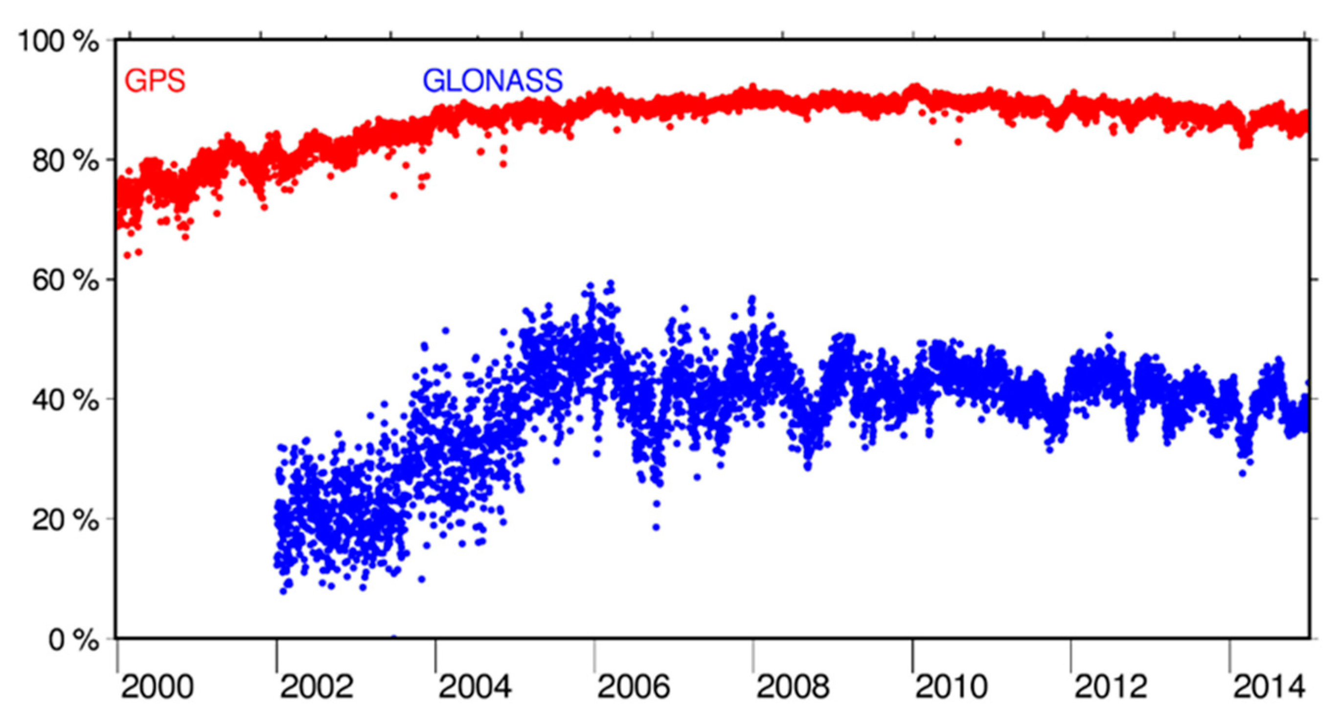
The processing chain starts with the generation of 1-day GNSS orbits based on a double difference approach. This implies that both station and satellite clock parameters are implicitly pre-eliminated. Normal equations (NEQs) containing GNSS satellite orbit parameters, ERPs, station coordinates, and troposphere zenith path delay parameters are set up and stored. An important aspect for obtaining high-quality GNSS products is the resolution of the carrier-phase double difference ambiguities to their integer values, since this procedure reduces the number of unknown parameters, and therefore improves the redundancy of the solution [20]. In other words, the solution becomes more stable. The ambiguity resolution is not only applied for GPS, but also for GLONASS [21]. Figure 1 shows the success rates of the ambiguity resolution for GPS and GLONASS. The increasing number of resolved ambiguities for GLONASS between 2002 and 2008 is related to the completion of the GLONASS tracking network, which achieved global coverage between 2006 and 2008. The limitation to 40% of resolved ambiguities for GLONASS is related to the fact that only ambiguities belonging to the same frequency are solved for baselines longer than 200 km.
Before combining 1-day NEQs into a 3-day solution, a consistency test is performed by fitting the satellite positions of three subsequent 1-day orbits to a 3-day orbital arc, represented by one set of orbit parameters over the three days. If the three subsequent orbits cannot be represented by one orbital arc with sufficient quality, the 3-day arc is split at the day boundaries. Such arc splits are introduced if the offset at the day boundaries is above a threshold of 4 times the arithmetic mean Root-Mean-Squared (RMS) value, which is computed with respect to all accepted satellites of a specific GNSS. This happens in less than 1% of all cases (e.g., when a satellite maneuver has taken place during the time period in question). In such a case, the long-arc strategy, if not properly handled, would degrade the solution.
Additionally, validation of the station-related parameters is performed in order to detect stations with discontinuities between subsequent days (e.g., due to equipment changes or earthquakes), before they can be connected to one set of coordinate parameters over three days. If such a station is detected, it is pre-eliminated for that day, preventing its contribution to the 3-day coordinate solution.
After these preparatory steps, three subsequent NEQs are combined into one NEQ and a 3-day long-arc solution is invoked [22]. The middle day is then extracted to represent the 3-day orbit referring to one particular day. The station coordinates, troposphere parameters, ERPs, and GNSS satellite orbits are obtained based on a minimum constraints solution (with a no-net-rotation condition applied) aligned to the IGb08 reference frame, while keeping the inner geometry of the GNSS solution. Before the final solution is generated, the stations used for datum definition are validated by checking the residuals of a Helmert transformation to IGb08, with a residual threshold of 10 mm for horizontal and 30 mm for vertical components.
2.2. Generation of Gnss Clock Products
The results from the double difference processing, described in the previous section, are then introduced as known parameters in the generation of the GNSS clock products. Here, in the first step a zero-difference network solution is performed, where all satellite and receiver clock parameters are estimated with a sampling rate of 300 s. The 300 s clock solution is then the basis for the efficient high-rate clock interpolation (EHRI) procedure using carrier-phase time-differenced measurements [8]. The changes of the receiver and satellite clock corrections from one epoch to the next are based on an epoch difference solution and fitted to the 300 s clock solution. As a reference clock, the station with the lowest RMS error in the linear fit and the most complete data is chosen daily.
This procedure is limited to a sampling rate of 30 s, since the standard IGS stations provide data only with this sampling rate, while for a further densification of the clock corrections GNSS observation files with a higher sampling rate are needed. GNSS data with a sampling of 1 Hz are available from the IGS real-time project [23].
In [8], it is shown that the high-rate GPS satellite clock corrections with 5 s sampling may be linearly interpolated, resulting in less than 2% degradation of accuracy. Figure 2 shows the number of stations delivering high-rate Receiver Independent Exchange Format (RINEX2) [24] data for the period between 2003 to the end of 2014. The number of stations increases from about 40 in 2003 to around 115 stations in 2014.
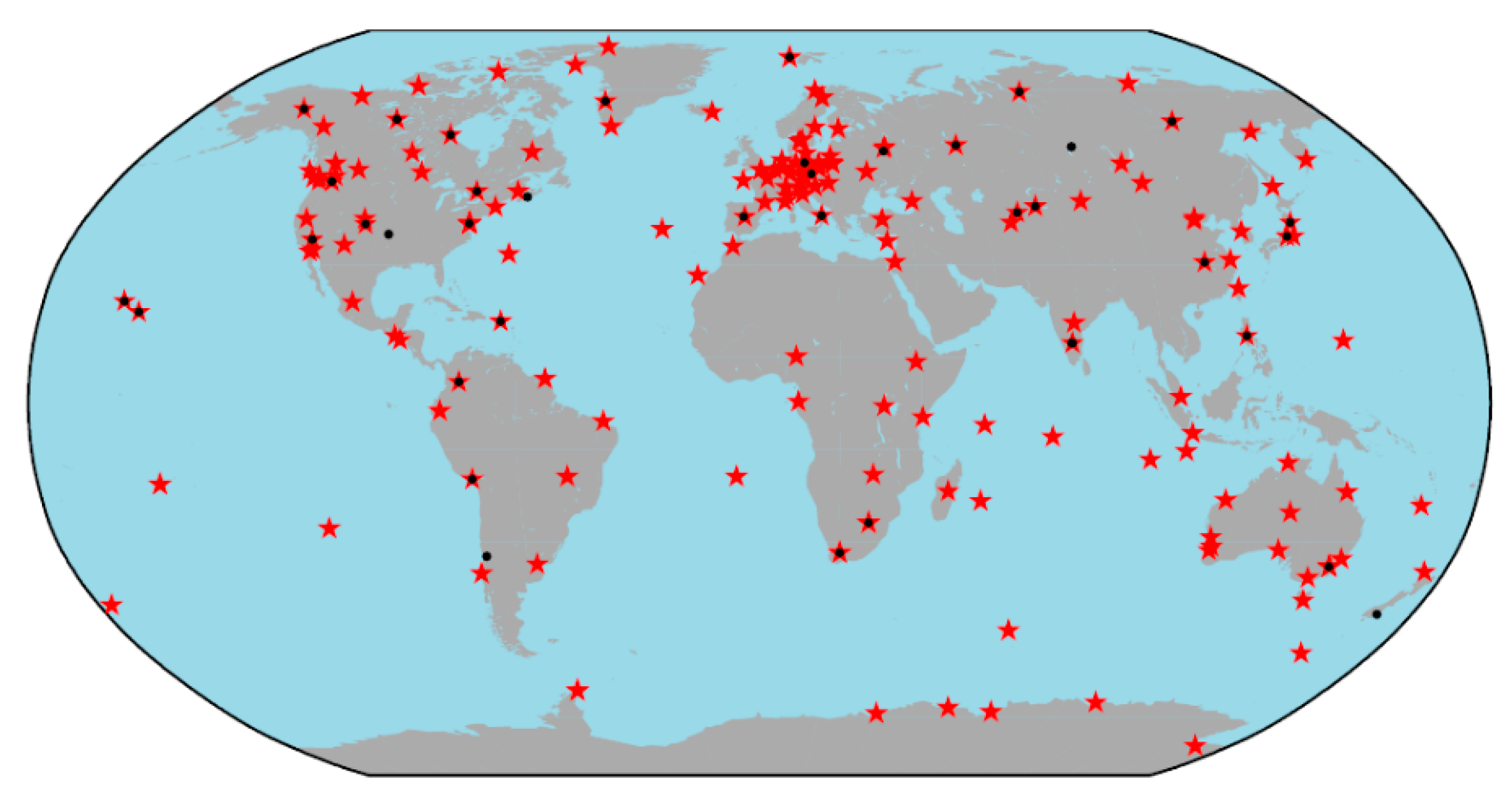
Their geographical distribution is of particular importance for obtaining GNSS satellite clock corrections that are as complete as possible. Figure 3 shows the geographical distribution of the stations delivering high-rate RINEX data for two selected days—January 1, 2003 (black dots), and January 1, 2014 (red stars). As can be seen, besides the increasing number of GNSS stations, the geographical coverage also significantly improves over the years. The coverage over the ocean is, however, not yet dense enough. Consequently, the completeness of the satellite clocks over these areas heavily depends on the availability and completeness of observations from a few stations.
In the frame of the EGSIEM-REPRO campaign, the procedure to densify the satellite clock corrections to 5 s sampling for the GLONASS satellites was performed for the first time in a reprocessing scheme. Finally, the GPS satellite clock corrections are provided in this reprocessing series with a sampling rate of 5 s from 2003 onwards. For GLONASS, the determination of complete satellite clock corrections started with data referring to year 2008 with 30 s sampling and in with 2010 data with 5 s sampling.
3. Results
The EGSIEM-REPRO and CODE contributions to the IGS-repro02 products were validated in six different ways. Section 3.1 analyzes polar motion misclosures with the methods originally proposed by [25]. Section 3.2 validates the GNSS satellite clock corrections in terms of the completeness and Allan deviations. In Section 3.3, the results of PPP analysis using terrestrial stations are presented and discussed. Section 3.4 makes use of the Satellite Laser Ranging (SLR) observation technique for validation of the GNSS orbits by calculating the measured SLR distances to GNSS satellites using the reprocessed GNSS orbits and satellite corrections, as well as the corresponding ERPs and the known locations of the SLR observatories, and applies the reprocessing products to generate the orbits of the GRACE satellites and validates the LEO orbit quality as a function of the reprocessing products.
3.1. ERP Misclosures
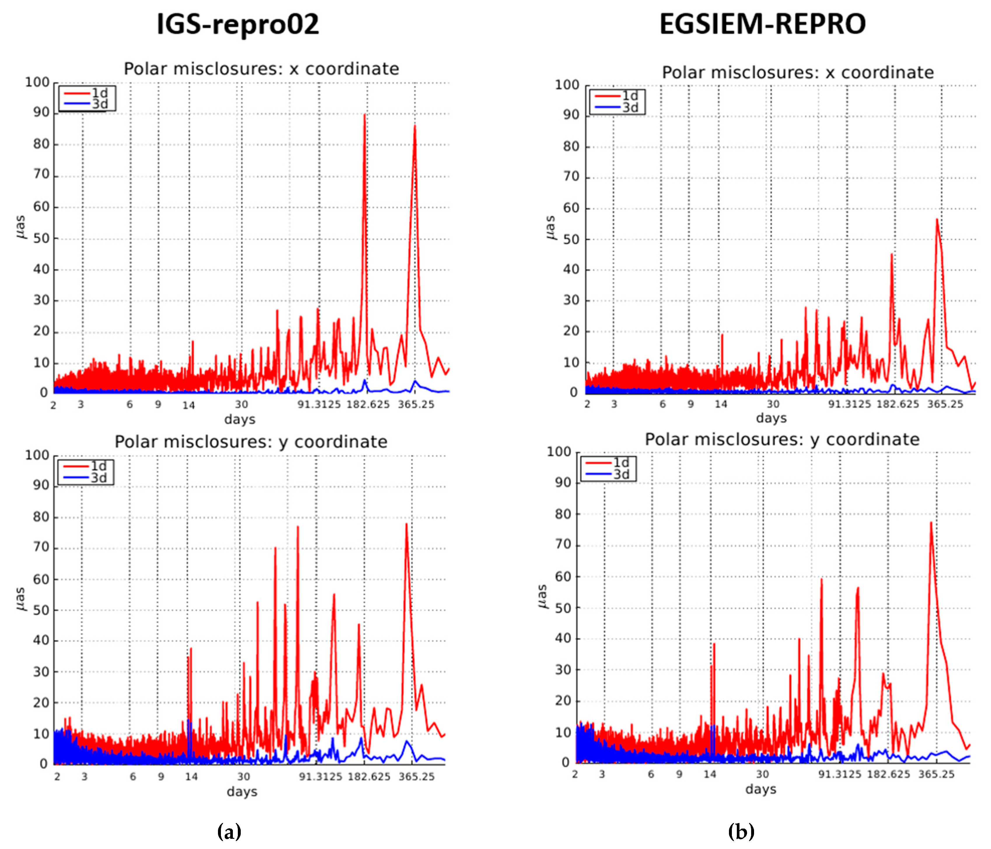
The polar motion misclosures at the day boundaries were calculated according to Equation (1) in [25]. One misclosure value result is used from each day for each of the polar motion coordinates x and y.
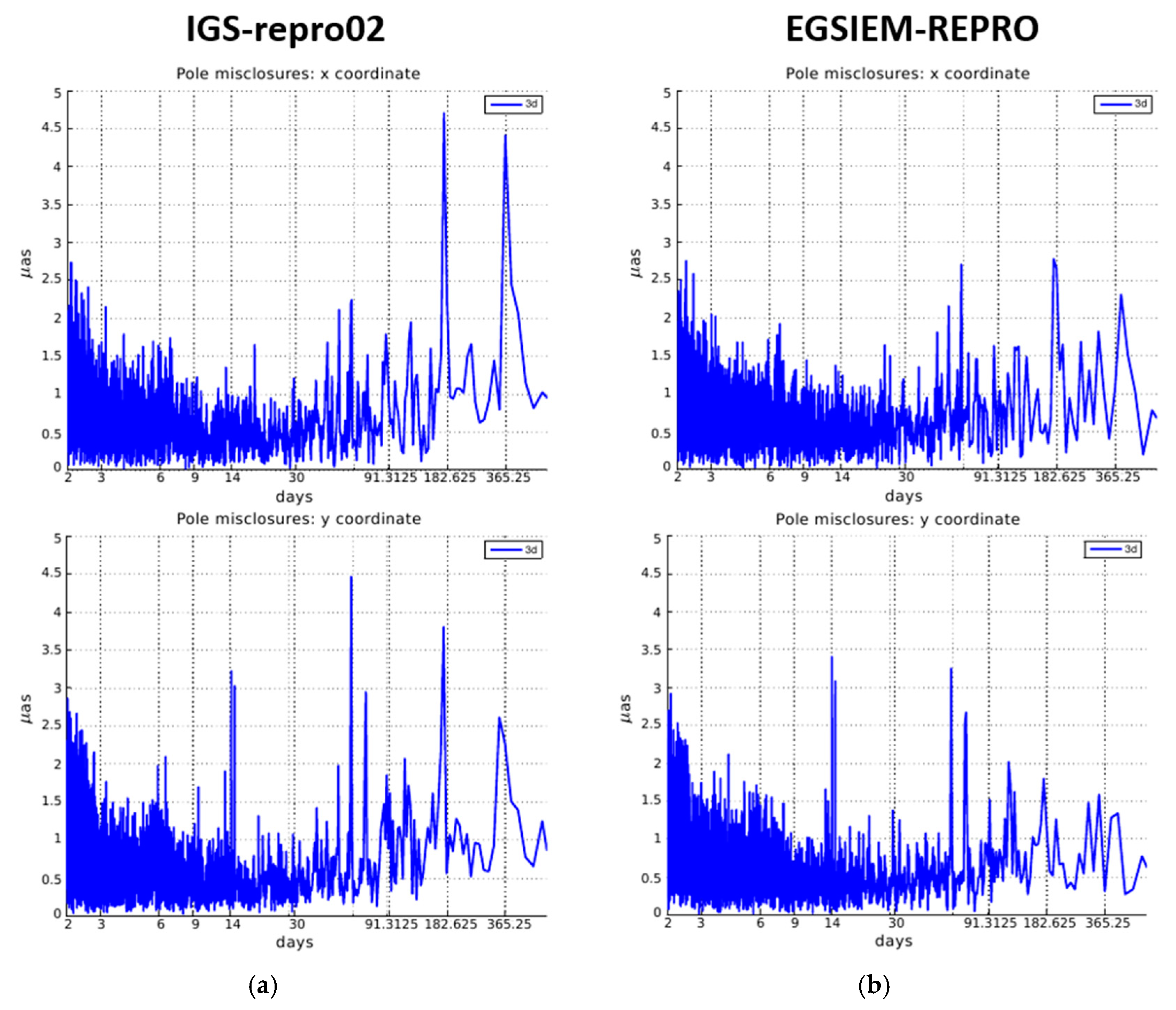
Figure 4 shows the polar motion misclosures, where the left column refers to the IGS-repro02 series and the right side to the EGSIEM-REPRO series. In Figure 4, the top row displays the x misclosures and bottom row displays the y misclosures. The figure clearly demonstrates the superiority of the 3-day solutions (shown in blue) over the 1-day solutions (shown in red). On the other hand, it is difficult to decide which of the two series (e.g., EGSIEM-REPRO and IGS-repro02) with the same arc length is better. For this reason, Figure 5 shows the spectra of the polar motion series of Figure 4, providing greater insight, at least for the 1-day solutions. As opposed to Figure 4, which cover the time interval 1994–2013, the spectra are based on the misclosures in the time interval 2000–2014, thus excluding the solutions that are still far from present-day quality.
Figure 5 reveals that the EGSIEM-REPRO series is superior to the IGS-repro02 series—the amplitudes of the spectral lines of the 1-day solutions for periods > 30 days are greatly reduced in the right side of Figure 5 compared to the left side of Figure 5, while the amplitudes in y with the period of one year are an exception, which are almost the same in both daily misclosure series. In order to assess the quality of the 3-day solution’s power spectrum shown in Figure 5, this is plotted by skipping 1-day solutions, as presented in Figure 6. As can be seen, the amplitudes are greatly reduced from Figure 5 to Figure 6 by a factor of approximately 50 or more. The figures also show the superiority of the EGSIEM-REPRO series with respect to the IGS-repro02 series; for periods between 30 and 600 days, the amplitudes are substantially smaller for the EGSIEM-REPRO series. The amplitudes in this domain of periods represent a good quality criterion, since the spurious effects due to radiation pressure deficiencies in the orbits are expected to be seen.
Table 2 summarizes the statistical properties of the polar motion misclosures for different ranges of periods. The normal RMS is provided with the label “all”, whereas the RMS referring to periods <30 days is labeled “<30” and the RMS referring to the periods between 30 and 600 days is labeled “30 < P < 600”. The latter value is important, as it characterizes the amplitudes of the spurious spectral lines associated with the draconitic year and its harmonics. In this domain, the EGSIEM-REPRO RMS values are about 20–30% smaller for the 1-day solutions and about 10–20% smaller for 3-day solutions. Note, however, that the absolute values are small (1 mas corresponds to 31 mm on the surface of the Earth, and to 128 mm at the altitude of GPS satellites).
3.2. GNSS Satellite Clock Corrections Analysis
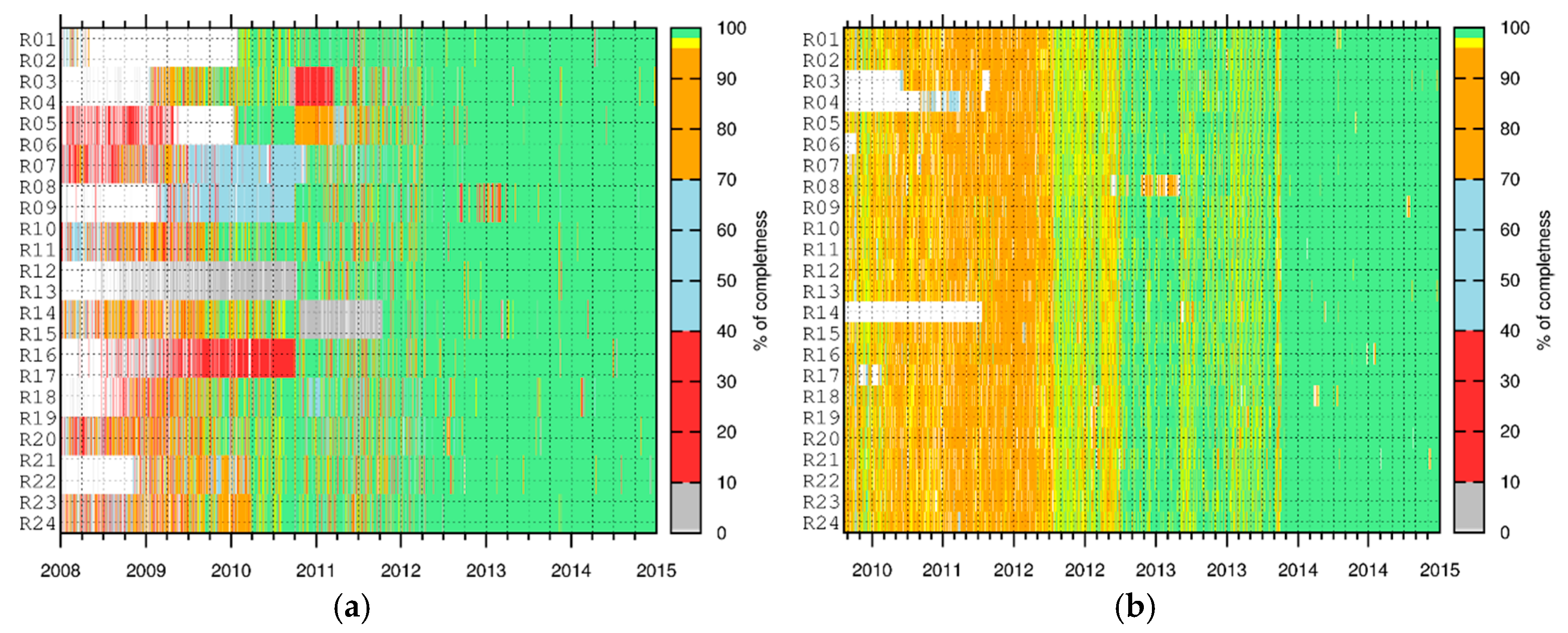
As the first quality control measure, the completeness of the GNSS clock corrections was checked separately for the 300, 30, and 5 s clock corrections for both GPS and GLONASS. As an example, Figure 7 shows the completeness of the GLONASS satellite clock correction with 30 s (Figure 7a) and 5 s (Figure 7b) sampling rates. Note that the time scales for the figures are different due to the fact that GLONASS satellite clock corrections with 30 s sampling are available from 2008 onwards, while the 5 s GLONASS satellite clock corrections are available from 2010 onwards. It can be noticed that the completeness of the 30 s clock corrections increases with time, reaching 100% at the beginning of 2010 for the majority of the satellites. The data gaps, which are visible for some satellites, are mainly due to the reduced ground tracking network. Additionally, the full constellation for GLONASS was not achieved until 2014; therefore, not all pseudorandom noise numbers (PRN) were constantly in use.
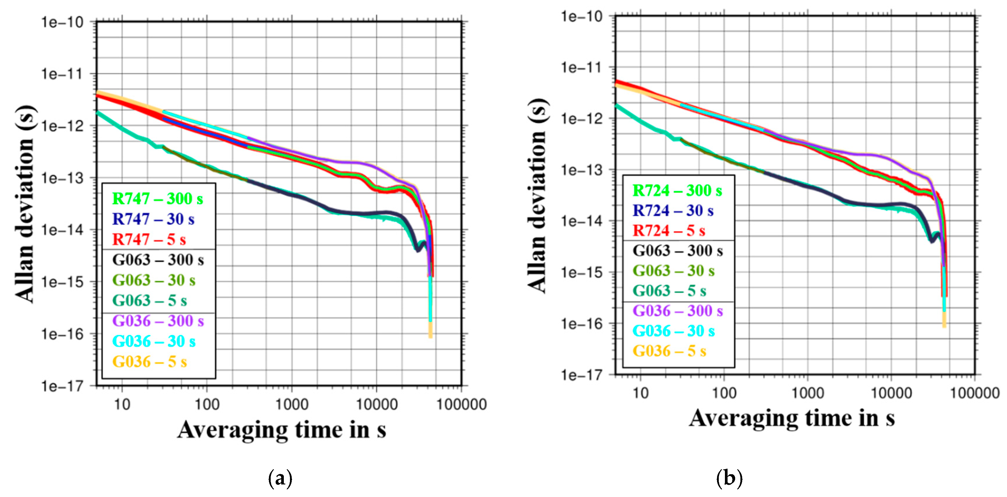
Since the GLONASS satellite clock corrections with 5 s sampling were calculated for the first time in the reprocessing mode, their quality was investigated in more detail, particularly to see if the clock determinations with 300 s, 30 s, 5 s sampling had any impact on the quality of the GLONASS satellite clock corrections. Figure 8 shows an example of Allan deviations (ADEV) [26] of the satellite clock corrections with different samplings for selected satellites on 27 October 2013. While both of the GLONASS satellites, R724 (Figure 8a) and R747 (Figure 8b), are GLONAS-M types with cesium on-board clocks, the GPS G063 satellite is a Block-IIF type and the G036 satellite is a Block IIA type, both with rubidium on-board clocks. As can be seen from Figure 8, the lines for all three solutions are the same, implying that the densification process works very well for interpolation.
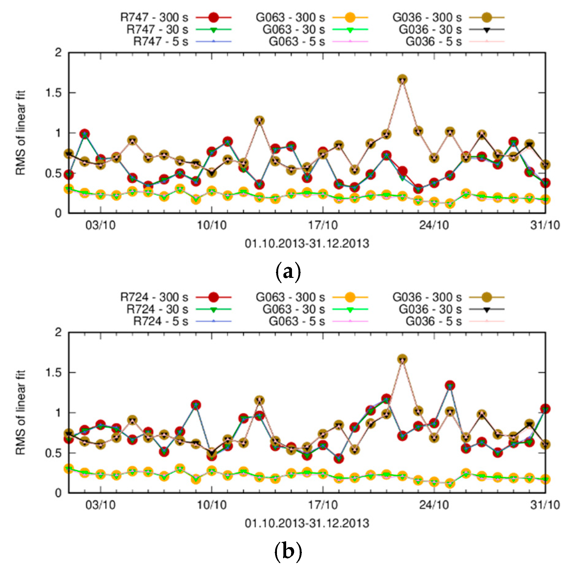
Another performance indicator for GNSS satellite clocks is the RMS of the daily linear fit through the epoch-wise clock estimates. This characterizes how close a clock comes to the ideal linear drift. The daily RMS fit of the estimated clocks for selected GPS and GLONASS satellites is shown in Figure 9. Here, the same satellites are shown as in Figure 8.
As can be seen from Figure 9, in terms of the daily RMS of the linear fit, the best performing clock is G063, which is expected since the satellite belongs to the youngest type of satellites. There is no noticeable difference when comparing both selected GLONASS satellites. On the other hand, it appears that they both perform better than the G036 satellite. Overall, there is no visible difference between the different solutions with different samplings.
In order to further evaluate the products, particularly the GLONASS satellite clock corrections, we performed ground-based PPP for a selected period and for selected stations for the year 2013. The reason for the selected period is the fact that in 2013 GLONASS reached its full constellation, hence satellite clock corrections were 100% complete for this year. For the station selection, the following criteria had to be fulfilled: (1) the station had to track both GPS and GLONASS satellites; (2) it had to provide RINEX2 data with 5 s sampling; and (3) the station had to be driven by a hydrogen maser receiver clock. Three different solutions were generated based only on the phase measurements, namely:
- GPS + GLONASS kinematic solution;
- GPS only kinematic solution;
- GLONASS only kinematic solution.
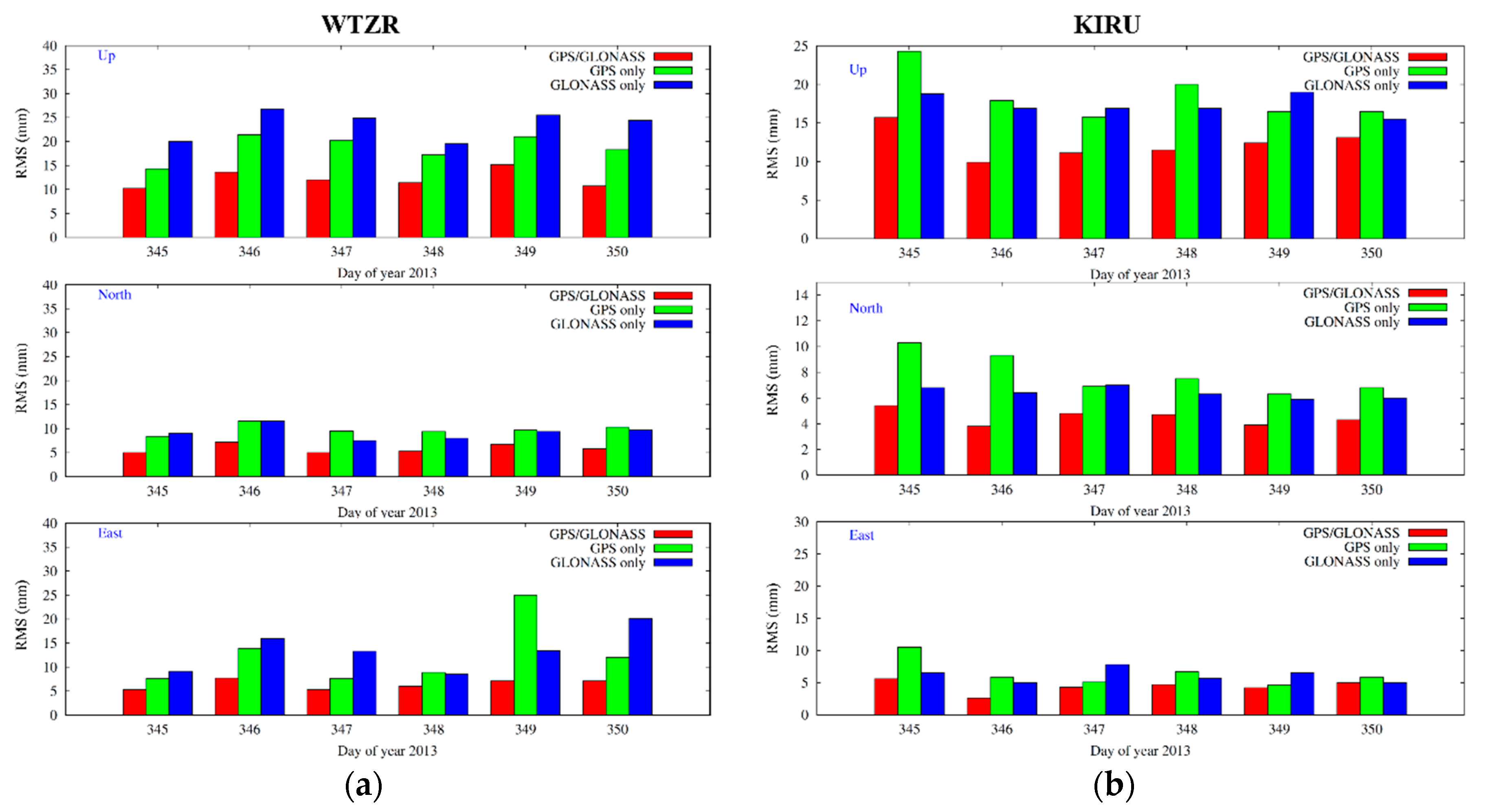
The right side of Figure 10 shows daily RMS values of the coordinate residuals with respect to the a priori coordinates in the north, east, and up components for WTZR station (Wettzell, Germany). As expected, the GLONASS only solution has the worst performance, since the number of satellites is still lower than GPS by about 25%. However, looking at Figure 10a, one can notice that the GLONASS only solution performs better in the north component than with GPS. One possible explanation for this is that the WTZR station is located at +49.08 latitude, therefore having better GLONASS satellite geometry than GPS, since GLONASS has a higher inclination (64.8°) with respect to GPS (55°). In order to confirm this, an additional PPP solution was calculated for KIRU station, which is located in Kiruna, Sweden. The results are shown on the left side of Figure 10, where one can see that GLONASS shows better repeatability in the north component than GPS.
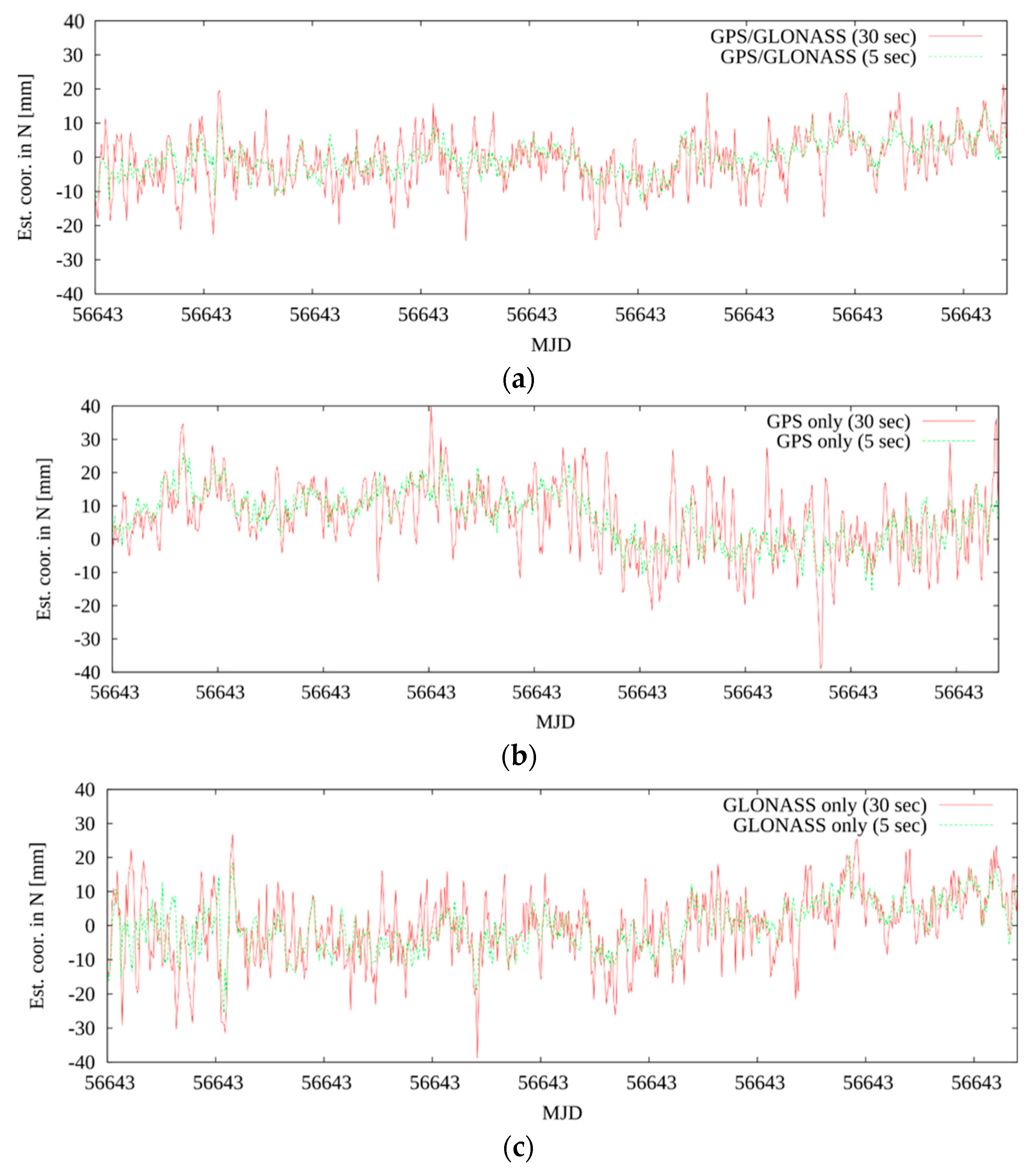
In the last step of the GNSS satellite clock corrections evaluation, the PPP solution was generated, for which we used GNSS satellite clock products with 30 s sampling interpolated to 5 s in the PPP procedure. Figure 11 shows estimated kinematic coordinates for the north component obtained using different sampling approaches for the first hour on December 17, 2013. On the top of Figure 11 the GPS+GLONASS solution is shown, the middle presents the GPS only solution, while the bottom shows the GLONASS only solution. The corresponding Allan deviations for the full day, all three components, and the GLONASS only solution are presented in Figure 12.
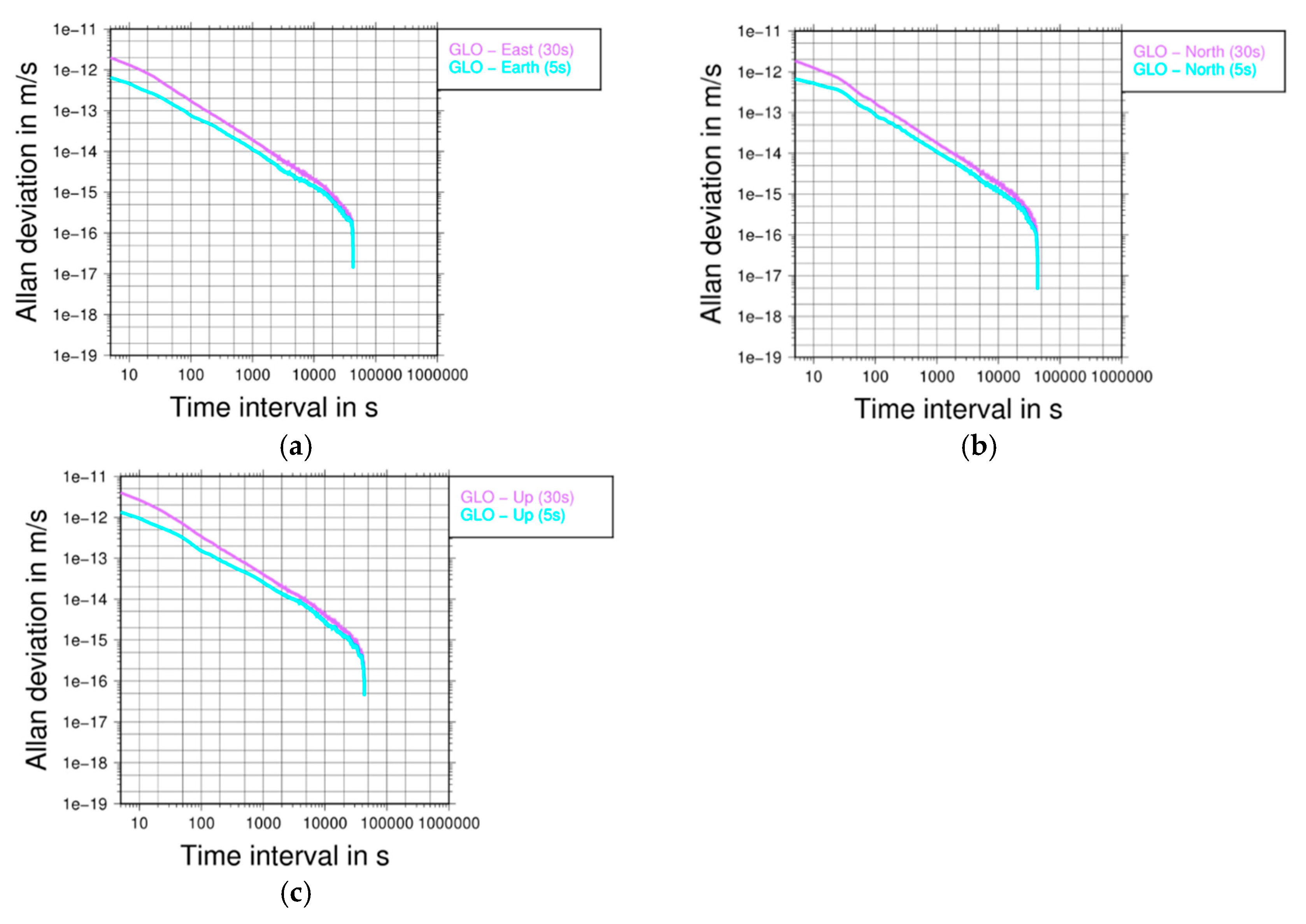
Looking at Figure 11, it can be noticed that all solutions obtained with 5 s satellite corrections show less noise than the solution with 30 s satellite corrections that were then interpolated to 5 s. In particular, this can be confirmed by looking at the Allan deviation results for the estimated kinematic coordinates shown in Figure 12. Here, the Allan deviation was calculated over the entire day for the GLONASS only solutions.
3.3. Validation of GNSS Orbits by Satellite Laser Ranging
Satellite Laser Ranging (SLR) to spacecraft equipped with laser retroreflectors always yields highly precise and unambiguous distance measurements between laser stations and the spacecraft. All GLONASS satellites carry retroreflectors, and thus can be tracked by SLR. Two GPS satellites equipped with retroreflectors were decommissioned, namely G036, which launched on March 10, 1994, and was decommissioned in 2014; and G035, which launched on August 30, 1993, and was decommissioned in 2009 [27]. Since the reprocessed GLONASS and GPS orbits are based solely on microwave observations, SLR is a fully independent technique that can be used to validate these orbits by calculating the measured SLR distances to GNSS satellites using the reprocessed GNSS orbits and satellite clock corrections, as well as the corresponding ERP’s and the known locations of the SLR observatories.
The SLR observations (“observed“) are directly compared to the geometric distance between the SLR stations and the microwave-based orbit (“computed“) without estimating any parameters. The SLR residuals (“observed minus computed“), therefore, contain potential range biases, reflector offset uncertainties, and other potential systematic effects [15,27].
To demonstrate possible systematic effects in the GNSS orbits, we typically present the SLR residuals as a function of the solar beta angle (i.e., the elevation of the Sun above the orbital plane), as a function of the elongation angle of the Sun (i.e., the angle between the Sun and the satellite, as seen from the geocenter [28]), or as a combination of both.
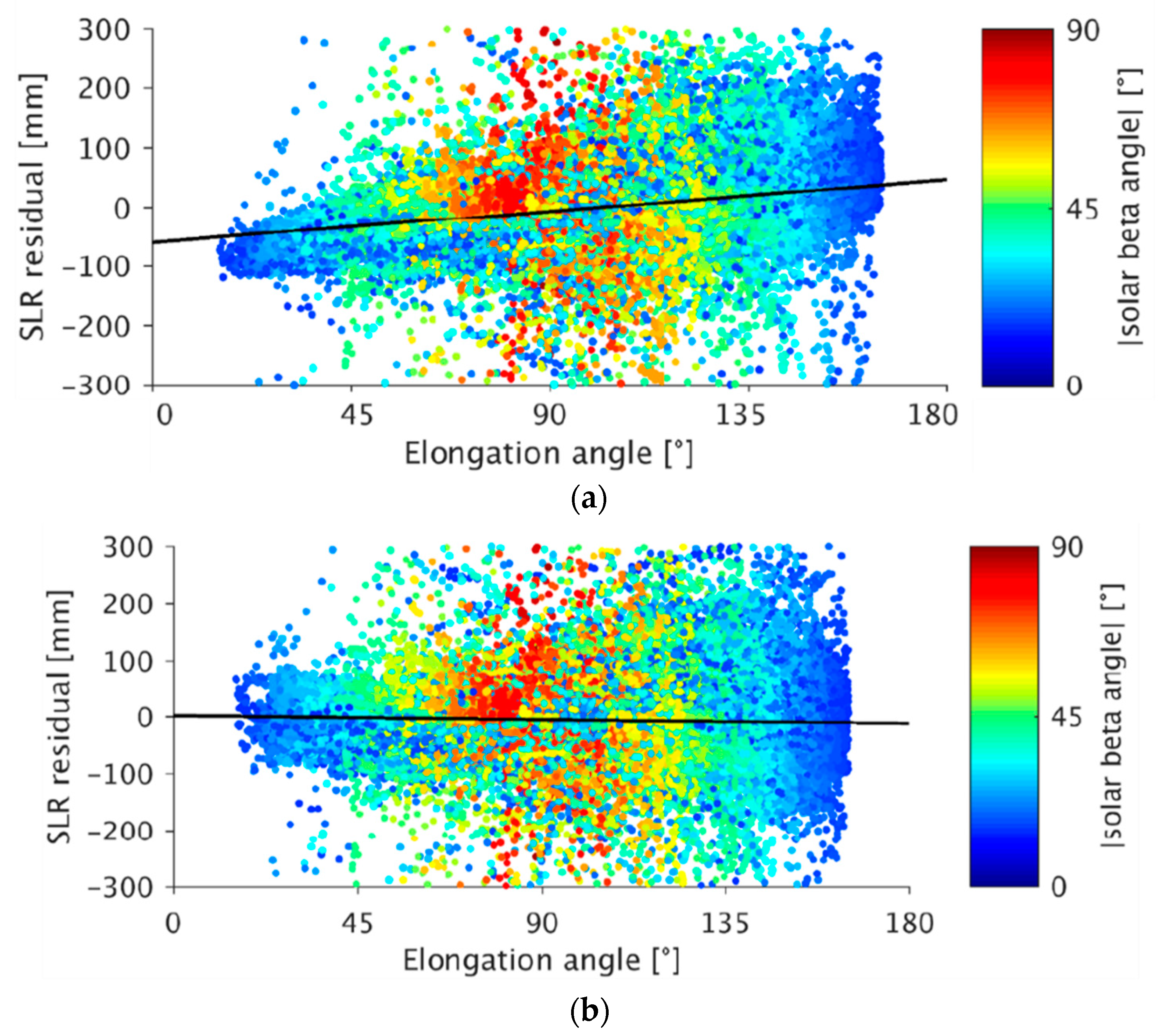
Figure 13 shows the SLR residuals of GLONASS-M orbits between January 2003 and December 2013. The systematic pattern, which can be seen for the orbits of IGS-repro02 (Figure 13, top), is significantly reduced when using the EGSIEM-REPRO orbits (Figure 13, bottom). This improvement is mainly related to the use of the extended ECOM instead of the original ECOM. The reasons for the larger scatter of the SLR residuals when using the extended ECOM (in particular for large elongation angles) are discussed in Section 4.
3.4. Quality Assessment Using GRACE Precise Orbit Determination
As a final quality control, GRACE POD based on undifferenced GPS data was performed to efficiently validate the global GPS orbit and clock solutions over all regions of the Earth by processing the data from a single receiver only.
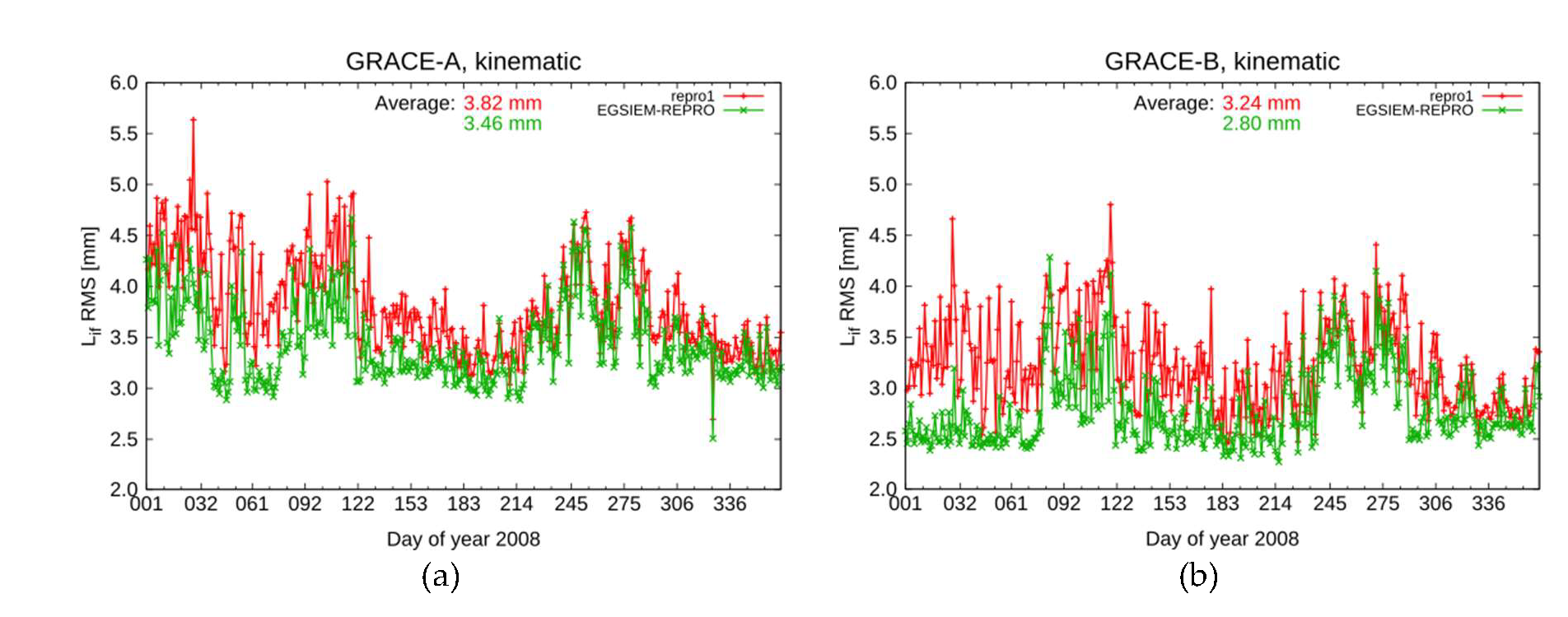
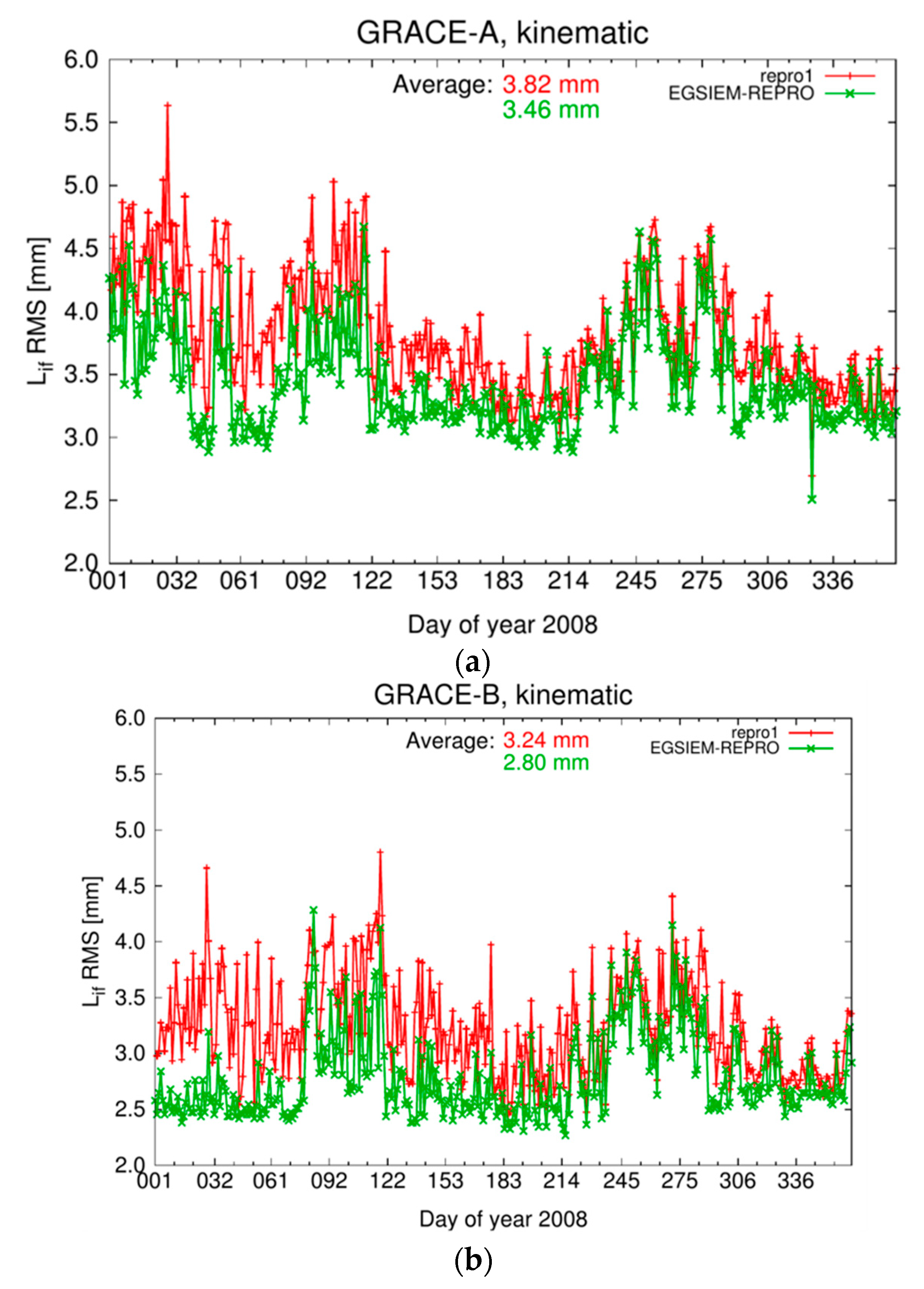
Figure 14 shows the daily RMS values of the ionosphere-free carrier-phase residuals of a kinematic orbit determination for GRACE-A (shown on left side of Figure 14) and GRACE-B (shown on the right side of Figure 14) over the year 2008. The values in red were calculated using the GPS orbits and clocks from CODE’s contribution to the first IGS reprocessing campaign (http://acc.igs.org/reprocess.html, henceforth repro1), while the values in green present the results obtained with EGSIEM-REPRO products. The reason why repro1 products were used for validation at this stage is that there is no consistent set of GPS orbits and clocks available from the CODE contribution to the IGS-repro02. More importantly, it was stated by [13] that the combined satellite clock corrections from different AC’s are severely limited by large residual biases and incompatible satellite attitude models adopted by different AC’s.
In both cases, the same antenna phase center variations were applied, which were estimated using EGSIEM-REPRO products. For most days, a clear reduction of the phase RMS can be seen, indicating a better fit of the GPS observations when using the new products. In terms of average values calculated over the entire year, the improvement for the GRACE-A and GRACE-B kinematic orbits is 0.36 and 0.44 mm, respectively.
Since the two GRACE satellites are equipped with SLR reflectors, we can make use of this technique as an independent orbit validation. For this analysis, normal points from 16 SLR stations (using coordinates from SLRF2008, which were extrapolated to epoch) were used. Laser reflector array (LRA) range corrections were applied according to [30]. Table 3 and Table 4 summarize the results of the SLR validation in terms of the mean and standard deviation values in mm for reduced-dynamic and kinematic orbits, respectively.
It can be seen that when using EGSIEM-REPRO, the SLR validation shows significantly better results compared to repro1 in terms of the standard deviation. For instance, the standard deviation of the SLR residuals for GRACE-B reduced-dynamic orbits is 4.37 mm smaller, which corresponds to a reduction of 25%.
4. Discussion and Outlook
According to [15], it is expected that the D4 term of the extended ECOM will be significantly smaller than the D2 terms. However, some cases were identified where the estimated solar radiation pressure parameters did not fit the expected behavior. For this reason, additional investigations were carried out.
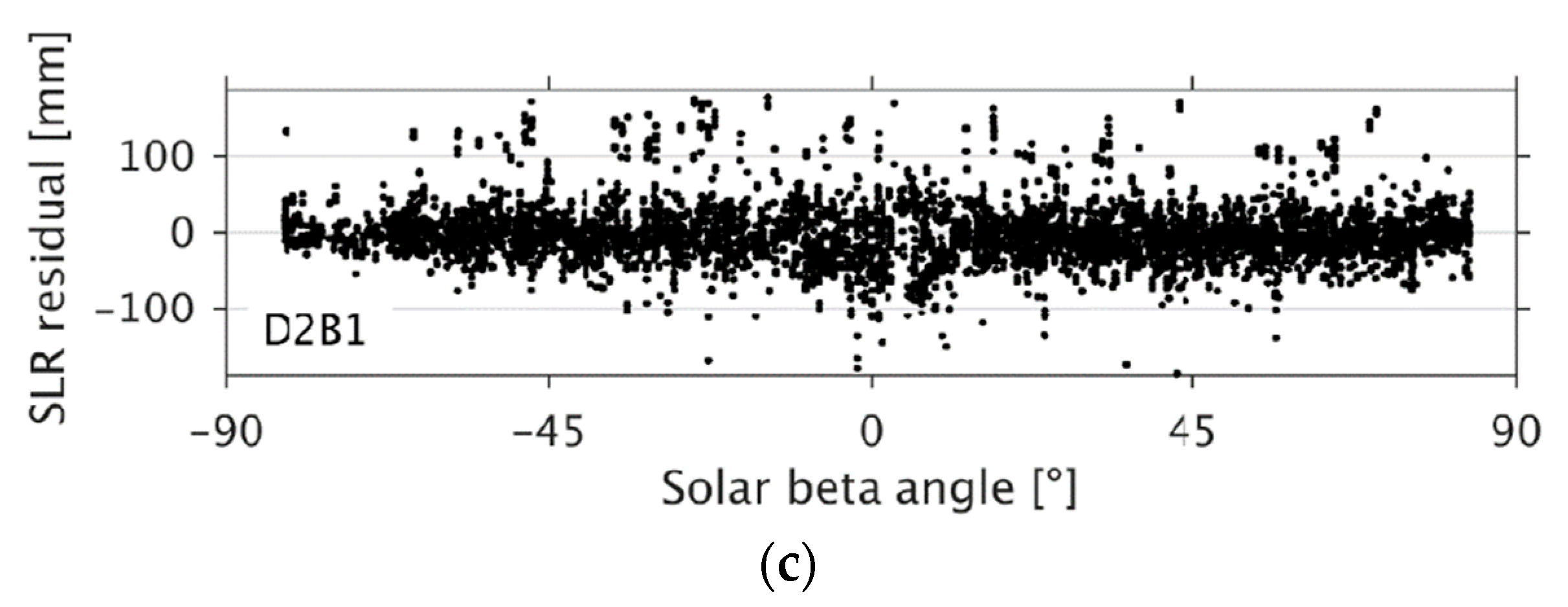
Figure 15 shows the SLR residuals of the orbits of the GLONASS satellite SVN 747, which were computed using three different types of empirical parametrization (see Table 1): D0B1, as used for IGS-repro02 (Figure 15a); D4B1, as used for EGSIEM-REPRO (Figure 15b); and D2B1 (Figure 15c).
In Figure 13, we show that by setting up 2-cpr and 4-cpr in the D direction, the systematic pattern of the SLR residuals with respect to the elongation angle of the Sun was significantly reduced. However, looking at the residuals as a function of the solar beta angle, we found degraded orbits whenever the solar beta angle was small. These periodic terms were used (Figure 15 b) rather than omitting them (Figure 15a). Setting up only the 2-cpr (and omitting the 4-cpr) parameter successfully decreased the residuals for small solar beta angles (Figure 15c) and preserved the advantage of a reduced systematic pattern with respect to the elongation angle. Table 5 presents the median and the interquartile range (IQR) of SLR residuals for GLONASS orbits between January 2012 and December 2014, computed using the three different types of parametrization.
In general, the median was closer to zero when estimating periodic terms in the satellite–Sun direction (solutions D4B1, D2B1). In addition, the IQR decreased by about 5 mm, indicating that the residuals were more centered on the median. Table 5 also highlights the abovementioned advantages of D2B1 parametrization over D4B1 parametrization—both the median and IQR are smallest for D2B1.
5. Conclusions
In the framework of the EGSIEM project, a dedicated reprocessing campaign was initiated, generating a full set of GNSS orbits, clock corrections, ERPs, troposphere parameters, and coordinate estimates, which are available at ftp://ftp.aiub.unibe.ch/REPRO_2015/.
During the reprocessing, several levels of quality control were established for the products and are presented in this paper. The GLONASS clock corrections were shown to be almost 100% complete. The reason for the periods with incomplete clock corrections may be attributed to incomplete RINEX data and limited available GLONASS tracking data. In terms of the stability of the generated GNSS satellite clock corrections, it has been shown that they are on the same level as operational CODE products. In particular, it has been shown that the densification of GLONASS satellite clock corrections from 300 to 30 s and then further to 5 s produced good results. Furthermore, using 5 s GNSS satellite clock corrections in terrestrial PPP analysis did not degrade the solution, but even improved it in some cases.
The validation of the GPS orbits and clock products by GRACE POD showed a clear reduction of the phase RMS value when using EGSIEM-REPRO products (about 13% for GRACE-A and 20% for GRACE-B) compared to repro1. The validation of the GNSS orbits using SLR data showed that the dependency of the SLR residuals on the elongation angle is significantly reduced when using EGSIEM-REPRO products.
However, some cases were identified where the theoretical assumption that the D4 terms of the extended ECOM are significantly smaller than D2 terms did not agree with the estimated solar radiation pressure parameters. Additional investigations showed the advantages of D2B1 over D4B1 parametrization—both the median and IQR of the SLR residuals were smaller for D2B1 by about 0.2 mm and 0.5 mm, respectively. Based on the lessons learnt from the EGSIEM-REPRO, the contribution from CODE to ongoing IGS reprocessing is based on the use of D2B1 parametrization.
Author Contributions
A.S. and R.D. designed the research; A.S. performed the research and wrote the paper; A.S., D.A., A.G., and G.B. analyzed the data; A.G., A.V., R.D., and G.B. contributed to the data analysis; A.V., R.D., D.A., A.G., G.B., and A.J. gave helpful suggestions during the internal reviewing process. All authors have read and agreed to the published version of the manuscript.
Funding
This research was funded by the European Union‘s Horizon 2020 research and innovation program under the grant agreement no. 637010 and the Swiss State Secretariat for Education, Research, and Innovation. All views expressed are those of the authors and not of the agency.
Acknowledgments
Authors would like to thank the International GNSS Service (IGS) for providing GNSS data used within the framework of this manuscript. Calculations were performed on UBELIX (http://www.id.unibe.ch/hpc), the HPC cluster at the University of Bern, Switzerland.
Conflicts of Interest
The authors declare no conflict of interest.
References
- Jäggi, A.; Weigelt, M.; Flechtner, F.; Güntner, A.; Mayer-Gürr, T.; Martinis, S.; Bruinsma, S.; Flury, J.; Bourgogne, S.; Steffen, H.; et al. European Gravity Service for Improved Emergency Management (EGSIEM)-from concept to implementation. Geophys. J. Int. 2019, 218, 1572–1590. [Google Scholar] [CrossRef]
- Tapley, B.; Bettadpur, S.; Ries, J.; Watkins, M. GRACE measurements of mass variability in the Earth system. Science 2004, 305, 503–505. [Google Scholar] [CrossRef] [Green Version]
- Jean, Y.; Meyer, U.; Jäggi, A. Combination of GRACE monthly gravity field solutions from different processing strategies. J. Geod. 2018, 92, 1313–1328. [Google Scholar] [CrossRef] [Green Version]
- Meyer, U.; Jean, Y.; Kvas, A.; Dahle, C.; Lemoine, J.-M.; Jäggi, A. Combination of GRACE monthly gravity fields on the normal equation level. J. Geod. 2019, 93, 1645–1658. [Google Scholar] [CrossRef] [Green Version]
- Zumberge, J.F.; Heflin, M.B.; Jefferson, D.C.; Watkins, M.M.; Webb, F.H. Precise point positioning for the efficient and robust analysis of GPS data from large networks. J. Geo. Res. 1997, 102, 5005–5017. [Google Scholar] [CrossRef] [Green Version]
- Dach, R.; Schaer, S.; Arnold, D.; Orliac, E.; Prange, L.; Sušnik, A.; Villiger, A.; Jäggi, A.; Beutler, G.; Brockmann, E.; et al. Center of Orbit Determination in Europe: IGS Technical Report 2017. In International GNSS Service: Technical Report 2017; Villiger, A., Dach, R., Eds.; (AIUB), IGS Central Bureau and University of Bern, Bern Open Publishing: Bern, Switzerland, 2018; pp. 32–44. [Google Scholar]
- Bock, H.; Beutler, G.; Schaer, S.; Springer, T.A.; Rothacher, M. Processing aspects related to permanent GPS arrays. Earth Planets Space 2000, 52, 657–662. [Google Scholar] [CrossRef] [Green Version]
- Bock, H.; Dach, R.; Jäggi, A.; Beutler, G. High-rate GPS clock corrections from CODE: Support of 1 Hz applications. J. Geod. 2009, 83, 1083–1094. [Google Scholar] [CrossRef] [Green Version]
- Beutler, G.; Rothacher, M.; Schaer, S.; Springer, T.A.; Kouba, J.; Neilan, R.E. The international GPS service (IGS): An interdisciplinary service in support of Earth sciences. Adv. Space Res. 1999, 23, 631–653. [Google Scholar] [CrossRef]
- Dow, J.; Neilan, R.; Rizos, C. The International GNSS service in a changing landscape of Global Navigational Satellite Systems. J. Geod. 2009, 82, 191–198. [Google Scholar] [CrossRef]
- Steigenberger, P.; Hugentobler, U.; Lutz, S.; Dach, R. CODE Contribution to the first IGS Reprocessing Campaign. Tech. Rep. 2011. 1/2011. Available online: http://www.bernese.unibe.ch/publist/2011/artproc/CODE_Repro1.pdf (accessed on 25 May 2020).
- Fritsche, M.; Sosnica, K.; Rodriguez-Solano, C.; Steigenberger, P.; Dietrich, R.; Dach, R.; Wang, K.; Hugentobler, U.; Rothacher, M. Homogeneous reprocessing of GPS, GLONASS and SLR observations. J. Geod. 2014, 88, 625–642. [Google Scholar] [CrossRef]
- Griffiths, J. Combined orbits and clocks from IGS 2nd reprocessing. J. Geod. 2018, 93, 177–195. [Google Scholar] [CrossRef] [PubMed] [Green Version]
- Altamimi, Z.; Rebischung, P.; Metivier, L.; Collilieux, X. ITRF2014: A new release of the International Terrestrial Reference Frame modeling nonlinear station motions. J. Geophys. Res. Solid Earth 2016, 121, 6109–6131. [Google Scholar] [CrossRef] [Green Version]
- Arnold, D.; Meindl, M.; Beutler, G.; Dach, R.; Schaer, S.; Lutz, S.; Prange, L.; Sosnica, K.; Mervart, L.; Jäggi, A. CODE’s new solar radiation pressure model for GNSS orbit determination. J. Geod. 2015, 89, 775–791. [Google Scholar] [CrossRef] [Green Version]
- Rebischung, P.; Griffiths, J.; Ray, J.; Schmid, R.; Collilieux, X.; Garayt, B. IGS08: The IGS realization of ITRF2008. GPS Solut. 2012, 16, 483–494. [Google Scholar] [CrossRef]
- Schmid, R.; Dach, R.; Collilieux, X.; Jäggi, A.; Schmitz, M.; Dilssner, F. Absolute IGS antenna phase center model igs08.atx: Status and potential improvements. J. Geod. 2016, 90, 343–364. [Google Scholar] [CrossRef] [Green Version]
- Dach, R.; Lutz, S.; Walser, P.; Fridez, P. (Eds.) The Bernese GNSS Software Version 5.2. User Manual; Astronomical Institute, University of Bern, Bern Open Publishing: Bern, Switzerland, 2015. [Google Scholar]
- The IGSMail Archives. Available online: https://lists.igs.org/pipermail/igsmail/2015/000869.html (accessed on 25 May 2020).
- Mervart, L.; Beutler, G.; Rothacher, M. Ambiguity resolution strategies using the results of the International GPS Geodynamics Service (IGS). Bull. Géodésique 1994, 68, 29–38. [Google Scholar] [CrossRef]
- Dach, R.; Schaer, S.; Lutz, S.; Meindl, A.; Bock, H.; Orliac, E.; Prange, L.; Thaller, D.; Mervart, L.; Jäggi, A.; et al. Center for Orbit Determination in Europe. IGS Technical Report 2011. In International GNSS Service: Technical Report 2011; Dach, R., Yean, Y., Eds.; IGS Central Bureau and University of Bern, Bern Open Publishing: Bern, Switzerland, 2012; pp. 21–34. [Google Scholar]
- Beutler, G.; Brockmann, E.; Hugentobler, U.; Mervart, L.; Rothacher, M.; Weber, R. Combining consecutive short arcs into long arcs for precise and efficient GPS orbit determination. J. Geod. 1996, 70, 287–299. [Google Scholar] [CrossRef]
- Caissy, M.; Agrotis, L.; Weber, G.; Hermandez-Pajares, M.; Hugentobler, U. The International GNSS Real-Time Service. GPS World 2012, 23, 52–58. [Google Scholar]
- Gurtner, W. RINEX: The receiver-independent exchange format. GPS World 1994, 5, 48–52. Available online: ftp://igs.org/pub/data/format/rinex2.txt (accessed on 15 May 2020).
- Lutz, S.; Meindl, M.; Steigenberger, P.; Beutler, G.; Sosnica, K.; Schaer, S.; Dach, R.; Arnold, D.; Thaller, D.; Jäggi, A. Impact of the arc length on GNSS analysis results. J. Geod. 2015, 90, 365–378. [Google Scholar] [CrossRef]
- Allan, D. Time and Frequency (Time-Domain) Characterization, Estimation, and Prediction of Precision Clocks and Oscillators. IEEE Trans. Ultrason. Ferroelectr. 1987, 34, 647–654. [Google Scholar] [CrossRef] [PubMed]
- Sosnica, K.; Thaller, D.; Dach, R.; Steigenberger, P.; Beutler, G.; Arnold, D.; Jäggi, A. Satellite laser ranging to GPS and GLONASS. J. Geod. 2015, 89, 725–743. [Google Scholar] [CrossRef] [Green Version]
- Rodriguez-Solano, C.; Hugentobler, U.; Steigenberger, P.; Blossfeld, M.; Fritsche, M. Reducing the draconitic errors in GNSS geodetic products. J. Geod. 2014, 88, 559–574. [Google Scholar] [CrossRef]
- Grahsl, A.; Sušnik, A.; Prange, L.; Arnold, D.; Dach, R.; Jäggi, A. GNSS orbit validation activites at the Astronomical Institute in Bern. In International Laser Ranging Service, Workshop 2016, 9–14 October 2016; Potsdam, Germany. Available online: https://cddis.nasa.gov/lw20/docs/2016/papers/P15-Maier_paper.pdf (accessed on 10 July 2020).
- Neubert, R.; Grunwaldt, L.; Neubert, J. The retroreflector for the CHAMP satellite: Final design and realization. In Proceedings of the 11th International Workshop on Laser Ranging, Deggendorf, Germany, 12–25 September 1998; pp. 260–270. [Google Scholar]
Figure 1.
Success rate of the ambiguity resolution for Globalnaya Navigatsionnaya Sputnikovaya Sistema (GLONASS) (blue color) and Global Positioning System (GPS) (red color) observations for the period 2000–2015.
Figure 1.
Success rate of the ambiguity resolution for Globalnaya Navigatsionnaya Sputnikovaya Sistema (GLONASS) (blue color) and Global Positioning System (GPS) (red color) observations for the period 2000–2015.

Figure 2.
Number of stations delivering high-rate Receiver Independent Exchange Format (RINEX2) data for the period 2003–2015.
Figure 2.
Number of stations delivering high-rate Receiver Independent Exchange Format (RINEX2) data for the period 2003–2015.

Figure 3.
Geographical distribution of stations providing high-rate RINEX2 data on January 1, 2003 (black dots), and on January 1, 2014 (red stars).
Figure 3.
Geographical distribution of stations providing high-rate RINEX2 data on January 1, 2003 (black dots), and on January 1, 2014 (red stars).

Figure 4.
(a) Time series of polar motion misclosures referring to the 2nd IGS reprocessing campaign (IGS-repro02). (b) Time series of polar misclosures referring to the reprocessing campaign carried out in the frame of the EGSIEM project (EGSIEM-REPRO). The top shows misclosures in the x coordinates and the bottom shows misclosures in the y coordinates, plotted with a shift along the vertical axis for clarity. Polar motion misclosures referring to the 1-day solution are shown with red, while polar motion misclosures referring to the 3-day solution are presented in blue.

Figure 5.
(a) Power spectrum of polar motion misclosures referring to the 2nd IGS reprocessing campaign (IGS-repro02). (b) Power spectrum of polar misclosures referring to the reprocessing campaign carried out in the frame of the EGSIEM project (EGSIEM-REPRO). Misclosures in x coordinates are shown on the top and misclosures in the y coordinates are shown on the bottom, plotted with a shift along the vertical axis for clarity. Polar motion misclosures referring to the 1-day solution are shown in red, while polar motion misclosures referring to the 3-day solution are presented in blue. In both cases, the chosen time interval is 2000–2014.

Figure 6.
(a) Power spectrum of polar motion misclosures for the 3-day solution referring to IGS-repro02. (b) Power motion of polar misclosures for the 3-day solution referring to EGSIEM-REPRO. The x coordinates are shown on the top and y coordinates are shown on the bottom. In both cases, the chosen time interval is 2000–2013.

Figure 7.
(a) The completeness of 30 s GLONASS (where each GLONASS satellite is shown with their pseudorandom noise numbers (PRN) number on the y axis) satellite clock corrections. (b) The completeness of 5 s GLONASS (where each GLONASS satellite is shown with their pseudorandom noise numbers (PRN) number on the y axis) satellite clock corrections. Note that the 5 s GLONASS clock corrections are only available from the end of 2010 onwards.

Figure 8.
(a) Allan deviations for satellites with space vehicle number (SVN) R747, G063, and G036 satellite clock corrections with different sampling corrections. (b) Allan deviations for satellites with space vehicle number (SVN) R724, G063, and G036 satellite clock corrections with different samplings. Both figures refer to October 27, 2013.

Figure 9.
(a) Root-Mean-Square (RMS) of the linear fit for selected GNSS satellite clock corrections shown in Figure 8a. (b) Root-Mean-Square (RMS) of the linear fit for selected GNSS satellite clock corrections shown in Figure 8b.

Figure 10.
(a) RMS in mm of the kinematic coordinates in the up (top), north (middle), and east (bottom) components for WTZR (Wettzell, Germany) station. (b) RMS in mm of the kinematic coordinates in the up (top), north (middle), and east (bottom) components for KIRU (Kiruna, Sweden) station. For both stations, the selected period is from December 11, 2013, to December 17, 2013.

Figure 11.
(a) Estimated kinematic coordinates in the north for two different sampling types, referring to the GPS+GLONASS solution. (b) Estimated kinematic coordinates in the north for two different sampling types, referring to the GPS solution. (c) Estimated kinematic coordinates in the north for two different sampling types, referring to the GLONASS solution. All three solutions refer to the first hour on December 17, 2013.

Figure 12.
(a) Allan deviations of estimated kinematic coordinates in the east component for two different samplings using GLONASS (indicated with GLO) only observations and satellite clock corrections. (b) Allan deviations of estimated kinematic coordinates in the north component for two different samplings using GLONASS only observations and satellite clock corrections. (c) Allan deviations of estimated kinematic coordinates in the up component for two different samplings using GLONASS only observations and satellite clock corrections. In all three figures, the Allan deviations were calculated over the entire day.

Figure 13.
(a) SLR residuals to GLONASS-M orbits from IGS-repro02 using the original Empirical CODE Orbit Model (ECOM). (b) SLR residuals to GLONASS-M orbits from EGSIEM-REPRO using the extended ECOM. For both figures, residuals between January 2003 and December 2013 are shown. Observations for four GLONASS satellites (space vehicle number (SVN) 723, 725, 736, 737) were excluded due to anomalous patterns. Residuals of these GLONASS satellites increased after a certain time after launch [29]. Furthermore, residuals with absolute beta angles smaller than 15◦ are not shown due to unmodeled attitude behavior during eclipses. The black line indicates the linear regression of the SLR residuals as a function of the elongation angle.

Figure 14.
(a) RMS of ionosphere-free carrier-phase residuals of kinematic precise orbit determination (POD) for GRACE-A. (b) RMS of ionosphere-free carrier-phase residuals of kinematic precise orbit determination (POD) for GRACE-B. The numbers indicate the average RMS values over the entire year. In both figures values in red were calculated using the GPS orbits and clocks from CODE’s contribution to the first IGS reprocessing campaign (repro1), while the values in green present the results obtained with EGSIEM-REPRO products.

Figure 15.
(a) SLR residuals as a function of the solar beta angle with respect to microwave-based orbits of GLONASS satellite SVN 747 over a three-year time span (January 2012 to December 2014): computed using the D0B1 parametrization of the ECOM model; (b) computed using the D4B1 parametrization of the ECOM model; (c) computed using D2B1 parametrization of the ECOM model.


Table 1.
Estimated empirical parameters in satellite–Sun direction (D), direction along the satellite’s solar panels axis (Y), and completion of the orthogonal right-handed system (B) for the original Empirical CODE Orbit Model (ECOM) and the extended Empirical CODE Orbit Model (ECOM2). Cycles-per-revolution is denoted as cpr.
| Empirical CODE Orbit Model (ECOM) | D | Y | B |
|---|---|---|---|
| D0B1 | constant | constant | constant, 1-cpr |
| D2B1 | constant, 2-cpr | constant | constant, 1-cpr |
| D4B1 | constant, 2-cpr, 4-cpr | constant | constant, 1-cpr |
Table 2.
Root-Mean-Squared (RMS) values of polar motion misclosures for the interval 2000–2014, resulting in IGS-repro02 (indicated with R-02 in the Table) and EGSIEM-REPRO (indicated with R-15 in the Table) in the x and y coordinates of the poles for the 1- and 3-day solutions, referring to different period intervals in microarcsecond (μas).
| Solution | Periods (Days) | X | Y | ||
|---|---|---|---|---|---|
| R-02 | R-15 | R-02 | R-15 | ||
| 1-day | All | 194.2 | 174.9 | 255.7 | 240.2 |
| <30 | 138.1 | 137.2 | 173.7 | 183.8 | |
| 30 < P < 600 | 135.5 | 106.9 | 182.2 | 153.1 | |
| 3-day | All | 28.7 | 29.5 | 29.9 | 29.6 |
| <30 | 26.9 | 28 | 28.3 | 28.7 | |
| 30 < P < 600 | 9.1 | 8.1 | 9.0 | 7.1 | |
Table 3.
Mean and standard deviation in mm of Satellite Laser Ranging (SLR) residuals for reduced-dynamic orbits over the entire year 2008. The number of used normal points in the analysis is given in brackets.
Table 3.
Mean and standard deviation in mm of Satellite Laser Ranging (SLR) residuals for reduced-dynamic orbits over the entire year 2008. The number of used normal points in the analysis is given in brackets.
| Product Identifier | GRACE-A | GRACE-B |
|---|---|---|
| repro1 | 1.99 ± 18.14 (32,587) | 0.09 ± 18.51 (31,008) |
| EGSIEM-REPRO | 2.21 ± 12.93 (32,639) | 0.70 ± 14.14 (31,030) |
Table 4.
Mean and standard deviation in mm of Satellite Laser Ranging (SLR) residuals of kinematic orbits over the entire year 2008. The number of used normal points in the analysis is given in brackets.
Table 4.
Mean and standard deviation in mm of Satellite Laser Ranging (SLR) residuals of kinematic orbits over the entire year 2008. The number of used normal points in the analysis is given in brackets.
| Product Identifier | GRACE-A | GRACE-B |
|---|---|---|
| repro1 | 1.24 ± 19.98 (32,358) | 0.44 ± 23.00 (30,343) |
| EGSIEM-REPRO | 2.11 ± 17.00 (32,409) | 1.24 ± 19.75 (30,456) |
Table 5.
Median and interquartile range (IQR) of SLR residuals with respect to GLONASS orbits between January 2012 and December 2014. The orbits were computed using three different orbit parametrizations, namely D0B1, D4B1, and D2B1. The observations for eclipsing satellites (absolute value of solar beta angle smaller than 15°) and for SVN 721, 723, 725, 730, 736, and 737 satellites were excluded due to anomalous patterns [15,29].
| Solution | Median (mm) | IQR (mm) |
|---|---|---|
| D0B1 | 5.0 | 38.0 |
| D2B1 | −2.4 | 32.8 |
| D4B1 | −2.6 | 33.3 |
© 2020 by the authors. Licensee MDPI, Basel, Switzerland. This article is an open access article distributed under the terms and conditions of the Creative Commons Attribution (CC BY) license (http://creativecommons.org/licenses/by/4.0/).
Share and Cite
MDPI and ACS Style
Sušnik, A.; Grahsl, A.; Arnold, D.; Villiger, A.; Dach, R.; Beutler, G.; Jäggi, A. Validation of the EGSIEM-REPRO GNSS Orbits and Satellite Clock Corrections. Remote Sens. 2020, 12, 2322. https://doi.org/10.3390/rs12142322
AMA Style
Sušnik A, Grahsl A, Arnold D, Villiger A, Dach R, Beutler G, Jäggi A. Validation of the EGSIEM-REPRO GNSS Orbits and Satellite Clock Corrections. Remote Sensing. 2020; 12(14):2322. https://doi.org/10.3390/rs12142322
Chicago/Turabian StyleSušnik, Andreja, Andrea Grahsl, Daniel Arnold, Arturo Villiger, Rolf Dach, Gerhard Beutler, and Adrian Jäggi. 2020. "Validation of the EGSIEM-REPRO GNSS Orbits and Satellite Clock Corrections" Remote Sensing 12, no. 14: 2322. https://doi.org/10.3390/rs12142322
Note that from the first issue of 2016, this journal uses article numbers instead of page numbers. See further details here.