Soil Moisture Estimate Uncertainties from the Effect of Soil Texture on Dielectric Semiempirical Models


State Key Laboratory of Remote Sensing Science, Aerospace Information Research Institute, Chinese Academy of Sciences, Beijing 100101, China
*
Author to whom correspondence should be addressed.
Remote Sens. 2020, 12(14), 2343; https://doi.org/10.3390/rs12142343
Submission received: 5 June 2020
/
Revised: 13 July 2020
/
Accepted: 16 July 2020
/
Published: 21 July 2020
Abstract
:Soil texture has been shown to affect the dielectric behavior of soil over the entire frequency range. Three universally employed dielectric semiempirical models (SEMs), the Dobson model, the Wang–Schmugge model and the Mironov model, as well as a new improved SEM known as the soil semi-empirical mineralogy-related-to-water dielectric model (SSMDM), incorporate a significant soil texture effect in different ways. In this paper, soil moisture estimate uncertainties from the effect of soil texture on these four SEMs are systematically and widely investigated over all soil texture cases at different frequencies between 1.4 and 18 GHz for volumetric water content levels between 0.0 and 0.4 m3/m3 from the perspective of two aspects: soil dielectric model discordance and soil texture discordance. Firstly, the effect of soil texture on these four dielectric SEMs is analyzed. Then, soil moisture estimate uncertainties due to the effect of soil texture are carefully investigated. Finally, the applicability of these SEMs is discussed, which can supply references for their choice. The results show that soil moisture estimate uncertainties are small and satisfy the 4% volumetric water content retrieval requirement in some cases. However, in other cases, it may contribute relatively significant uncertainties to soil moisture estimates and correspond to a difference that exceeds the 4% volumetric water content requirement, with potential for the largest deviations to exceed 0.22 m3/m3.
1. Introduction
The relationship between soil dielectric behavior and soil water characteristics is an essential part of a soil moisture estimate algorithm in microwave remote sensing. Uncertainties in these relationships will lead to uncertainties in the soil moisture estimations when these relationships are used to describe soil dielectric behavior as a function of only water content [1,2]. The complex dielectric permittivity of moist soil shows a strong dependence on the soil texture [3,4,5], and the complex dielectric permittivity measurements obtained from moist soil samples show that soil texture affects the dielectric behavior over the entire frequency range and is the most pronounced at frequencies lower than 5 GHz [6]. Soil texture is a stable, natural soil property that is widely used to characterize the physical properties of soil. Currently, the most widely used soil texture classification system in radiophysical and soil dielectric property studies is the classification of the United States Department of Agriculture (USDA) [7,8,9,10,11,12]. According to this classification, the following granulometric fractions are distinguished: sand particles have diameters of 0.2 cm > d > 0.005 cm; silt particles have diameters of 0.0002 cm < d < 0.005 cm; clay particles have diameters of d < 0.0002 cm; and the gravimetric weights of these particles are expressed in soil percentage. Clay particles mainly composed of crystalline minerals are the products of chemical weathering and generally flaky or needle-like and have a large specific surface area. Sand particles, which are generally spherical and have small specific surface areas, are typically composed of quartz, but may also include fragments of feldspar, mica, and heavy minerals. The mineral composition and physical properties of silt particles are generally similar to those of sand particles, but because of the smaller size and larger specific surface area per unit mass, silt particles are heavily coated by clay particles. Therefore, some of the physical and chemical properties of silt particles may be consistent with those of clay particles to some extent. Sandy soils are not as susceptible to various physicochemical processes as clay soils, resulting in a lower salinity of the soil water mixture in the case of sand [13]. The moist soil has different conductivity in dielectric properties resulting from the different contents of soluble salts and cation exchange capacities in relation to the specific surface area of soil particles. Additionally, soil texture is a key factor that controls the transitional volumetric water content threshold, which is used to distinguish bound water from bulk water, where coarse soil textures have lower values and fine textures have higher values [7,8,9,10,11,12,14]. Some studies have revealed that the Debye relaxation parameters (i.e., static dielectric constant, relaxation time, and effective conductivity) of the Debye relaxation formula in relation to soil texture can be employed to describe free soil water (FSW, i.e., free water in soil), which is different from liquid water (i.e., free out-of-soil water (FOSW)) [8,9,10,14].
Soil dielectric semiempirical models (SEMs), which include information on the physical background of dielectric behavior [7,8,9,10,11,12,14], are powerful and useful hybrids of empirical and physical models. SEMs have been widely employed in soil moisture estimates due to their ease of use with easily determined and readily available input parameters. However, soil dielectric SEMs are often calibrated for adjustable parameters with different measured complex dielectric permittivities over a specific set of soil samples. Thus, there may be some problems when they are applied to soil types that are not within the range of these soil types used to develop the relationship [14]. Currently, three widely used soil dielectric SEMs, the Wang–Schmugge model (referred to here as the Wang model) [12], the Dobson semiempirical model (referred to here as the Dobson model) [7,11], and the mineralogy-based soil dielectric model (MBSDM, also known as the Mironov semiempirical model and referred to here as the Mironov model) [9,10], have incorporated a significant soil texture effect. The Wang model was employed in the land parameter estimate model (LPRM algorithms) [15]. Many studies evaluating or improving the L-band Microwave Emission of the Biosphere model (L-MEB model) have considered the Dobson model [16,17] or the Wang model [18,19]. The Dobson model was adopted in the Aquarius Level-2 radiometer algorithm of the National Aeronautics and Space Administration (NASA) [20]. Furthermore, it was also chosen when the Soil Moisture and Ocean Salinity (SMOS) estimate scheme was defined. However, the Mironov model has been considered in SMOS soil moisture estimates in versions 5.5 and higher due to the model’s superior potential and performance compared with the Dobson and Wang models in some situations, as evidenced by the comparison with in situ L-band measurements [19,21,22,23]. The Wang, Dobson, and Mironov models were employed as alternative models in the soil moisture product of the Soil Moisture Active Passive (SMAP) mission [24]. Recently, a new improved SEM known as the soil semi-empirical mineralogy-related-to-water dielectric model (SSMDM) [14] was developed. To describe the Debye relaxation formula of FSW, the SSMDM considers the interaction between water and soil mineralogy) by correlating soil texture with the Debye relaxation parameters, rather than using the Debye relaxation spectrum of FOSW adopted in the Wang model. Additionally, the effective conductivity loss term related to both soil texture and soil moisture was introduced to explain the ionic conductivity losses of FSW.
Some effort has been devoted to the study of the difference among the Dobson, Wang, and Mironov models from the effect of soil texture. The soil moisture estimate uncertainties considering soil texture discordance with both the Wang and Dobson models were evaluated in [15]. However, only two textural cases were chosen: soil texture cases with 60% sand and 20% clay as well as with 20% sand and 60% clay. The results showed that considerable uncertainties exceed the 4% volumetric water content requirement at some volumetric water contents. In [25], Owe et al. compared the Wang and Dobson models at frequencies of 1.67 and 5 GHz with three soil texture casecases (forest soil with 57.4% sand and 10.5% clay; natural soil with 72.2% sand and 3.5% clay; and sandy soil with 92.7% sand and 0.6% clay) and found that the simulations agreed well with the laboratory measurements, except for the sandy soil. The results indicated that the use of the transitional moisture concept in the Wang model to clearly separate bound water from bulk water in the soil appears to align the model more closely with the laboratory measurements at low volumetric water contents. However, the simulations of the Dobson model are closer to the laboratory measurements at high volumetric water contents for natural and forest soil types. In order to select the appropriate model for the SMAP soil moisture estimation algorithm, P.K. Srivastava et al. [26] tested the simulation capability of different dielectric models applied to the soil texture case with approximately 62% sand and 14% clay at the L-band using data from a ComRAD ground-based SMAP simulator system. The analysis indicated that, although the temporal plots for retrieved soil moisture using the four dielectric models (the Mironov, the Dobson, the Wang, and the Hallikainen models) typically follow similar trends and that similar seasonal variations are observed between all the models and in situ datasets, the Mironov model was marginally better than the others for passive-only microwave soil moisture estimation in such situations. Laymon et al. [27] reported soil moisture estimates for the soil texture case with 8% sand and 21% clay at L- and S-bands using the Dobson model and the Wang model, and the obtained results were within 0.05 m3/m3. A comparison of the Dobson and Mironov models was performed in [22], which were employed in the L-MEB model for the SMOS soil moisture retrieval algorithm based on the SMOS level-1 brightness temperature observations. The research showed that the use of the Mironov model led to a higher estimate of soil moisture, with an average of 0.033 m3/m3 at a global scale, than the use of compared to the Dobson model. However, the discrepancy estimates were affected by uncertainties of the vegetation parameters, soil roughness etc. included in the L-MEB model. The results also showed that the comparisons of the two model outputs with in situ measurements at various test sites did not demonstrate a superior performance of one model over the other.
Nevertheless, most existing research is restricted to specific locations, limited soil types, and mainly low frequencies. Moreover, some comparisons among dielectric models from the effect of soil texture were based on the indirect relationship between soil moisture and microwave emissivity or backscattering, where uncertainties of the vegetation parameters, soil roughness etc. were introduced. The investigation of the direct relationship between soil dielectric property and soil moisture is a more effective means to evaluate the effect of soil texture on soil moisture estimates. Soil texture, as an important input of soil dielectric models, can vary significantly at the scale of a satellite-based radiometer footprint due to soil heterogeneity. This variation introduces another uncertainty source into the soil moisture estimates [15,28]. Therefore, questions relating to how soil texture affects these dielectric SEMs over all soil texture cases and the subsequent effects on the models’ soil moisture estimates represent urgent problems to be solved, examination of which can provide the basis for selection of the optimal soil dielectric model. The aim of this paper is to investigate systematically and widely the effect of soil texture on these four dielectric SEMs over all soil texture cases at different frequencies between 1.4 and 18 GHz for volumetric water content levels between 0.0 and 0.4 m3/m3. To quantitatively investigate how sand content, clay content, and silt content affect soil moisture estimates, a soil texture grouping according to the gravimetric weights of soil particles is developed to cover all soil texture cases. Soil moisture estimate uncertainties from the effects of soil texture on these four soil dielectric SEMs focus on two aspects: (1) from soil dielectric model discordance, which refers to the case in which one soil dielectric model is adopted during the input process and a different soil dielectric model with the same soil texture is adopted during the estimation process, leading to a deviation of soil moisture estimate result; and (2) from soil texture discordance, which refers to the case in which one soil texture case is adopted as the input of the dielectric model during the input process and a different soil texture case is adopted as the input of the same dielectric model during the estimation process, leading to a deviation of soil moisture estimate result. Furthermore, the applicability of these four SEMs over all soil texture cases is discussed. The investigation can provide a theoretical basis for the choice of dielectric models over all soil texture cases.
2. Materials and Methods
2.1. Model Descriptions
All these four SEMs are volumetric models that describe soil dielectric properties based on the relative volume amounts of different soil constituents and their individual dielectric characteristics. The exponential model, which is based on the Lichtenecker–Rother model, is one of the most popular volumetric models. This exponential model for a material with n components can be written as follows [29,30]:
where is the volume fraction of the ith substance constituent and the scaling factor is an empirical variable. gives the volumetric mixing models a semi-empirical nature. In general, is treated as a constant structural factor. However, A. Brovelli and G. Cassiani [31] suggested that the exponent depends on the volumetric water content or effective dielectric permittivity. Wagner et al., 2011, [29] proposed the so-called Advanced Lichtenecker and Rother Model (ALRM), which treats as a function of volumetric water content and soil porosity P.
All these four SEMs treat soil–water–air systems (i.e., moist soils), representing heterogeneous multiphase mixtures, as a four-phase system composed of dry soil, air, bound water, and bulk water. Equation (1) can be rewritten to Equation (2), and the models have different values; is set to 0.65 in the Dobson model, 0.5 in the Mironov model (i.e., a linear combination of the complex refractive index for every constituent), 1 in the SSMDM (i.e., linear combination of complex dielectric permittivity for every constituent), and both 1 and 0.5 in the Wang model.
with
where and are the volume fractions of bulk water and bound water, respectively. , , , and are the complex dielectric permittivities of bulk water, bound water, air, and solid particles, respectively. is the dry bulk density of soil. is the soil particle density. The dielectric property of is frequency independent in the considered temperature–pressure–frequency range in all of these four SEMs.
2.2. Soil Texture Grouping Over All Soil Texture Cases
To cover all soil texture cases to quantitatively investigate how sand content, clay content, and silt content affect soil moisture estimates, a soil texture grouping at 5% increments is developed based on soil texture proportions and the particle size class of the USDA classification standard. The soil texture grouping divides all soil texture cases into four sections: I: soil texture cases with clay contents greater than or equal to 50%; II: soil texture cases with sand contents greater than or equal to 50%; III: soil texture cases with silt contents greater than or equal to 50%; IV: other soil texture cases. The nodes of each soil type are located at 5% increments of the particle content (sand, silt, or clay contents) in the soil texture ternary diagram, and, in each partition, the nodes are labeled with letters from the English alphabet, as shown in Figure 1. All of the soil texture cases are used to further investigate the differences among the four SEMs and to assess the applicability of each model to each soil type.
2.3. Methods of Soil Moisture Estimate
To evaluate the effects of soil texture on soil moisture estimates due to soil dielectric model discordance, the simulations of the real parts of the complex dielectric permittivities by one model are used to construct a lookup table (LUT), and the simulations by another model are treated as the resultant dielectric constant measurements used to estimate the soil moisture content. Then, the differences between the input and retrieved soil moisture contents are analyzed. Firstly, the forward model parameters are optimized, and representative soil surface parameters are employed. These parameters include soil moisture levels between 0.0 and 0.4 m3/m3, a typical soil bulk density value, a room temperature value, and frequencies from 1.4 to 18 GHz. Secondly, all possible variable values from the first step are input into the forward model to calculate the complex dielectric permittivity databases to form an LUT. Thirdly, the soil moisture content is evaluated based on the LUT by identifying the values with the minimal errors compared to the resultant dielectric constant measurements via the minimized cost function. Finally, the corresponding input and retrieved soil moisture are extracted. Six different combinations are obtained as follows:
- 1:
- Mironov–Dobson
- 2:
- Wang–Dobson
- 3:
- SSMDM–Dobson
- 4:
- Mironov–Wang
- 5:
- SSMDM–Wang
- 6:
- Mironov–SSMDM
where, for example, ‘Mironov–Dobson’ indicates that the Dobson model simulation is used to construct the LUT and the Mironov model simulation is treated as the resultant dielectric constant measurements from which the soil moisture content is acquired. Other terms have similar meanings.
Moreover, the effects of soil texture on soil moisture estimates due to soil texture discordance are examined by introducing the wrong soil texture into the soil moisture estimate process. To evaluate the uncertainty arising from the soil moisture estimate with soil texture discordance under the same soil dielectric model, the simulations of the real part of the complex dielectric permittivities with one soil texture are used to construct an LUT, and the simulations with another soil texture are treated as the resultant dielectric constant measurements used to evaluate the soil moisture content. Three possible methods of soil texture changes with grain size content changes of 20%, 40%, 60%, and 80% are as follows:
- The soil texture changes from clay to silt, and the sand content remains constant: from ‘H’ (clay) to ‘H1’ (clay), from ‘H’ (clay) to ‘C1’ (loam), from ‘H’ (clay) to ‘E1’ (silt), and from ‘H’ (clay) to ‘I’ (silt).
- The soil texture changes from sand to silt, and the clay content remains constant: from ‘I’(sand) to ‘E1’ (sand), from ‘I’ (sand) to ‘A’ (loam), from ‘I’ (sand) to ‘H1’ (silt), and from ‘I’ (sand) to ‘H’ (silt).
- The soil texture changes from sand to clay, and the silt content remains constant: from ‘H’ (sand) to ‘H1’ (sand), from ‘H’ (sand) to ‘H’ (loam), from ‘H’ (sand) to ‘E1’ (clay), and from ‘H’ (sand) to ‘I’ (clay).
3. Results and Analysis
3.1. The Effect of Soil Texture on Models
3.1.1. Different Ways Considering Soil Texture
The four investigated models incorporate a significant soil texture effect in different ways. The differences are primarily reflected in these aspects: the distinction between bound water and bulk water, the dielectric properties of dry soil, the dielectric properties of bulk water, and the dielectric properties of bound water, especially for the conductivity losses included in the imaginary part of bulk water and of bound water. Moreover, the Wang, SSMDM, and Dobson models take both the clay percentage and the sand percentage as the input parameters of soil texture, whereas the Mironov model, with the clay percentage as the sole input parameter of soil texture.
- The distinction between bound water and bulk water
With the exception of the Dobson model, due to a lack of physical consideration of the dielectric properties of bound water, the Wang, SSMDM, and Mironov models use the maximum bound water fraction (MBWF, i.e., transition moisture), which is related to the soil texture, to clearly distinguish between bound water and bulk water. In the SSMDM or Wang model, the MBWF has a physical meaning since it is related to the soil wilting point by empirically fitting according to measurements, and the relationship between soil wilting point and soil texture has been empirically derived by Schmugge et al. from regression over 100 datasets of soil moisture characteristics [12] (Equations (5) and (6)). In the Mironov model, the MBWF is obtained through straight line fitting using measured complex refractive indexes (Equation (7)). The values of MBWF for these three models versus the clay fraction are shown in Figure 2. The results show that, although the clay fraction is also the key factor for MBWF in the SSMDM or Wang model, which is similar to that in the Mironov model, the discrepancy between them is obvious. The MBWF values in the Mironov model have a wider range versus the clay percentage and are lower than those in the SSMDM or Wang models. At low clay percentages, the values of the MBWF from the Mironov model are too low to agree with experiments, demonstrating that similar soils possess transition points varying between 0.19 and 0.24 in [13] and 0.26 in [18], which are closer to those from the Wang or SSMDM models. In the Dobson model, an empirical coefficient of exponent , which depends on soil texture, and the volumetric water content , including both bulk water and bound water, is introduced to determine the contributions of both bound water and bulk water as follows:
with
- The dielectric properties of dry soil
In the Wang, Dobson, and SSMDM models, the dielectric permittivities of dry soil where the volumetric water content is zero, there is a relationship described by Equation (8) because is 1., and , , are treated as an input to compute based on the theoretical formula ((2), (3), and (10)). The dielectric measurements for three of the most common clay minerals—kaolin, illite, and montmorillonite—indicate that the permittivity of these minerals is reasonably similar, between 5 and 6, and the measured permittivity of ground quartz is 4.4 [32]. Therefore, is not a constant. However, for simplicity, a constant is employed in the SSMDM, Dobson, and Wang models. Therefore, users can adjust it if necessary. In the Mironov model, the dielectric permittivity of dry soil is only related to the clay fraction by empirical fitting of the used experimental measurements, the detailed information has been described in [10]. Furthermore, increases with the clay fraction in the Wang, SSMDM, and Dobson models, which is in accordance with the measurements [32], and vice versa in the Mironov model, which may underestimate , especially when the clay fraction increases.
- The dielectric properties of bulk water
To account for the bulk water frequency dispersion, the Debye relaxation formula for FOSW is employed in the Wang model (Equation (9)) and Dobson model (Equations (10) and (11)). However, considering that the situation of bulk water in soil is different from that of the FOSW, the Debye relaxation formulae of the FSW are adopted in the SSMDM (Equations (12)–(15)) and Mironov models (Equations (16)–(19)) to correlate the dielectric spectroscopic parameters with soil texture. Conductivity loss plays an important role at low frequencies, and relaxation loss due to the dipolar relaxation of bulk water becomes important toward the high-frequency end [14]. In the Wang model, a conductivity loss () is added to the imaginary part of the bulk water complex dielectric permittivity at low frequencies, and is an empirical coefficient. In the Dobson model, the conductivity loss term depends on the volumetric water content, soil texture, soil bulk density, and particle density (third part of Equation (10)), and the effective conductivity () is an empirically derived function of soil texture and (Equation (11)). In the SSMDM, the effective conductivity loss term () is introduced, which is correlated with both soil texture and soil moisture, to account for the conductivity loss in the imaginary part, and different relationships at frequencies of 1.4–12 GHz and 12–18 GHz are adopted (Equation (15)). In the Mironov model, the FSW conductivity loss term is related to only the clay percentage (Equation (19)). Although both the SSMDM and the Mironov model consider bulk water as FSW by correlating the dielectric spectroscopic parameters with soil texture, they are different. In the Mironov model, and are constant, and R2 between and MBWF is 1 since both are empirically fitted linearly with the clay percentage. However, in the SSMDM, R2 between MBWF and is very low: 0.0068 (at 1.4–12 GHz) and 0.0763 (at 12–18 GHz).
where , , , and are the high-frequency limits of dielectric constant, the static dielectric constant, the relaxation time, and the effective conductivity of the out-of-soil water, respectively [33,34]; is the frequency in hertz; and is the permittivity of free space equal to 8.854 * 10−12 F·m−1. is not dependent on either temperature or salinity, and the parameter quantity is equal to 4.9 [8]:
with
with
or
where is the dielectric constant at the FSW high-frequency limit, which is assumed to be equal to [8]; and are the static dielectric constant and relaxation time of FSW, respectively; and is the FSW effective conductivity in S/m.
with
1.4 GHz ≤ f ≤ 12 GHz
f > 12 GHz
- The dielectric properties of bound water
In the Dobson model, the bound water dielectric property is not physically considered as described above. In the SSMDM and Wang models, both complex dielectric permittivities of ice and bulk water are utilized to determine the bound water complex dielectric permittivity (Equation (20)) via an adjustable weight factor (Equation (21) in the SSMDM and Equation (22) in the Wang model), and the former treats bulk water as FSW but the latter treats bulk water as FOSW. Furthermore, the bound water complex dielectric permittivity in both the Wang and SSMDM models changes with the soil volumetric water content when soil moisture is lower than the MBWF. The study of D. A. BoyarskiI et al. [18] also indicated that the complex dielectric permittivity of bound water depends on the thickness of the bound water film covering soil particles, and a change in the volume of bound water in soil leads to a change in its dielectric properties. However, in the Mironov model, it is assumed that the permittivity of the bound water is constant with the changing of the soil volumetric water content when soil moisture is lower than the MBWF. Moreover, bound water is treated as bound water in soil (i.e., bound soil water (BSW)) by correlating the dielectric spectroscopic parameters with the clay fraction through straight line fitting with the measured soil complex dielectric permittivities (Equations (24)–(26)), and also follows Debye’s formula (Equation (23)).
or
where is a parameter that can be chosen to best fit the experimental data with a nonlinear regression in the SSMDM. is related to in the Wang model.
with
where is the dielectric constant at BSW high-frequency limit, which is also assumed to be equal to ; , , and are the static dielectric constant, relaxation time, and the effective conductivity of BSW, respectively.
3.1.2. Simulation Differences and Reliability Evaluation
In this section, the simulations of these four models over all soil texture cases combing with some existing validations are employed to compare the difference among models and to evaluate the reliabilities of models because complex dielectric permittivity laboratory analyses performed by reproducing precise field conditions in laboratory soil samples are not easy and entirely straightforward. The soil texture cases of the existing validations are described in Table 1. However, some similar soil texture cases from these references are inconsistent with each other, probably because of the uncertainties from the measurements or some other factors that affect the dielectric properties of moist soil, such as between HARLINGEN CLAY and MILLER CLAY from [12], which leads to the difficulty of the validation.
Only some typical simulations of are shown in Figure 3 due to the high level of similarity for most soil texture cases. The simulated values of the Dobson model present a more linear trend versus soil moisture, and a maximum difference between the Dobson model and other models exists for soil texture cases in Sections II and IV at low and medium volumetric water contents due to the lack of distinction between bound water and bulk water, which has been validated by the measurements of the corresponding soil texture cases in [25] and the comparisons between the measurements and the simulations of these models in [14], and may also lead to a high level of uncertainty when it is used to predict the complex dielectric permittivities of soils that are outside the ensemble of prototypical soils used for model development, which also have been discussed in [22]. For soil texture cases in Section III, when the silt content is less than 60% or between 60% and 70% with a low sand content, which is also related to frequency, the values of these four models are relatively consistent, which has been validated by the measurements in [23], except when the clay content is at least 40%, the simulations of the Wang model are slightly lower at medium and high soil moisture. The differences among models cannot be neglected at medium and high moisture contents when the silt content is greater than approximately 75%, which increases with the sand content. For soil texture cases in Section II, when the silt content is greater than approximately 35% or between 30% and 35% with a low clay content, and for soil texture cases in Section IV with a clay content less than the silt content by 15% or more, the values of the four models are relatively consistent. The exception is the differences between the Dobson model and the other models at low moisture contents due to the lack of distinction between bound water and bulk water in the Dobson model, which has been validated by the corresponding soil texture cases of measurements in [7,25,26]. For soil texture cases in Section I, and other cases in Sections II and IV, the differences between the Dobson and the Wang and Mironov models cannot be neglected and the values of the SSMDM are consistent with those of the Wang and Mironov models at low moisture contents but approach the results of the Dobson model at high moisture contents. The Wang and Mironov models are comparably consistent with each other, except for soil texture cases in Section I with low sand contents, and for soil texture cases in Section III when the silt content is greater than 60% with high silt or sand contents at high frequencies.
Only some typical simulations of are shown in Figure 4. The effects of soil texture and frequency on are more complicated than those on . The simulations show that the values at low frequencies (such as at the L-band) are very different from those at high frequencies. At the L-band, when the sand content is at least 80% or at least 75% with clay contents less than approximately 5%, of the Wang model has negative values, and of the Dobson model has negative values when the sand content is at least 70% or the sand content is greater than the clay content by approximately 45% or more for soil texture cases in Section II. Therefore, for these cases it is not reasonable to describe the imaginary part of the complex dielectric permittivity.
At the L-band, for soil texture cases in Section II, the of the SSMDM are close to those of the Wang model when the sand content is less than approximately 60% with a low silt content, and the of the Mironov model are close to those of the Wang model when the sand content is less than 60% with a low clay content. For soil texture cases in Section I, the values of the SSMDM are close to those of the Wang model, especially for soil texture cases with high clay contents, and a small difference exists when the clay content decreases. The values among these four SEMs are obviously different at medium and high moisture contents for soil texture cases in Sections III and IV; however, when the silt content is at least 65% with a low clay content, the values of the Mironov and Dobson models are relatively consistent. At C-, X-, and Ku-bands, the values of the Mironov model are basically in agreement with those of the Wang model for soil texture cases in Sections II and IV and for soil texture cases in Section I when the clay content is less than approximately 55% with a low silt content. The values of the SSMDM, Mironov, and Wang models are basically consistent for soil texture cases in Section III when the silt content is less than 65% or between 65% and 70% with a low clay content and for soil texture cases in Section II when the silt content is at least 35%. The values of the Dobson model are basically consistent with those of the SSMDM for soil texture cases in Section II when the silt content is low at high frequencies and when the sand content is less than approximately 60% with a low silt content at low frequencies.
The simulations of the real parts for different soil texture cases by changing 20% of particle contents under the same model are depicted in Figure 5, under three different situations—keeping sand content constant, keeping clay content constant and keeping silt content constant—to display the soil texture sensitivities of the studied SEMs. The results show that the simulations of for the Wang and Mironov models are relatively consistent for many cases in Section III due to the similarity of their sensitivity to clay content and insensitivity to sand content, although the Wang model is theoretically very different from the Mironov model in the way soil texture is considered. The exception is that, in some cases, the soil moisture estimate deviations due to model discordance are larger than 0.04 m3/m3 at low moisture contents at low frequencies, or at low and medium moisture contents at high frequencies, due to the different treatments of the dielectric properties of solid particles and dry soil, as well as the MBWF, especially for samples with high clay contents at high frequencies. The Dobson model is highly sensitive to sand content but not clay content, which is very different from the Wang or Mironov models, and thus causes the largest soil moisture estimate deviations between the Dobson and Wang or Mironov models. The SSMDM is highly sensitive to sand content at high volumetric water contents, and both the sand and clay contents affect the model, especially at low and medium soil moisture.
3.2. Soil Moisture Estimate Uncertainties
3.2.1. Soil Moisture Estimate Uncertainties from Soil Dielectric Model Discordance
The deviations of soil moisture estimate results due to soil dielectric model discordance for some typical soil texture cases at different frequencies are depicted in Figure 6, and the deviations of six different model combinations compared to 0.04 m3/m3 have been described carefully in Table A1 from Appendix A. The results show that, in some cases, the deviations of soil moisture estimate results for these four dielectric models are relatively comparable and satisfy the 4% volumetric water content retrieval requirement. However, scenarios in which the content of sand or silt is very high, the content of clay is high, or the content of silt is low may contribute relatively significant uncertainties to soil moisture estimates that exceed the 4% volumetric water content requirement. The largest deviations, with a value of over 0.22 m3/m3, occur for the ‘A’ sample in Section I with 100% clay content due to the difference between the Dobson and Wang or Mironov models. The largest deviation for soil texture cases in Section II, with a value of 0.13 m3/m3, occurs for the ‘M2′ sample between the Wang and Dobson models at the Ku-band in the vicinity of 0.28 m3/m3. For soil texture cases in Section IV, the largest estimate deviation with a value of 0.12 m3/m3 occurs for the ‘J1′ sample between the Wang and Dobson models at L- or Ku-bands in the vicinity of 0.28 m3/m3. For soil texture cases in Section III, the largest estimate deviation, with a value of 0.11 m3/m3, occurs for the ‘A’ sample with 100% silt content between the Mironov and Dobson models at the Ku-band.
The estimate deviations are small and below 0.04 m3/m3 for all possible combinations of models when the silt content ranges from 55% to 70% with a relatively low sand content or ranges from 50% to 55% with a relatively low clay content for soil texture cases in Section III, when the silt content is greater than approximately 25% with a low clay content for soil texture cases in Section II, or when the silt content is greater than approximately 35% with a low clay content for soil texture cases in Section IV, except for some cases greater than 0.04 m3/m3 at medium water content induced by the difference between the Dobson and other models due to the lack of distinction between bound water and bulk water in the Dobson model for soil texture cases in Sections II and IV. The estimate deviations due to the difference between the Wang and Mironov models (‘4′) are generally small and less than 0.04 m3/m3, except for some cases with relatively high clay contents for low medium volumetric water contents at low frequencies, or for low and medium volumetric water contents at high frequencies. The estimate deviations due to the difference between the SSMDM and Dobson models (‘3′) are generally small and less than 0.04 m3/m3 when the silt content is greater than 40%, except for a few cases at medium moisture contents due to the lack of distinction between bound water and bulk water in the Dobson model and at high moisture contents for high frequencies when the silt content is ≥85%.
Generally, the estimate deviations due to the difference between the Dobson and another models (Mironov model (‘1′) or Wang model (‘2′)) are larger than for other combinations. When the clay content is greater than 55% for soil texture cases in Section I, or the silt content is less than 10% or ranges from 10% to 20% with a high clay content for soil texture cases in Section II, or when the clay content is greater than 35% with a low silt content for soil texture cases in Section IV, the estimate deviations of ‘1′ and ‘2′ are large and greater than 0.04 m3/m3 for all soil moisture levels between 0.0 and 0.4 m3/m3, except for rare cases at very low moisture levels. For soil texture cases in Section III, the estimate deviations of ‘1′ and ‘2′ are large and greater than 0.04 m3/m3 at medium and high volumetric water contents when the silt content is greater than approximately 70%.
3.2.2. Soil Moisture Estimate Uncertainties from Soil Texture Discordance
Based on the same soil texture cases discussed in Section 3.1.2, the deviations of soil moisture estimate results due to soil texture discordance are depicted in Figure 7. The results show that soil texture discordance has very little influence on soil moisture estimates and the deviations are always less than or close to 0.04 m3/m3 with the Dobson model when the sand content remains constant, even when the soil texture varies from ‘H’(I) to ‘I’(III); or with the Wang model when the clay content is constant, even when the soil texture varies from ‘I’(II) to ‘H’(III); or with the Mironov model when the clay content is constant, where the soil moisture estimate deviations are zero because only the clay content is employed. However, the deviations with the Dobson model are greater than 0.04 m3/m3 at medium and high volumetric water contents when the soil texture varies from ‘I’(II) to ‘E1′(II) with constant clay content, and the deviation reaches approximately 0.16 m3/m3 when the soil texture varies from ‘I’ (II) to ‘H’(III). The estimate deviations with the Wang or Mironov models are distinct because of the change in clay content, with values of approximately 0.18 and 0.20 m3/m3, respectively, when soil texture varies from ‘H’(I) to ‘I’(III). Both sand and clay contents affect the SSMDM at low volumetric water contents, whereas the sand content is more important at high volumetric water contents. When the soil texture varies from sand to clay with constant silt content, the deviations with the Mironov or Wang models, which are close to 0.04 m3/m3 when the soil texture changes from ‘H’(II) to ‘H1′(II), are larger than those with the SSMDM or Dobson models, and the largest value of greater than 0.20 m3/m3 occurs for the Wang model when the soil texture varies from ‘H’(II) to ‘I’(I). A 20% error in the sensitive soil components of the corresponding models will result in soil moisture estimate deviations greater than 0.04 m3/m3 except for the SSMDM. The deviations with the Wang or Mironov model are greater than 0.04 m3/m3 at medium and high volumetric water contents when a 20% clay content error with constant sand is introduced. The deviations with the Dobson model are greater than 0.04 m3/m3 at medium and high volumetric water contents with a 20% sand content error with constant clay content.
4. Discussion and Conclusions
The soil moisture estimate deviations introduced by soil texture discordance with constant silt content compared to those with constant sand content or clay content should be the largest since the physical and chemical properties of the silt particles lie between those of the clay particles and sand particles. However, because the Mironov model uses clay as the only soil texture input, the model cannot describe this characteristic exactly, and soil texture discordance with invariant clay contents shows that the deviations are the largest in the Dobson model. Therefore, a theoretical problem in explaining the influence of soil texture likely exists in the Dobson model. Although both soil texture discordance and soil dielectric model discordance may lead to soil moisture estimate deviations of greater than 0.20 m3/m3, soil texture discordance can produce larger uncertainties with large changes in the sensitive soil particle.
When the soil moisture is very low, such as volumetric water contents of ≤0.07 m3/m3, which is simply an estimated value according to the simulations over all soil texture cases, the Mironov model relates the clay content to the complex dielectric permittivity of dry soil, and may lead to an obvious underestimation when the clay content is large, and the Dobson model cannot accurately describe the complex dielectric permittivity of moist soil when the sand content or clay content is large due to the lack of distinction between bound water and bulk water. With the exception of situations in which the soil moisture is very low, from the theory, simulations and some existing validations of the influence of soil texture on these SEMs, combined with the results of soil moisture estimation uncertainties from soil texture discordance and soil dielectric model discordance, we have the following conclusions, which are references for the choice of soil dielectric models:
- For soil texture cases under the condition of 55% ≤ silt content ≤ 70% with low sand content, and 50% ≤ silt content ≤ 55%, the discrepancies between these four SEMs are small, and similar results can be achieved with all of them when chosen for soil moisture retrieval algorithms, except a few cases under the condition of 50% ≤ silt content ≤ 55% with high clay content (about >40%), where soil moisture estimation deviations are a little higher than 0.04 m3/m3 due to the discrepancies between the Dobson and Wang model at low soil moisture.
- For soil texture cases under the condition of silt content ≥ 15% with low clay content for soil texture cases in Section II, and silt content ≥ 20% with low clay content for soil texture cases in Section IV, with the exception of the Dobson model at low and medium volumetric water content due to the lack of distinction between bound water and bulk water, the discrepancies between the Wang, Mironov, and SSMDM models are small, and similar results are achieved.
- For soil texture cases under the condition of silt content ≥ 15% with high clay content for soil texture cases in Section II and silt content ≥ 20% with high clay content for soil texture cases in Section IV, the deviations will exceed the 4% volumetric water content requirement between the Dobson model and another model at low or medium water volumetric water content due to the lack of distinction between bound water and bulk water, and between the Wang and other models (i.e., Mironov or SSMDM model) at low water volumetric water content; whereas the discrepancies between the Mironov and SSMDM models are small. And these two SEMs for soil moisture retrieval algorithms can be considered firstly because both of them consider the dielectric properties of FSW. However, these soil texture cases lack validation with experimental data, and more accurate experimental data are needed to assess them.
- The Mironov model, in which the clay percentage is the sole input parameter of soil texture, may introduce some uncertainties for soil texture cases with a large proportion of a certain component. For soil texture cases under the condition of 55% ≤ silt content ≤ 70% with high sand content and silt content > 70% at low frequencies, the discrepancies between the Dobson and SSMDM models are small. Either of these two SEMs for soil moisture retrieval algorithms can be tested firstly. Moreover, for these soil texture cases at high frequencies (about >10 GHz), the discrepancies between the Wang and SSMDM models are small. Either of these two SEMs for soil moisture retrieval algorithms can be tested firstly. However, all analyses are based on theory and lack validation with experimental data, and more accurate experimental data are needed to assess this.
- For soil texture cases under the condition of silt content < 15% in Section II, silt content < 20% in Section IV, and all soil texture cases in Section I, we cannot provide reliable recommendations due to insufficient experimental data. The SSMDM can be tested firstly due to its better theoretical principle; however, the selection of the most appropriate model may largely depend on soil water content. Thus, more accurate experimental data are needed to provide a proposal.
In some cases, the soil moisture estimate uncertainties from soil dielectric model discordance and soil texture discordance are small and satisfy the 4% volumetric water content retrieval requirement. However, soil dielectric model discordance and soil texture discordance may contribute relatively significant uncertainties to soil moisture estimates and correspond to deviations that exceed the 4% volumetric water content requirement in some other cases. Consequently, it is necessary to obtain the exact soil texture information if the information can lead to relatively significant uncertainties in the soil moisture estimates and to determine which model is more accurate. However, soil texture cannot be easily measured remotely. Soil texture can be measured via a fine time-series from multiple-point ground-based observations to obtain soil-type maps, but this process is time-consuming and laborious. Alternatively, soil texture can be integrated into a retrieval algorithm as an unknown parameter.
In this paper, we focus on the theoretical aspects of the identified problems and perform model comparisons across a wide range of soil textures without measured dielectric constant data. The validations are restricted to the limited number of available soil types, and samples of laboratory soil employed to fit the empirical parameters in the four studied SEMs are different from those of natural soils, for which the influences of cracks, cavities, organic matter, and heterogeneity were not considered. In this regard, accurate laboratory measurements for a wider range of textures and temperatures, which can cover all soil types, are required. Furthermore, accurate laboratory measurements should be extended to natural soils with organic and special bulk densities.
Author Contributions
Conceptualization, J.L.; methodology, J.L.; software, J.L.; validation, J.L.; formal analysis, J.L.; investigation, J.L.; resources, Q.L.; data curation, J.L.; writing—original draft preparation, J.L.; writing—review and editing, J.L.; supervision, Q.L.; project administration, Q.L.; funding acquisition, Q.L. All authors have read and agreed to the published version of the manuscript.
Funding
This work was supported in part by the National Natural Science Foundation of China (Grant No. 41930111) and the National Natural Science Foundation for Young Scholars of China (Grant No. 41401395).
Conflicts of Interest
The authors declare no conflict of interest.
Appendix A

Table A1.
Deviations induced by model discordance for all soil texture cases with volumetric water content levels between 0.0 and 0.4 m3/m3 at different frequencies between 1.4 and 18 GHz.
Table A1.
Deviations induced by model discordance for all soil texture cases with volumetric water content levels between 0.0 and 0.4 m3/m3 at different frequencies between 1.4 and 18 GHz.
| <0.04 | >0.04 | ||
|---|---|---|---|
| Mironov-Dobson ‘1′ | I Clay content ≥ 50%) | Some cases at high moisture when silt content ≥ 45%, or rare cases at very low and very high moisture when clay content ≤ 55% | Other cases |
| II (Sand content ≥ 50%) | When silt content ≥ 35%, or 25% ≤ silt content < 35% with low clay content, or some cases at low and high moisture for other samples | When silt content < 10% or some samples when 10% ≤ silt content ≤ 20% with high clay content except for rare cases at very low moisture, or other cases at medium moisture for other samples | |
| III (Silt content ≥ 50%) | Other cases | Some cases at relatively high moisture when silt content > 70% or 55% < silt content ≤ 70% with high sand content, or some cases at low or low and medium moisture when silt content ≤ 55% with high clay content | |
| IV (Clay content < 50% and Sand content < 50% and Silt content < 50%) | When silt content ≥ 40% and clay content ≤ 20%, or silt content ≥ 40% and (silt content minus clay content) ≥ 15% at low frequencies, or at relatively high moisture for other samples | When clay content ≥ 35% and silt content ≤ 20% or clay content ≥ 45% and silt content ≤ 30%, or at relatively low moisture for other samples except for rare cases at very low moisture for low frequencies | |
| Wang-Dobson ‘2′ | I | When VWC ≤ 0.08, or some cases when 0.08 < VWC < 0.16 for all samples | When VWC ≥ 0.16, or other cases when 0.08 < VWC < 0.16 for all samples |
| II | When silt content ≥ 45%, or some samples when 40% ≤ silt content < 45% with low clay content, or some cases at low and high moisture for other samples | When silt content ≤ 20% except a few cases at very low moisture, some samples when 20% < silt content ≤ 30% with high clay content, or other cases at medium moisture for other samples | |
| III | Other cases | Some cases at high moisture when silt content > 70%, or 65% < silt content ≤ 70% with high sand content, or rare cases at very low moisture for high frequencies with high clay content, or some cases at medium or high moisture when silt content ≤ 55% with high clay content | |
| IV | When silt content ≥ 45% and clay content ≤ 15%, or at low moistures for samples with high sand content and low silt content, or at low and high moisture with low sand content and high silt content | Other cases | |
| SSMDM-Dobson ‘3′ | I | At high frequencies when silt content ≥ 40%, or when VWC ≤ 0.07 for all samples, or some cases when VWC > 0.07 | When VWC ≥ 0.12 with clay content ≥ 75% except for rare cases at very high moisture for high frequencies, or some cases over other samples when VWC > 0.7 |
| II | When silt content ≥ 45%, or other cases at low and high moisture for other samples | When silt content ≤ 15% at high frequencies, and some cases at medium moisture for other samples | |
| III | Other cases | Some cases at high moisture for high frequencies when silt content ≥ 85% | |
| IV | When silt content ≥ 45% at high frequencies, or at relatively lower and higher moisture for other samples | Other cases | |
| Mironov-Wang ‘4′ | I | Other cases, the transition point: 0.05 (high silt content)–0.11 (high clay content) at L-band; 0.15–0.33 at Ku-band | Low moisture, or rare cases for samples with high clay content in the vicinity of 0.4 m3/m3 at low frequencies and low and medium moisture at high frequencies |
| II | At low frequencies, or when clay content ≤ 20% except for rare cases at low moisture for high frequencies, or some cases at medium and high moisture when clay content > 20% | Some cases at low moisture for high frequencies when clay content > 20%, the transition point at Ku-band is 0.13 m3/m3 when clay content is 45% | |
| III | Other cases | Rare cases at high moisture for high frequencies when silt > 95%, or some cases at low moisture for samples with high clay content. The highest transition point at L-, Ku-bands are 0.04 and 0.13 when clay content is 45% | |
| IV | Other cases | Rare cases at very low moisture for low frequencies, or at low moisture for high frequencies for samples with high clay content. The highest transition point at Ku-band is 0.13 | |
| SSMDM-wang ‘5′ | I | When 0.06 ≤ VWC ≤ 0.17, or some cases when 0.02 < VWC < 0.06 or VWC > 0.17 | When VWC ≤ 0.02, and VWC ≥ 0.28 at Ku-band, and some other cases when 0.02 < VWC < 0.06 or VWC > 0.17 |
| II | When silt content ≥ 15% and clay content ≤ 30%, or silt content (0–15%) matches the clay content (5–25%) except for rare cases at low moisture for high frequencies and very high moisture for samples with relatively high clay content, and other cases at low and medium moisture for other samples | Other cases | |
| III | Other cases | Rare cases at low moisture for high frequencies, or samples with high clay content for low frequencies, or some cases at high moisture for low frequencies when silt content ≥ 80%, or 70% ≤ silt content < 80% with high sand content, or for high frequencies when silt content ≥ 95% with low clay content | |
| IV | When silt content ≥ 20% and clay content ≤ 40% except for rare cases at very low and high moistures at high frequencies, or other cases for other samples | Some cases for other samples at relatively lower moisture for low frequencies, or at low and high moisture for high frequencies | |
| Mironov-SSMDM ‘6′ | I | At low frequencies with high silt content, or relatively low clay content with relatively high silt content except for rare cases at very low moisture, or some cases at some VWCs for other samples | When relatively high clay content with low silt content, and cases at other VWCs for other samples |
| II | When silt content ≥ 15% and clay content ≤ 30% except for rare cases at low moisture for high frequencies, or silt content (0–15%) match clay content (25–35%) at high frequencies except for rare cases at very low moisture, or other cases for other samples | At high frequencies when clay content is closed to 50%, or some cases at high moisture for low frequencies, or some case at low and high moisture for other samples | |
| III | Other cases | Rare cases at low moisture for samples with high clay content at high frequencies, or some cases at high moisture when silt content > 80% or 75% ≤ silt content < 80% with high sand content | |
| IV | When silt content ≥ 20% except for rare cases at low moisture for high frequencies with high clay content, or other cases for other samples | Some cases for other samples at relatively lower moisture for low frequencies and at low and high moisture for high frequencies |
References
- Brunfeldt, D.R.; Ulaby, F.T. Measured microwave emission and scattering in vegetation canopies. IEEE Trans. Geosci. Remote Sens. 1984, 22, 520–524. [Google Scholar] [CrossRef]
- Mo, T.; Choudhury, B.J.; Schmugge, T.J.; Wang, J.R.; Jackson, T.J. A model for microwave emission from vegetation-covered fields. J. Geophys. Res. Space Phys. 1982, 87, 11229. [Google Scholar] [CrossRef]
- Abdulla, S.; Mohammed, A.-K.; Al-Rizzo, H. The complex dielectric constant of Iraqi soils as a function of water content and texture. IEEE Trans. Geosci. Remote Sens. 1988, 26, 882–885. [Google Scholar] [CrossRef]
- Curtis, J.O.; Weiss, C.A.; Everett, J.B. Effect of Soil Composition on Complex Dielectric Properties; Technical Report EL-95-34; U.S. Army Corps of Engineers Waterways Experiment Station: Vicksburg, MS, USA, 1995. [Google Scholar]
- Narayanan, R.M.; Rhoades, D.W.; Hoffmeyer, P.D.; Curtis, J.O. Comparative Study of Dielectric Constant Measurements of Soils using Different Techniques. In Proceedings of the International Symposium for Spectral Sensing Research (ISSSR’94), San Diego, CA, USA, 15–16 July 1994. [Google Scholar]
- Hallikainen, M.; Ulaby, F.; Dobson, M.; El-Rayes, M.; Wu, L.K. Microwave Dielectric Behavior of Wet Soil-Part 1: Empirical Models and Experimental Observations. IEEE Trans. Geosci. Remote Sens. 1985, 23, 25–34. [Google Scholar] [CrossRef]
- Dobson, M.; Ulaby, F.; Hallikainen, M.; El-Rayes, M. Microwave Dielectric Behavior of Wet Soil-Part II: Dielectric Mixing Models. IEEE Trans. Geosci. Remote Sens. 1985, 23, 35–46. [Google Scholar] [CrossRef]
- Mironov, V.L.; Dobson, M.C.; Kaupp, V.H.; Komarov, S.A.; Kleshchenko, V.N. Generalized refractive mixing dielectric model for moist soils. IEEE Trans. Geosci. Remote Sens. 2004, 42, 773–785. [Google Scholar] [CrossRef]
- Mironov, V.L.; Kosolapova, L.G.; Fomin, S.V. Soil Dielectric Model Accounting for Contribution of Bound Water Spectra through Clay Content . Progress in Electromagnetics Research Symposium (Piers), Hangzhou, China. PIERS Online 2008, 4, 31–35. Available online: http://www.piers.org/piersonline/pdf/Vol4No1Page31to35.pdf (accessed on 20 July 2020).
- Mironov, V.; Kosolapova, L.; Fomin, S.V. Physically and Mineralogically Based Spectroscopic Dielectric Model for Moist Soils. IEEE Trans. Geosci. Remote Sens. 2009, 47, 2059–2070. [Google Scholar] [CrossRef]
- Peplinski, N.R.; Ulaby, F.T.; Dobson, M.C. Dielectric Properties of Soils in the 0.3–1.3-GHz Range. IEEE Trans. Geosci. Remote Sens. 1995, 33, 803–807, Correction in 1995, 33, 1340. [Google Scholar] [CrossRef]
- Wang, J.R.; Schmugge, T.J. An Empirical Model for the Complex Dielectric Permittivity of Soils as a Function of Water Content. IEEE Trans. Geosci. Remote Sens. 1980, 18, 288–295. [Google Scholar] [CrossRef] [Green Version]
- Behari, J. Microwave dielectric behaviour of wet soils. Geoderma 2005, 133, 478–479. [Google Scholar]
- Liu, J.; Liu, Q.; Li, H.; Du, Y.; Cao, B. An Improved Microwave Semiempirical Model for the Dielectric Behavior of Moist Soils. IEEE Trans. Geosci. Remote Sens. 2018, 56, 6630–6644. [Google Scholar] [CrossRef]
- Fernández-Gálvez, J. Errors in soil moisture content estimates induced by uncertainties in the effective soil dielectric constant. Int. J. Remote Sens. 2008, 29, 3317–3323. [Google Scholar] [CrossRef]
- Saleh, K.; Wigneron, J.-P.; Waldteufel, P.; De Rosnay, P.; Schwank, M.; Calvet, J.-C.; Kerr, Y. Estimates of surface soil moisture under grass covers using L-band radiometry. Remote Sens. Environ. 2007, 109, 42–53. [Google Scholar] [CrossRef]
- Wigneron, J.P.; Laguerre, L.; Kerr, Y.H. A simple parameterization of the L-band microwave emission from rough agricultural soils. IEEE Trans. Geosci. Remote Sens. 2001, 39, 1697–1707. [Google Scholar] [CrossRef]
- De Rosnay, P.; Drusch, M.; Boone, A.; Balsamo, G.; Decharme, B.; Harris, P.; Kerr, Y.; Pellarin, T.; Polcher, J.; Wigneron, J.-P. AMMA Land Surface Model Intercomparison Experiment coupled to the Community Microwave Emission Model: ALMIP-MEM. J. Geophys. Res. Space Phys. 2009, 114. [Google Scholar] [CrossRef]
- Escorihuela, M.J.; Kerr, Y.; De Rosnay, P.; Wigneron, J.-P.; Calvet, J.-C.; Lemaitre, F. A Simple Model of the Bare Soil Microwave Emission at L-Band. IEEE Trans. Geosci. Remote Sens. 2007, 45, 1978–1987. [Google Scholar] [CrossRef]
- Wentz, F.J.; Vine, D.M.L. Algorithm Theoretical Basis Document (ATBD) Aquarius Level-2 Radiometer Algorithm: Revision 1. RSS Technical Report 012208. 2008. Available online: http://oceancolor.gsfc.nasa (accessed on 20 July 2020).
- Bircher, S.; Balling, J.E.; Skou, N.; Kerr, Y.H. Validation of SMOS Brightness Temperatures during the HOBE Airborne Campaign, Western Denmark. IEEE Trans. Geosci. Remote Sens. 2011, 50, 1468–1482. [Google Scholar] [CrossRef] [Green Version]
- Mialon, A.; Richaume, P.; Leroux, D.; Bircher, S.; Al Bitar, A.; Pellarin, T.; Wigneron, J.P.; Kerr, Y.H. Comparison of Dobson and Mironov Dielectric Models in the SMOS Soil Moisture Estimate Algorithm. IEEE Trans. Geosci. Remote Sens. 2015, 53, 3084–3094. [Google Scholar] [CrossRef]
- Wigneron, J.-P.; Chanzy, A.; Kerr, Y.H.; Lawrence, H.; Shi, J.; Escorihuela, M.J.; Mironov, V.; Mialon, A.; Demontoux, F.; De Rosnay, P.; et al. Evaluating an Improved Parameterization of the Soil Emission in L-MEB. IEEE Trans. Geosci. Remote Sens. 2011, 49, 1177–1189. [Google Scholar] [CrossRef]
- O’Neill, P.; Chan, S.; Njoku, E.; Jackson, T.; Bindlish, R. SMAP Algorithm Theoretical Basis Document Level 2 & 3 Soil Moisture (Passive) Data Products, JPL D-66480, Jet Propulsion Laboratory, Pasadena, CA, USA. 2014. Available online: https://smap.jpl.nasa.gov/system/internal_resources/details/original/275_L2_3_SM_P_RevA_web.pdf (accessed on 20 July 2020).
- Owe, M.; Van De Griend, A.A. Comparison of soil moisture penetration depths for several bare soils at two microwave frequencies and implications for remote sensing. Water Resour. Res. 1998, 34, 2319–2327. [Google Scholar] [CrossRef]
- Srivastava, P.K.; O’Neill, P.; Cosh, M.; Kurum, M.; Lang, R.; Joseph, A. Evaluation of Dielectric Mixing Models for Passive Microwave Soil Moisture Estimate Using Data From ComRAD Ground-Based SMAP Simulator. IEEE J. Sel. Top. Appl. Earth Obs. Remote Sens. 2015, 8, 4345–4354. [Google Scholar] [CrossRef]
- Laymon, C.; Crosson, W.; Jackson, T.; Manu, A.; Tsegaye, T. Ground-based passive microwave remote sensing observations of soil moisture at S-band and L-band with insight into measurement accuracy. IEEE Trans. Geosci. Remote Sens. 2001, 39, 1844–1858. [Google Scholar] [CrossRef]
- Kerr, Y.; Waldteufel, P.; Wigneron, J.P.; Martinuzzi, J.; Font, J.; Berger, M. Soil moisture retrieval from space: The Soil Moisture and Ocean Salinity (SMOS) mission. IEEE Trans. Geosci. Remote Sens. 2001, 39, 1729–1735. [Google Scholar] [CrossRef]
- Wagner, N.; Emmerich, K.; Bonitz, F.; Kupfer, K. Experimental Investigations on the Frequency- and Temperature-Dependent Dielectric Material Properties of Soil. IEEE Trans. Geosci. Remote Sens. 2011, 49, 2518–2530. [Google Scholar] [CrossRef]
- Van Dam, R.; Borchers, B.; Hendrickx, J.M.H. Methods for prediction of soil dielectric properties: A review. Def. Sec. 2005, 5794, 188–198. [Google Scholar] [CrossRef]
- Brovelli, A.; Cassiani, G. Effective permittivity of porous media: A critical analysis of the complex refractive index model. Geophys. Prospect. 2008, 56, 715–727. [Google Scholar] [CrossRef]
- Robinson, D.A. Measurement of the Solid Dielectric Permittivity of Clay Minerals and Granular Samples Using a Time Domain Reflectometry Immersion Method. Vadose Z. J. 2015, 3, 705–713. [Google Scholar] [CrossRef]
- Stogryn, A. Equations for Calculating the Dielectric Constant of Saline Water (Correspondence). IEEE Trans. Microw. Theory Tech. 1971, 19, 733–736. [Google Scholar] [CrossRef]
- Lane, J.A.; Saxton, J.A. Dielectric dispersion in pure polar liquids at very high radio frequencies—III.The effect of electrolytes in solution. Proc. Royal Soc. London. S. A Math. Phys. Sci. 1952, 214, 531–545. [Google Scholar]
Figure 1.
Soil texture grouping diagram according to the gravimetric weights of soil particles.
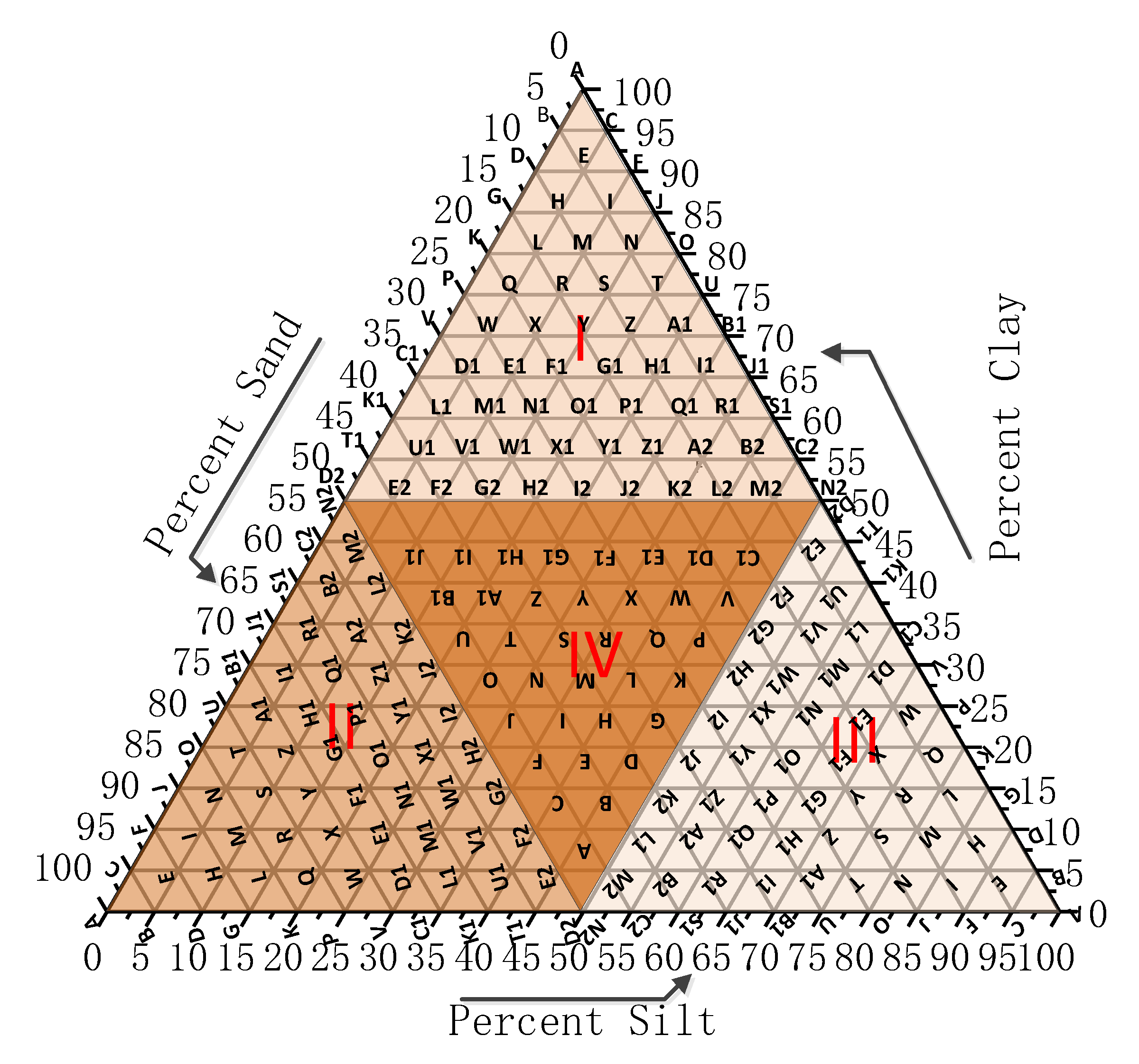
Figure 2.
Maximum bound water fraction (MBWF) versus clay percentage. Legend notes: eq (5) and eq (7) indicate that the MBWF is computed by Equation (5) or Equation (7), respectively, and: 1, a sand fraction of 0; 2, a sand fraction of 30%; and 3, a sand fraction of 60%.
Figure 2.
Maximum bound water fraction (MBWF) versus clay percentage. Legend notes: eq (5) and eq (7) indicate that the MBWF is computed by Equation (5) or Equation (7), respectively, and: 1, a sand fraction of 0; 2, a sand fraction of 30%; and 3, a sand fraction of 60%.

Figure 3.
Simulated real parts of typical soil samples for different models. A solid line is used for soil texture cases in Section I or II; and a dashed line is used for soil texture cases in Section III or IV. “II-I-L” stands for I sample from Section II at the L-band.
Figure 3.
Simulated real parts of typical soil samples for different models. A solid line is used for soil texture cases in Section I or II; and a dashed line is used for soil texture cases in Section III or IV. “II-I-L” stands for I sample from Section II at the L-band.

Figure 4.
Simulated imaginary parts of typical soil samples for different models. A solid line is used for soil texture cases in Section I or II; and a dashed line is used for soil texture cases in Section III or IV Section. “III-H-L” stands for H sample from Section III at the L-band.
Figure 4.
Simulated imaginary parts of typical soil samples for different models. A solid line is used for soil texture cases in Section I or II; and a dashed line is used for soil texture cases in Section III or IV Section. “III-H-L” stands for H sample from Section III at the L-band.
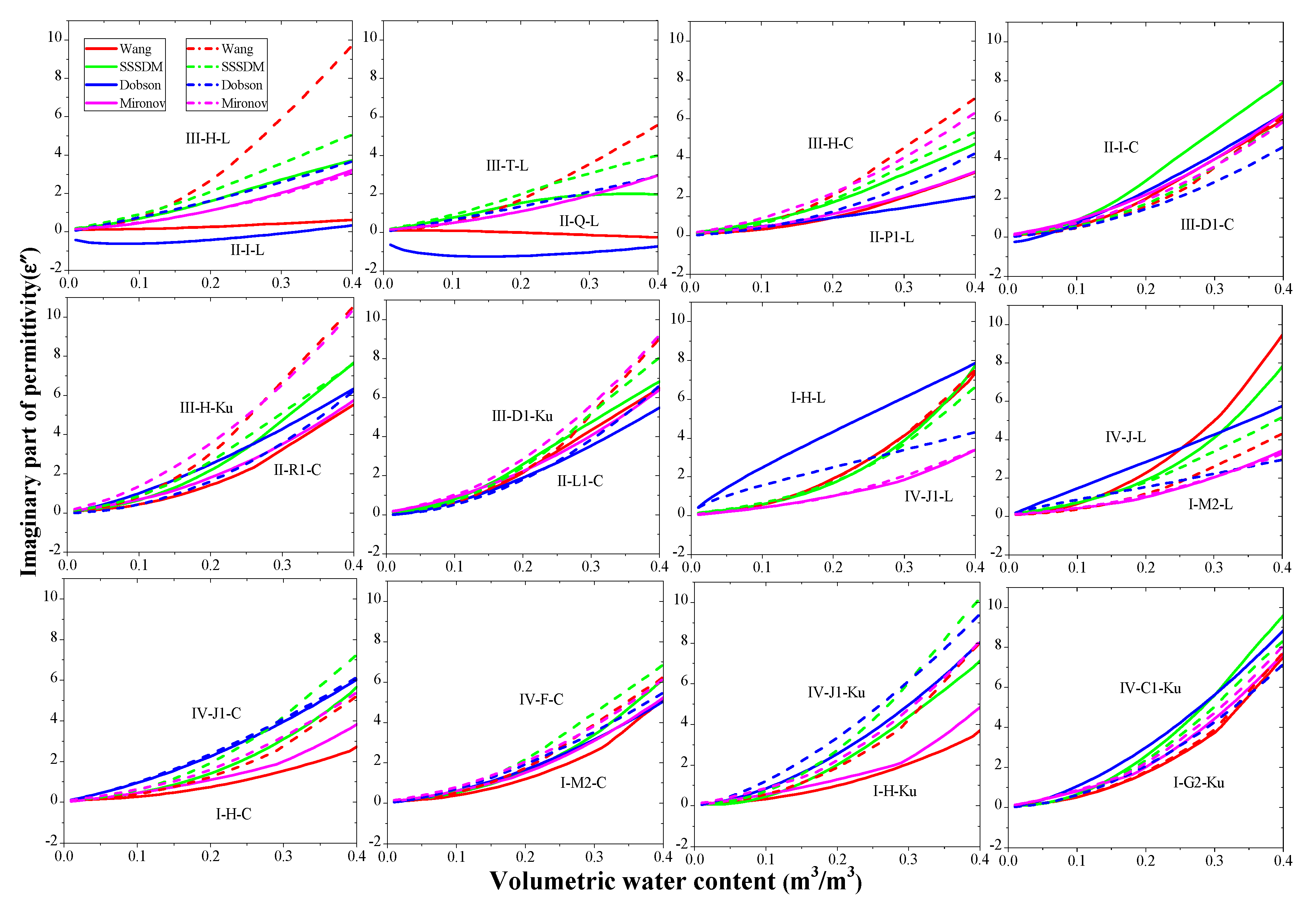
Figure 5.
The simulations of the real parts for different soil texture types under the same model. Top panels—sand content constant; middle panels—clay content constant; bottom panels—silt content constant. ‘H(I)’ is the ‘H’ sample from I soils. A solid line is used for the L-band and a dashed line is used for the Ku-band.
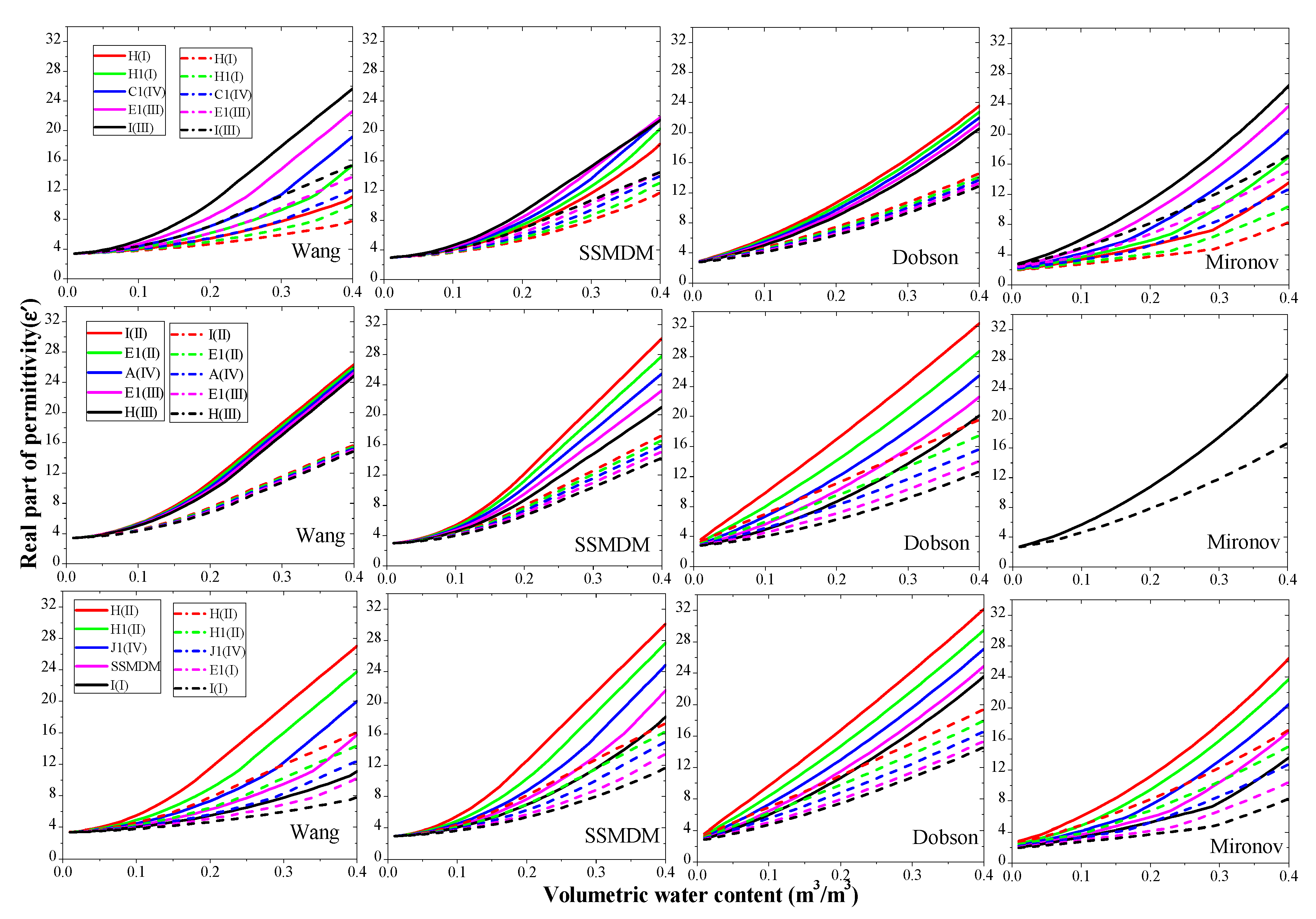
Figure 6.
Deviations in the soil moisture estimates by different models for typical soil samples. The numbers (from ‘1′ to ‘6′) were explained earlier in Section 2. The black straight line represents the soil moisture estimate accuracy requirement of 0.04 m3/m3.
Figure 6.
Deviations in the soil moisture estimates by different models for typical soil samples. The numbers (from ‘1′ to ‘6′) were explained earlier in Section 2. The black straight line represents the soil moisture estimate accuracy requirement of 0.04 m3/m3.

Figure 7.
Deviations in the soil moisture retrievals by soil texture. Top panels—sand content constant; middle panels—clay content constant; bottom panels—silt content constant. ‘H(I)→H1(I)’ is the ‘H’ sample from Section I, which is used as the input soil texture for the soil dielectric model to construct the lookup table (LUT). The ‘H1′ sample from Section I is the input soil texture for the same soil dielectric model to retrieve the soil moisture.
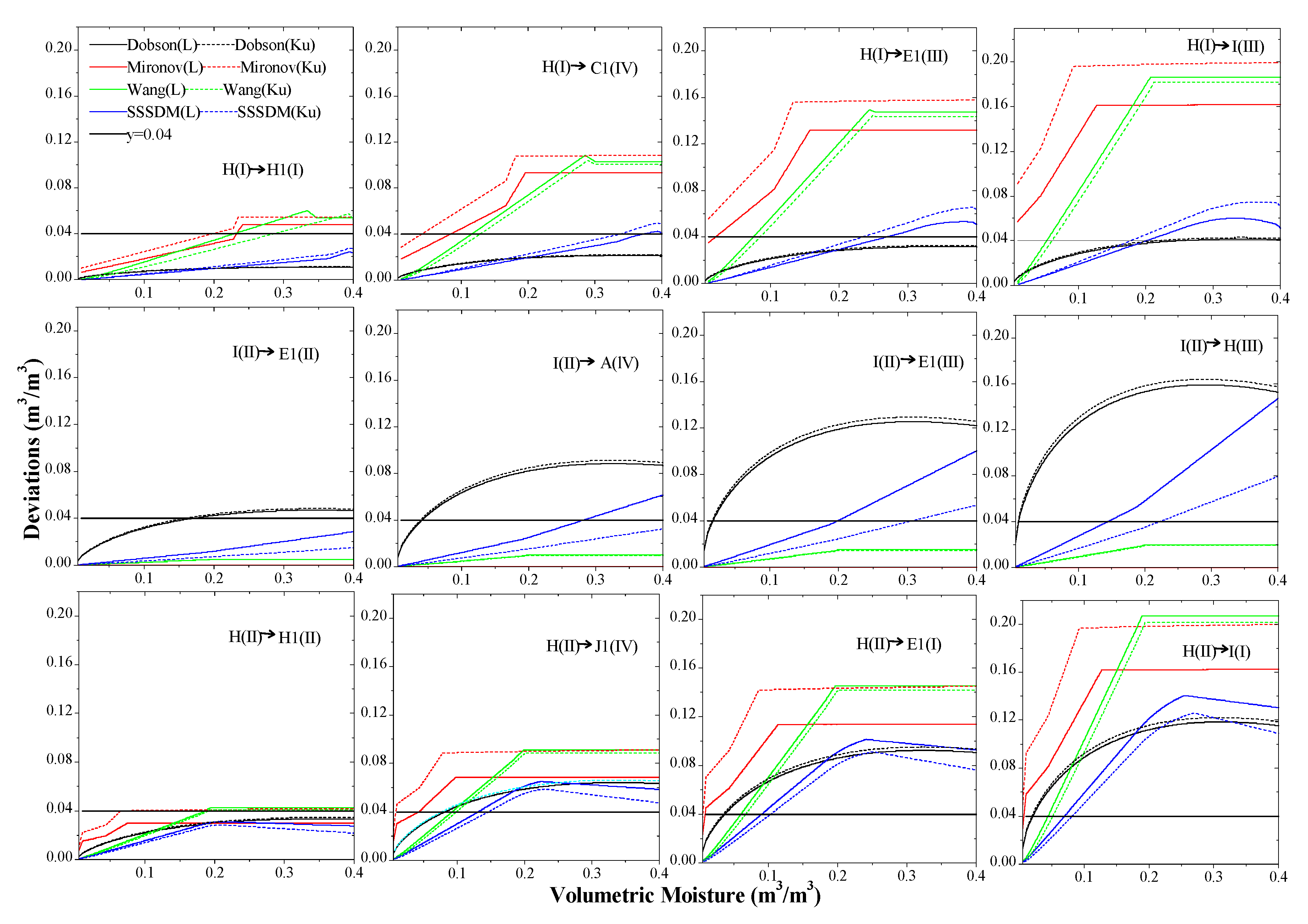
Table 1.
Soil texture cases of the existing validations.
| Sources of Measurements | Sand (%) | Silt (%) | Clay (%) | Sources of Measurements | Sand (%) | Silt (%) | Clay (%) | ||
|---|---|---|---|---|---|---|---|---|---|
| From ref [25] | Forest soil | 57.4 | 32.1 | 10.5 | From ref [27] | Silt loam | 8 | 71 | 21 |
| Natural soil | 72.2 | 24.3 | 3.5 | From ref [26] | Sandy loam | 62 | 24 | 14 | |
| Sand soil | 92.7 | 6.7 | 0.6 | From ref [23] | silty clay loam | 11 | 62 | 27 | |
| From ref [12] | Harlingen clay | 2.0 | 37.0 | 61.0 | From ref [7] | Sample 1 | 51.51 | 35.06 | 13.43 |
| F2 | 56.0 | 26.7 | 17.3 | Sample 2 | 41.96 | 49.51 | 8.53 | ||
| H7 | 19.3 | 46.0 | 34.7 | Sample 3 | 30.63 | 55.89 | 13.48 | ||
| Yuma sand | 100 | 0 | 0 | Sample 4 | 17.16 | 63.84 | 19.00 | ||
| Vernon clay loam | 16.0 | 56.0 | 28.0 | Sample 5 | 5.02 | 47.60 | 47.38 | ||
| Miller clay | 3.0 | 35.0 | 62.0 | From ref [10] | Silty sand (D) | 77 | 9 | 14 |
© 2020 by the authors. Licensee MDPI, Basel, Switzerland. This article is an open access article distributed under the terms and conditions of the Creative Commons Attribution (CC BY) license (http://creativecommons.org/licenses/by/4.0/).
Share and Cite
MDPI and ACS Style
Liu, J.; Liu, Q. Soil Moisture Estimate Uncertainties from the Effect of Soil Texture on Dielectric Semiempirical Models. Remote Sens. 2020, 12, 2343. https://doi.org/10.3390/rs12142343
AMA Style
Liu J, Liu Q. Soil Moisture Estimate Uncertainties from the Effect of Soil Texture on Dielectric Semiempirical Models. Remote Sensing. 2020; 12(14):2343. https://doi.org/10.3390/rs12142343
Chicago/Turabian StyleLiu, Jing, and Qinhuo Liu. 2020. "Soil Moisture Estimate Uncertainties from the Effect of Soil Texture on Dielectric Semiempirical Models" Remote Sensing 12, no. 14: 2343. https://doi.org/10.3390/rs12142343
Note that from the first issue of 2016, this journal uses article numbers instead of page numbers. See further details here.