Ka-Band Doppler Scatterometry over a Loop Current Eddy
by
 , , , , ,
Ernesto Rodríguez
1,* ,
,
Alexander Wineteer
1,
Dragana Perkovic-Martin
1,
Tamás Gál
1,2,
Steven Anderson
3,
Seth Zuckerman
3,
James Stear
4 and
Xiufeng Yang
4 1
Jet Propulsion Laboratory, California Institute of Technology, Pasadena, CA 91109, USA
2
Gata Computing LLC, Los Angeles, CA 91101, USA
3
Areté, Northridge, CA 91324, USA
4
Chevron Energy Technology Company, Houston, TX 77002, USA
*
Author to whom correspondence should be addressed.
Remote Sens. 2020, 12(15), 2388; https://doi.org/10.3390/rs12152388
Submission received: 17 June 2020
/
Revised: 17 July 2020
/
Accepted: 22 July 2020
/
Published: 24 July 2020
(This article belongs to the Section Ocean Remote Sensing)
Abstract
:Doppler scatterometry is a promising new technique for the simultaneous measurement of ocean surface currents and winds. These measurements have been recommended by the recent US NRC Decadal Review for NASA as being priority variables for the coming decade of Earth observations. In addition, currents and winds are useful for many applications, including assessing the operating conditions for oil platforms or tracking the dispersal of plastic or oil by surface currents and winds. While promising, Doppler scatterometry is relatively new and understanding the measurement characteristics is an important area of research. To this end, Chevron sponsored the deployment of DopplerScatt, a NASA/JPL Ka-band Doppler scatterometer, over instrumented sites located at the edge of a Gulf of Mexico Loop Current Eddy (LCE). In addition to in situ measurements, coincident synoptic maps of surface currents were collected by the Areté ROCIS instrument, an optical current measurement system. Here we report on the results of this experiment for both surface currents and winds. Surface current comparisons show that the Ka-band Current Geophysical Model Function (CGMF) needs to include wind drift currents, which could not be estimated with prior data sets. Once the CGMF is updated, ROCIS and DopplerScatt show good agreement for surface current speeds, but, at times, direction differences on the order of 10° can occur. Remote sensing optical and radar data agree better among themselves than with ADCP currents measured at 5 m depth, showing that remote sensing is sensitive to the the currents in top 1 m of the ocean. The LCE data provided a unique opportunity to study the effects of surface currents and stability conditions on scatterometer winds. We show that, like Ku-band, Ka-band estimates of winds are related to neutral winds (and wind stress) and are referenced relative to the moving frame provided by the current. This is useful for the study of air-sea interactions, but must be accounted for when using scatterometer winds for weather prediction.
1. Introduction
Ocean surface currents and winds are essential climate variables that govern the flux of heat and gases between the ocean and the atmosphere. The importance of these variables has been highlighted by the latest US National Academy of Sciences Decadal Survey report for NASA [1], which identifies these variables as a suitable target for an Earth Explorer mission in the next decade. Pencil-beam Doppler scatterometry has been proposed as a method for making these measurements from space in the Winds and Currents Mission (WaCM) concept [2] and the ESA SKIM [3] mission. As a precursor to these spaceborne instruments, the NASA Jet Propulsion Laboratory (JPL) has developed and flown the Ka-band DopplerScatt instrument [4] under NASA’s Instrument Incubator Program (IIP-13) and Airborne Instrument Technology Transition (AITT-16).
In addition to global applications, which require satellite measurements, regional high-resolution measurements of ocean vector winds and currents are important for both science and applications. The ocean sub-mesoscale, whose feature wavelength range spans from hundreds of meters to tens of kilometers, is the scale at which much of the vertical ocean circulation occurs [5], much of it driven by local winds. The Sub-Mesoscale Ocean Dynamics Experiment (S-MODE), selected in 2018 as a NASA Earth Ventures Suborbital (EVS) Mission, will use the DopplerScatt instrument, along with other airborne and in situ sensors, to improve our understanding of the ocean sub-mesoscales.
Aside from purely scientific applications, ocean surface currents and winds have important commercial and social applications. The dispersal of ocean surfactants and debris is governed by both winds and currents. For instance, for the propagation of the oil plume resulting from the Deep Water Horizon oil spill in the Gulf of Mexico (GoM), it was shown that the “prevailing winds, through the drift they induced at the ocean surface, played a major role in pushing the oil toward the coasts along the northern Gulf, and, in synergy with the Loop Current evolution, prevented the oil from reaching the Florida Straits.” [6]. Oil platform operations in the GoM are also affected by strong currents, especially during installations, which are vulnerable in part because they require Remotely Operated Vehicles (ROVs) that typically have an operating limit of about 0.75 m/s currents [7].
Doppler scatterometry offers an promising technique for measuring surface currents and winds simultaneously and the work presented in [4] showed promising comparisons between DopplerScatt observations and models (the Navy’s NCOM model for surface currents and a high-resolution RSMAS atmospheric model). However, several questions remained after this initial work: How well did wind and current measurements compare against in situ observations of winds and currents? How significant was the wind drift contribution to the relationship between radar Doppler and surface currents (the method used in [4] could not estimate this contribution due to lack of in situ data)? Ku-band data has been shown to be related to wind stress (or, equivalently, neutral winds); does this relationship also apply at Ka-band (i.e., does surface stability affect the relationship between buoy winds and scatterometer wind)? Addressing these questions successfully is required for scaling up the DopplerScatt airborne measurements into a global wind and current mission, as called for by the NASA decadal survey.
In this paper, we present the first steps towards answering these questions using a validation experiment for the DopplerScatt instrument undertaken in partnership between JPL, Chevron, and Areté over a Loop Current eddy, named “Quantum Eddy”, conducted in March, 2018. The Gulf of Mexico (GoM) was selected since the strong Loop Current eddies provided a clear signal of a frontal system with significant current and sea surface temperature discontinuities typical of strong mesoscale eddies, and the results also had applications to oil platform operations in the GoM. The strong current fronts associated with Loop Current eddies provided an environment suitable for assessing the DopplerScatt surface current estimates in the presence of strong and weak currents, and in the presence of significant horizontal current shear, as well as different current measurement depth. As an independent measurement of the DopplerScatt surfaces currents, we used surface currents measured by the mature Remote Ocean Current Imaging System (ROCIS) [8], as well as near-surface ADCP measurements from a stationary buoy. The presence of independent ROCIS information also allowed for the validation of the corrections that must be applied to the DopplerScatt currents to remove gravity wave modulation effects.
While a comparison of DopplerScatt winds with buoy measurements were presented in [4], an open question is whether the Ka-band measurements reflect surface wind stress (or, equivalently, neutral winds), as has been observed at Ku-band [9]. It is already known that Ka-band returns show a temperature dependence at low temperatures [10]. Warm surface temperatures drive unstable atmospheric boundary conditions, which in turn lead to reduced winds at 10 m relative to neutral conditions. In addition, the surface currents will modify the stress, since it is measured relative to the moving surface, but not the buoy winds [9,11]. The data collected in this experiment can thus serve to understand the relationship between Ka-band neutral winds and the true 10 m winds measured by buoys and assess the relative contributions of surface currents and atmospheric stability.
In Section 2, we review the measurement principles of the DopplerScatt and ROCIS instruments, and describe the in situ instrumentation and environmental conditions encountered during the experiment. The experimental results for both winds and current comparisons between DopplerScatt, ROCIS, and in situ data is presented in Section 3. The implications of these results on Doppler scatterometry are then discussed in Section 4.
2. Experiment Description
2.1. The DopplerScatt Instrument
The DopplerScatt instrument [4] (see Figure 1), developed under NASA’s Instrument Incubator Program (IIP), is a Ka-band pencil-beam Doppler scatterometer that measures ocean surface currents and winds simultaneously. The instrument, hosted on the NASA Armstrong Flight Research Center’s (AFRC) King Air B200 platform, uses a spinning antenna with a 56° nominal elevation angle to illuminate a 600 m footprint on the ground when flying at 28,000 ft. As the antenna rotates and the airplane moves, the scan will illuminate a 25 km swath and revisit any point on the ground from multiple azimuth look directions. At a nominal air speed of 250 knots, an altitude of 28,000 feet, and data collection time of more than 4 h, the system can collect data over an area 45,000 km in one data collection sortie. Since Ka-band will propagate through clouds (but not rain), the system is not constrained by clear weather requirements typical of optical sensors. Due to the pencil-beam geometry and narrow beam, DopplerScatt does not suffer from the swath-width limitations of typical side-looking Synthetic Aperture Radar (SAR) systems. Below, we provide a high-level summary of the the measurement principles for DopplerScatt, and refer the reader to Rodríguez et al. [4] for details of the measurement physics and data processing.
DopplerScatt uses pulse-pair phase differences to estimate the relative velocity along the look direction(usually called the radial velocity) between the airplane and theBragg resonant surface capillary waves (0.5 cm wavelength) that dominate the backscattering of the radar signal [12]. Using a high-precision Inertial Motion Unit (IMU) and antenna pointing information, the airplane contribution to the radial velocity is removed, and the resulting residual radial velocity vector is projected to the ground to obtain the ocean surface radial velocity. DopplerScatt is very sensitive to pointing errors between the aircraft velocity vector and the antenna boresight. This pointing offset has been calibrated using repeat passes in opposite directions. as described by Rodríguez et al. [4]. An additional source of error is in the determination of the platform heading in geographic coordinates. The specification of the heading error after blending IMU and GPS data is less than one-hundredth of a degree, which leads to insignificant errors. Finally, as described in Rodríguez et al. [4], the measurement is very insensitive to platform elevation errors.
The phase velocity of capillary waves is the source of the residual Doppler signal. Neglecting larger gravity waves for the moment, this phase velocity is the vector sum of the surface current, averaged over a fraction of a centimeter, and the capillary wave velocity. For free capillary waves, this velocity has a peak along the wind direction and the waves travel at a phase speed of ∼31 cm/s, as determined by the capillary wave dispersion relation. When longer surface gravity waves are present, the total radial velocity vector will include the contribution from the gravity wave radial velocity. If the capillary contribution was uniform over the gravity waves, the effect of surface waves would average out when the radar footprint contains many wave periods, as it does for DopplerScatt data, which is processed at spatial resolutions from 200 m to 400 m. However, due to hydrodynamic modulation by the gravity waves, as well as wind roughening downwind of the wave peaks, the amplitude of the capillary waves will increase towards the wave crests and decrease towards the troughs. Since the measured residual radial velocity is weighted by the scattered power, and the backscatter cross section is proportional to the amplitude of the Bragg resonant capillary waves, the net effect will be to have a residual velocity contamination in the direction of the gravity wave propagation [4]. This residual effect, which depends on the wind speed, must be removed along with the capillary wave propagation velocity in order to recover the surface currents. To date, the correction, which we call the Current Geophysical Model Function (CGMF), has been determined on a limited number of flights without extended ground truth collected prior to the March 2018 deployment [4]. The availability of ROCIS data presents an excellent opportunity for improving the DopplerScatt CGMF, as we will discuss in Section 3.2.
In addition to surface current estimates, the measured normalized backscatter cross sections, , can be used to estimate surface neutral stability 10 m winds. The measurement principle is summarized in [4,13]. Previous deployments have demonstrated good wind retrieval skill, and the results from the instrument are used as an input to the CGMF correction, so that no independent source of wind measurements is required for estimation of the surface currents.
Prior to the March 2018 deployments, DopplerScatt had used a lower resolution mode (5 MHz) for data collection. For March 2018 deployment, we introduced a higher resolution mode (10 MHz) that was expected to improve measurement performance and the capability of inferring surface gravity wave spectra. The new mode was flown on 24, 26, and 27 March, while the old mode was flown on March 25. Both modes were calibrated using repeat tracks, following the methodology described by [4]. The performance results presented in Section 3.2 show that the higher resolution mode did indeed improve performance significantly.
2.2. The ROCIS Instrument
ROCIS is an airborne optical system that measures surface currents by utilizing time-series imagery to observe the Doppler shift of surface gravity waves. (See Figure 1 for measurement geometry and concept illustration.) Two cameras, one fore and one aft, look at a grazing angle of 38°, and collect panchromatic wave imagery at a rate of 2 Hz. The images are each georectified to the water surface with a ground sample resolution of 1 m and individual datacubes are built up at specified retrieval locations. Each datacube is 256 m × 256 m and contains between 60 s and 120 s of dwell, depending on aircraftaltitude and flight speed. Retrieval locations can either be in abread crumb trail along the flight path, providing a real-time quicklook product, or the imagery can be post-processed using a grid of locations to produce acontiguous field of current measurements across the entire imaging swath of the system. In deep water, ocean waves are governed by the linear dispersion relation:
where k is wavenumber, g is acceleration due to gravity, is frequency, and is current vector. For each datacube, a three dimensional Fourier transform is computed yielding a power spectral density (PSD). ROCIS computes the surface current by fitting the Doppler shift of the observed wave energy in the spectrum to the dispersion relation given by Equation (1). For this analysis, ROCIS data was post-processed to yield independent current estimations on a 256 m square grid of non-overlapping tiles.
This technique is subject to two systematic sources of velocity error occur due to misalignment between the camera and the Inertial Navigation System (INS) boresight. Heading boresight errors lead to errors in the across-track component of the current. Mapping platform height uncertainty leads to a bias in the along-track component of the surface currents. These systematic errors are in aircraft coordinates and are independent from the true surface current (or wind direction). Thus, the errors become very apparent in the data from reciprocal flight lines or simply when the heading turns quickly. The ROCIS lines collected for this program are back and forth, but not directly overlapping, so no direct reciprocal is available. Due to the small aircraft and lower aircraft speed and flight altitude, ROCIS is more sensitive to these errors than DopplerScatt. These unquantified potential sources of error should be kept in mind when discussing the results below.
In the presence of upper-level shear, is a weighted average [14,15] over the top few meters of the Eulerian surface current. The effective velocity is given by
where is the true current current at a function of depth. Note that classical Stewart and Lovejoy [14] result in this equation will not apply in the presence of wave breaking. ROCIS uses multiple surface wave wavelengths to form an average current estimate [8], and the effective depth of the estimated current is representative of the average current over the top few meters. Due to averaging over the collected data, one independent surface current measurement is obtained every 675 m [8].
2.3. Experiment Site and Environmental Conditions
The Loop Current (LC), the major circulation feature in the Gulf of Mexico (GoM), periodically sheds long-lived warm anti-cyclonic eddies, called Loop Current Eddies [16] (LCE’s). LCE’s are large persistent high velocity features (2–4 knots, 1–2 m/s) whose evolution is difficult to model [17]. They play significant roles in the transport of fish larvae and hurricane intensification. They are of special interest to the GoM oil industry as high currents can stress, or even shut down, oil platforms and can also play a significant role in the dispersal of oil spills [6,17]. Currents derived from the satellite altimeter constellation can provide low-resolution monitoring of these features [18], but additional spatial resolution is important for planning and forecasting. Although there has been a lot of effort in forecasting LCEs, current models still suffer from limitations in forecasting skill [17].
The ability to image through clouds and fog at any time of day or night, together with the high-resolution, wide mapping capability provided by the DopplerScatt system has the potential to bring significant benefits to the real-timemonitoring of LCEs. To assess DopplerScatt’s capabilities, Chevron funded a field experiment over one such LCE, named “Eddy Quantum”. Eddy Quantum separated from the LC on early November 2017, and split in two in late November. The northern eddy, Quantum I, reattached to the Loop Current several times following its initial detachment, with its latest separation in May 2018. The DopplerScatt field deployment consisted of four sorties, collected from 24 March to 27 March 2018, when the eddy was located as shown in Figure 2. ROCIS coincident data were collected on 25 and 26 March.
The experiment site was located to overlap data collected by a Fugro SEAWATCH METIS buoy located at latitude 26.9°, longitude −90.5°. The buoy provided data every 30 min for wind speed and direction, significant wave height and wave propagation direction (see Figure 3), and ADCP current data at various depths near the surface (see Figure 4). There are challenges due to aliasing of surface wave motion in measuring current shears very near the surface, and these should be borne in mind when examining the detail surface current shear measured by the ADCP. Wave conditions for both days had significant wave height of ∼1 m. The wave direction, which was along the wind direction for 2018-03-25, (see Figure 5), steered by only ∼10° on the 26th, while the winds direction changed to about 45° west of north, leading to wind and wave directions having significant differences on 2018-03-26.
In addition to the METIS buoy, the BW Pioneer buoy (NDBC Station 42360), located at latitude 26.672°, longitude −90.471°, lay in the middle of the southern DopplerScatt swath and provided standard meteorological wind and wave information. The upper panel of Figure 3 shows good wave height agreement between the two buoys. The NDBC buoy did not provide wave direction (provided by the METIS buoy), but did provide dominant wave period, shown in the lower panel of Figure 3. The dominant wave periods during the DopplerScatt observations were typical of wind-driven waves. This was corroborated by wave information from the METIS buoy that estimated that swell only contributed a few centimeters to significant wave height.
A comparison of DopplerScatt’s surface currents at the same location, and at roughly the same time (time differences on the order of one hour), was provided by ROCIS surface current measurements. Due to the long cruise distance to reach the Quantum eddy, ROCIS collected a swath of approximately 5 km by 100 km using seven passes on 25 and 26 March. The data were first processed in quick look mode and reprocessed at denser spatial sampling by Areté Associates and provided to JPL for comparison with DopplerScatt velocity data.
On the first of joint data collection days (2018-03-25), DopplerScatt separated its swaths so that there was very little overlap. The result was that no swath fully covered the ROCIS swath. As shown in Figure 5, the winds were blowing in a northerly direction, so that measurements were close to either upwind (against the wave direction), or downwind (along the wave direction). Since the data were in the outer part of the swath, the azimuth diversity required to estimate vector velocities was small, and the errors in the estimated velocity were expected to be at a maximum. The data collected during this day also used a low-resolution mode that had been used in prior data collections.
In addition to the in situ measurements described above, glider and FAST (Fast Autonomous Survey Technology) Eddy System measurements of currents at depth were also collected, but not used for this study, which concentrates on surface currents.
3. Results
3.1. Wind Estimation Results
3.1.1. Wind Processing
The wind processing for DopplerScatt largely follows [4], but has been improved to use the expected errors to guide retrievals, especially in the regions near the nadir track. The wind inversion process minimizes the differences between observed values of and those predicted by an empirical wind GMF, which depends on wind speed and observation direction. Initial processing with the GMF given in [4] showed that, at high wind speeds, DopplerScatt overestimated the buoy wind speed by about 10%. This difference has been accounted for by an improvement in the antenna calibration and refined estimates of the system noise floor, combined with better knowledge of high wind speed GMF uncertainties due to limited data prior to 2018. This calibration update can be incorporated into the GMF results of [4] by introducing an effective linear correction (in dB) to the measured . This correction was designed to create no change at low wind speeds and a 1 dB change (relative to the previous GMF) at 10 m/s wind speeds. The DopplerScatt GMF is currently being tuned with improved calibration and data collected after this experiment, and the results will be reported elsewhere. The conclusions in this paper are not altered significantly when using this improved GMF over the linear correction, which we provide here for continuity with the GMF in [4].
3.1.2. Wind Data Overview
DopplerScatt collected data in two wind regimes during this deployment. On 24th March, we measured moderate winds speeds averaging approximately 10 m/s. The 25th brought lower wind speeds of approximately 5 m/s on average. Winds picked back up on the 26th and 27th, with speeds of about 9 and 11 m/s. A histogram of wind speeds as retrieved by DopplerScatt for each flight is shown in Figure 6, along with the corresponding NOAA Blended SeaWinds estimated wind speeds [19,20]. NOAA SeaWinds is a 0.25° degree, global blended model-observation product based on GFS model data and all available wind observations. At this resolution (∼25 km), we can expect a much smoother wind field compared to the 400 m posting estimates produced by DopplerScatt.
Figure 7 plots NOAA OSPO processed sea surface skin temperature (SST), as estimated from NOAA’s Visible Infrared Imaging Spectrometer (VIIRS) on the Suomi NPP spacecraft and interpolated to 1 km resolution. The Figure represents a four-day average, required to obtain coincident, near cloud-free coverage. Despite the time averaging, the resulting SST field shows structure within the eddy at mesoscales that lends hope to investigating the interactions between SST and the wind. Flight areas where DopplerScatt winds were measured are overlaid (rectangles labeled “a” and “b”). Two buoys with comparison wind measurements in the flight region are labeled “c” and “d”. The buoy labeled “c” is a Fugro buoy operated by The Chevron Corporation, which provided data for this study. The buoy labeled “d” is listed on the National Data Buoy Center as buoy #42360.
We focus on the two flight dates with coincident ROCIS data: one for low winds, on the 25th, and one for moderate winds, on the 26th. Figure 8 shows the spatially gridded averaged wind field for all flight lines for the 25th, on the left, and for the 26th, on the right. On the 25th, DopplerScatt measured low average wind speeds and directions towards the North. The most notable feature in the winds from the 25th is the distinct jump in wind speeds near −90.5° longitude (bottom left) of the measurement area, coincident with the edge of Quantum Eddy (see current discussion below). Surface currents at longitudes greater than −90.5° in the image are strong due to the eddy, and are aligned with the wind. The currents create a moving reference frame for the wind-driven capillary waves measured by the scatterometer, lowering surface stress, as we discuss in greater detail below. A similar feature occurs in the North-South oriented flight line on the 25th, where equivalent neutral wind speeds suddenly decrease at the eddy front, near 28.5° North latitude. In this case, the currents are nearly perpendicular to the wind direction, so we would not expect the reference frame effect that we saw in the East-West flight lines. Instead, strong negative downwind SST anomalies (negative downwind SST gradients) have been shown to correlate with wind convergence, likely due to a tilting of the planetary boundary layer [21]. Comparing Figure 7 to Figure 8 qualitatively supports a correlation between SST and wind at SST fronts.
Figure 9, top zooms on the wind field as estimated by DopplerScatt on the 25th for the East-West flight lines. The two flight lines that were pieced together to form this mosaic were taken about 45 min apart, leading to the discontinuity in wind speeds along the center of the image. The strong jump in wind speed associated with the edge of the warm-core eddy is now revealed in detail. The wind direction, however, remains consistently northward across the flight area across the front. This is because the wind direction and surface currents were aligned, leaving the resulting wind stress direction unchanged. As is typical to pencil beam scatterometers, errors are highest near the center of the swath due to poor measurement geometry.
Figure 9, bottom zooms into the wind field from two flight lines for the 26th, showing winds of about 10 m/s towards the North-West. Due to strong tail and head-winds, sampling along the center line was sparse, leading to gaps and greater noise, so this area is masked out. Interestingly, the wind patterns observed on the 26th are completely different from those observed on the 25th, despite mapping nearly identical regions. The sharp eddy boundary is no longer apparent in the wind speed, although a gradient does appear along the Eastern side of the figure. If we look at the surface currents measured by DopplerScatt for these two dates, as seen in Section 3.2, we see a similar change in the eddy boundary: the currents on the 25th have a much sharper edge than on the 26th. We investigate this feature more closely in the following section.
3.1.3. Buoy Wind Comparisons
Two buoys were found in our flight region, one with data provided by the Chevron corporation (marker “c” in Figure 7) and another from the National Data Buoy Center (marker “d” in Figure 7). We aligned the measurements made by the buoys and DopplerScatt in time and averaged DopplerScatt data in a region consistent with the time-averaging of buoy measurements. With buoy measurements every ten minutes, that corresponds to an area averaging of about 6 square kilometers in DopplerScatt data, assuming 10 m/s wind speeds. Each flight pass over the buoy was used as an independent data point, and with about six lines each day and four days of data, we find a total of around 24 data points for each buoy. The North-South lines were omitted but all East-West lines were used. The Southern-most East-West lines were not directly over the Chevron buoy and the nearest point was used (typically within 10 km), leading to some colocation error.
There is evidence that scatterometers are sensitive to the relative velocity between surface winds and surface currents, and is referred to as the “relative wind” [22]. Furthermore, scatterometer wind measurements are tuned to retrieve “equivalent neutral winds”; i.e., neutrally-stable marine-atmospheric boundary layer winds at 10 m above the ocean surface [23]. To a lesser degree, ocean surface temperature causes changes in the viscosity and surface tension of water, leading to changes in the generation of capillary waves that scatterometers are sensitive to, as well as the dielectric constant of water at Ka band [10]. While we will consider the effects of surface currents and atmospheric stability, the effect on capillary wave viscosity, surface tension, and the dielectric constant are only important at low temperatures, and not sampled by this experiment.
Under stable conditions, scatterometer winds are an adequate approximation of the true ten meter wind speed, but cases exist where this approximation breaks down. The first case is when the surface current, , is large, typically in places with strong geostrophic flow like the Western Boundary Currents [9], near river outflows [4], and in areas of strong tides [22]. A second place where this approximation breaks down is when surface boundary layer conditions are not neutral. Since scatterometer winds are measured at a reference height of (typically) 10 m, changes in the vertical density profile lead to changes in 10 m wind speed. Non-neutral conditions are associated with atmospheric density stratification and typically occur when there is a significant positive temperature gradient between the ocean surface and atmospheric temperature.
The atmospheric stability and surface current relative wind effects are separated by referencing the wind velocity vector at height z above the displacement height, , relative to the moving frame provided by the current velocity, . In this moving frame, the height dependence of the wind speed depends solely on the atmospheric stability conditions. Assuming the well-known logarithmic wind profile [24,25]
where is the friction velocity, is the von Karman constant, is the roughness length, and L is the Monin-Obukhov scale length [26]. is an atmospheric stability term for momentum that disappears under neutral wind conditions. Considering these terms, it is clear that (1) we can expect a one-to-one modulation of winds due to underlying surface currents under neutral, typical conditions (currents << winds); (2) winds vary logarithmically with reference height, and (3) winds will vary depending on atmospheric stratification. Since buoy measurements are typically taken in non-neutral conditions, at a measurement height other than 10 m, and are not relative to surface currents, all of these effects will need to be corrected for when making comparisons to scatterometer winds. One important note to emphasize here is that both the winds and currents in Equation (3) are vector quantities. The one-to-one relationship we discuss assumes winds and currents are aligned (moving in the same direction). If this is not the case, the vector addition of the two complicates the one-to-one relationship.
These corrections are especially important in this work, due to the large currents and SST anomaly from Quantum Eddy (Figure 7). Since the eddy current was generally aligned with the wind in our flight area, we can hypothesize that current effect will be to bias the estimated winds low. On the other hand, the warm water underlying cooler air will induce surface layer instability that will cause scatterometer winds to be higher than buoy measured winds. Since the currents in the eddy were quite strong (>1 m/s), and typical surface stability corrections are <0.5 m/s, we might expect a net decrease in DopplerScatt-measured wind speeds over the eddy when compared to buoy winds.
The contribution of currents to DopplerScatt winds can be estimated directly using the DopplerScatt estimated surface currents. We add measured vector currents back into the vector wind measurement when the correction is desired. To correct for atmospheric stability, we used the Liu-Katsaros-Businger (LKB) algorithm [23], VIIRS SST, and buoy atmospheric temperatures. We assumed a relative humidity of 80%, since measurements were unavailable. While VIIRS SST provides high-resolution, synoptic coverage over our flight area, atmospheric temperatures were assumed constant over the flight region and taken from buoy point measurements. Figure 10 shows the progression of the stress equivalent neutral wind (SENW) field from the 25th (top) to neutral wind (ENW) (middle) to 10-m wind speed (bottom). Since DopplerScatt surface currents have large errors near the center of the swath, these areas are masked in the two bottom panels (b, c) in Figure 10.
Using the two corrections shown in Figure 10, we compared DopplerScatt true 10 m winds to buoy measured true 10 m winds for the four flight dates. The upper panel of Figure 11 shows this comparison for wind speed, while the lower panel compares wind direction. The time correlation between DopplerScatt and the buoys is quite good, with changes in wind speed/direction being tracked by both the buoy and DopplerScatt. We have also collocated radiometer wind speed measurements from the SSMI F16, F17, F18, GMI, and AMSR-2 radiometers. These measurements are satellite estimates of wind speed at a much coarser resolution than DopplerScatt and are plotted in green triangles when available. Since they are also sensitive to stress, rather than the actual winds, the radiometer estimated wind speed is uniformly lower than the buoy estimates. Additional scatter is probably due to coarse radiometer resolution over a frontal region.
Another way of looking at the same comparison is shown in Figure 12, where the time dependence has been removed and only speeds and directions are compared. These comparisons reveal an excellent agreement between DopplerScatt and buoy measurements with RMS differences of 0.82 m/s in speed (Figure 12, left) and 6.8 degrees in direction (Figure 12, right). The slopes of both the speed and direction comparison in Figure 12 are nearly unity and both have high correlation coefficients.
3.1.4. Scatterometer Wind Dependence on Surface Currents
We follow Plagge et al. [22], to quantify the effects of surface currents and stability on Ka-band scatterometer winds. Taking the magnitude of Equation (3) and expanding in powers of , the residual between the scatterometer winds (10 m neutral winds relative to the moving surface) and buoy winds
(where and are the wind and surface current directions, respectively) is the component of the surface current along the wind direction. In deriving this equation, we have neglected terms of order and higher. If stability conditions are neglected, the difference between DopplerScatt and buoy winds will have a slope of when plotted against . Departures from this relationship will be due to contributions from an unstable boundary layer (and, of course, measurement noise for both winds and currents).
Despite the wealth of scatterometer data and a number of studies, this relationship is not particularly well observed due to a lack of colocated surface currents, wind, and temperature measurements. Using Ku-band QuikSCAT winds and NDBC buoy winds and currents, Plagge et al. [22] found the expected slope of about negative one, but only under neutral boundary layer conditions. When other surface stability regimes were allowed, the slope tended towards zero and correlations reduced significantly.
In the Gulf of Mexico DopplerScatt dataset, we do not have the luxury of removing non-neutral data because all of our data were taken over a strongly unstable ocean eddy boundary layer. Instead, we have used the procedure in [23] and corrected unstable buoy measurements to neutral stability before plotting results in Figure 13. We find that without the LKB stability correction, linear correlation between surface winds and projected surface currents, −0.12, is lower, and the slope, −0.36, is shallower than expected if surface currents are the main source of difference. When the surface stability is accounted for (which would theoretically remove the stability contribution in Equation (4)), the magnitude of the correlation increases to −0.16, and the slope is . The standard error on the slope is about 0.46. These results indicate that the stability term plays comparable role to the surface current under unstable conditions. The significant scatter in the wind speed differences is consistent with the expected measurement errors, so more detailed conclusions cannot be drawn easily.
A similar analysis can be done with wind stress,
where is the wind stress, is the air density, is the drag coefficient, is the true 10 m wind velocity. We used the ECMWF bulk parameterization for [27]. Subtracting buoy-estimated wind stress from DopplerScatt-estimated wind stress gives,
assuming the buoy is not sensitive to surface current velocity and the currents have been projected into the wind direction. We recognize in the term in square brackets in Equation (6) is the stress that would be calculated using the buoy winds, without any surface current contribution. The correction term, in parenthesis, is first order in , with smaller quadratic corrections. This shows that for low wind speeds we can expect smaller difference in wind stress, regardless of projected current speed. For a set wind speed, higher projected currents will result in larger (more negative) differences in stress. Figure 14 shows the results of this analysis using DopplerScatt and buoy wind data, color coded by wind speed. Lines represent Equation (6) for wind speeds of 3, 6, 9, and 12 m/s. There is a qualitative agreement with expectations, but significant data scatter exists and more data is required to go beyond a qualitative assessment.
3.2. Surface Current Estimation Results
Current Geophysical Model Function
The radial velocity measured by DopplerScatt contains a velocity term due to residual surface wave motion which must be removed to recover the surface current velocity [4,28]. Since the amount of contamination is proportional to the Stokes drift current [29], which is largely dependent on the friction velocity measured by scatterometers [30], we parametrize the correction, called the current geophysical model function (CGMF), , as a function of scatterometer neutral wind speed, and , the relative azimuth angle between the radar look direction and the net direction of the surface scatterers. The scatterer net direction, which is mainly along the wind direction, also includes surface current contributions. For DopplerScatt, this direction is equated to the direction determined from the radial velocities, prior to correction with the CGMF. is related to the radar measured radial velocity, , and the surface current, , by
where is a unit vector along the radial direction, and is the neutral 10 m wind. We note that, due to the short capillary wave wavelengths, is the surface current averaged over the top few millimeters. Whereas the ROCIS currents represent the shear-averaged currents over the first few meters, for capillary waves, the lowest order Stewart-Joy phase speed (Equation (2), must be modified to reflect smaller wave contributions [31,32]. Furthermore, recent measurements of the depth dependence of the dispersion relation [33] or the drift speed difference between thin drifters and drifters drogued at about 20 cm [34], show that there can be a substantial difference in current magnitude between the surface current and meter-level currents. Therefore, we expect that to relate surface currents to currents at meter depth, additional corrections must be incorporated into the CGMF.
The availability of coincident ROCIS currents allows us to examine the CGMF. Prior to the deployment described here, no reliable synoptic estimates of the surface current had been available. A first approximation to estimating the CGMF [4] was attempted by binning the radial velocities as a function of wind speed and , and averaging the results over all data collections. Since many different geometries and surface current scenes had been collected, it was expected that the non-wind-driven currents, , would average out; i.e., . However, surface currents whose direction was correlated with the wind direction, such as Eulerian drift currents [15], or Stokes currents that contribute to the wave averaged Doppler velocity [4,28], will not average out, and Equation (7) will become
i.e., the true CGMF is replaced by an Equivalent CGMG (ECGMF), , which includes the contributions of drift currents whose speed, , is a fraction of the wind speed, and whose direction relative to will depend on a boundary and wind speed dependent drift angle, [15]. The wind speed dependence of can be seen in Figure 15, which shows (blue line) the wind speed dependence of the magnitude of the term in the ECGMF, especially marked for lower wind speeds.
Using the ECGMF to compare DopplerScatt currents to ROCIS will not be appropriate since ROCIS will be sensitive to Eulerian wind drift currents at meter scales. To assess the impact of using the legacy ECGMF developed for DopplerScatt, we calculate the ROCIS radial velocity for each DopplerScatt measurement, bin the results as a function of wind speed and to form the quantity
where is the ROCIS measured velocity, and is the CGMF used to correct DopplerScatt measurements to currents’ measurements at the ROCIS depth. will remove surface wave contamination, but retain Eulerian wind-driven currents at meter depth.
To assess the legacy CGMF, we plot in Figure 16 and Figure 17 the empirical estimates for against the legacy CGMF from [4]. Given the limited wind speeds encountered during the GoM deployment, we can only assess the dependence for 1 m/s bins centered at 3 m/s and 4 m/s (2018-03-25, Figure 17) and 6 m/s and 7 m/s (2018-03-25, Figure 16). Referring to the wind speed behavior of the CGMF shown in Figure 15, we see that these wind speed ranges correspond to two different behaviors of the CGMF: for the lower wind speed range, the CGMF depends strongly on wind speed, whereas it stabilizes for the higher wind speeds.
Examining Figure 16, we see that the legacy CGMF fits well in the cross-wind directions, but definitely over-corrects in the up and downwind directions, indicating wind drift currents are included in the ECGMF. For the lower wind speeds in Figure 17 we find that most of the data is well represented by the legacy CGMF, but there is an anomalous cluster of points (highlighted with a colored circle) about of the wind direction that shows significantly higher residual radial velocity than expected. The direction of the shift is consistent with the drift angle of Ekman currents, but its magnitude, as a fraction of wind speed is much larger than previously reported. At this point, we do not know the source of this anomalous behavior, so we do not try to compensate for it. We expected that this will result in excess surface current estimates when the observations are close to the wind direction. This is indeed observed, as will be seen below.
As a first attempt to improve the CGMF, we study the possibility of subtracting a drift current contribution, of the form from the legacy GMF, by estimating using least squares minimization the parameters d and . The results, using all of the data, and only the northern swath (i.e., looking upwind) are given in Table 1. As can be seen from this table, for the moderate wind speed, the magnitude and direction are reasonable, although a bit higher than the ones reported by Ardhuin et al. [15] using HF radars for the estimates. This difference in amplitude might be accounted by the differences in vertical shear experienced by long waves used for HF radar and the short capillary waves used by DopplerScatt. For the lower wind speed, the wind drift percentage is even higher, but the drift angle is nearly at right angle to the wind direction. Since we do not know the source of the anomalous behavior for low wind speeds, we choose to make a simple correction along the wind direction. The coefficients for the one-parameter fit are given in Table 1. As a conservative approach, we assume that the correction is fully implemented above 4 m/s, but decays smoothly to 0 at lower wind speeds. The correction used is shown in Figure 15, together with the difference relative to the wind-corrected CGMF. The wind-drift fitted CGMF is shown in the upper right hand of Figure 16 and Figure 17. This improved CGMF fits the data points much better, reducing upwind and downwind differences. However, it shows a residual with increasing relative azimuth, hinting that subtracting a simple sinusoid might not be sufficient. This is expected to be the case if the scatterers have an angular spread function around the wind direction, which is known to be true for capillary waves.
An even better fit to the ROCIS CGMF for higher winds is provided by a 4th order harmonic expansion similar to the one used to parametrize the legacy CGMF in Rodríguez et al. [4]. For lower winds, a harmonic expansion is distorted significantly by the anomalous cluster, and provides an unrealistic fit, so we retain the legacy CGMF for very low winds and interpolate between for intermediate winds. The results are shown in the lower left in Figure 16 and Figure 17. We can also hypothesize that the shape of the CGMF could be proportional to the angular spread factor of the high frequency waves, which has been suggested to be [36,37] , which would yield a CGMF of the form [38]
We estimate the free parameters, s, , and c by least square minimization and obtain , m/s, m/s. The value of the s parameter is consistent with values found in the literature, but we note that the scatterer speed, c, is higher than the m/s phase speed of free Bragg-resonant capillary waves. The results of the fit are shown in in the lower right panels of Figure 16 and Figure 17. The results are reasonable, indicating that the spectral shape of high frequency waves may be responsible for the observed shape of the CGMF.
Yurovsky and collaborators [35] have recently estimated the Ka-band CGMF, called KaDOP, based on 60 h of data collection with a Ka-band radar on a platform located in the Black Sea. They have examined a large number of look angles, including the ones used by DopplerScatt. Due to having to point the antenna to different incidence angles, data collected around the DopplerScatt incidence angles was sparse or missing at lower than 6 m/s (see Figure 2 in [35]), while most of the significant wave height was on the order of 1 m and dominant wave period around 5 s, which overlaps our data well. Due to the fixed platform geometry, most of the observations occurred in the up-wave direction. To overcome observational limitations, the authors have elaborated a semi-empirical CGMF based on a combination of 3 scattering mechanisms: (1) a nominal wind drift component of 1.5% of wind speed; (2) the free capillary wave phase velocity; and, (3) a semi-empirical model using the backscatter modulation transfer function described in [39], a significant wave height and dominant wave period dependence, and coefficients fit to the data. The KaDOP function source code is distributed on a website (given in the paper) and we have used it to compare against the DopplerScatt observations. It is shown in Figure 16 and Figure 17 as a blue line. KaDOP can be specified by either giving the wave height and dominant frequency, or by giving the wind speed (in which case, a Pierson-Moskowitz spectrum is assumed). Since we had access to all of these parameters, we tried both options and found that, for higher winds, specifying both wave height and dominant frequency gave nearly identical results to our wind-drift corrected results (Figure 16, upper left). For lower wind speeds (Figure 17), KaDOP produced lower values than both the observed and other CGMFs. This may be due to the scarcity of data at low wind speeds used to train KaDOP. When specifying the wind speed alone, KaDOP gave slightly worse errors, indicating that the basic modeling assumptions in KaDOP wave dependence were justified. Since there was no appreciable swell, we were not able to test the KaDOP swell predictions.
3.3. Surface Current Comparisons
We selected the harmonic fit CGMF for correcting wave effect (although there is little difference between the results using the wind-drift corrected CGMF), and estimated the DopplerScatt surface currents over the swaths shown in Figure 2. Figure 18 shows the results for the two days of coincident DopplerScatt-ROCIS data. Qualitatively, these results exhibit magnitude and circulation results in agreement with the magnitude and direction of the circulation expected from Eddy Quantum in Figure 2. The data for March 26, show very good continuity among the different swaths. The data for March 25 is similar, but show a stronger current front between longitude −90.5° and −90.6°. The frontal feature is much smoother on March 26. The data on March 25 also shows flow to be in a more northerly direction than for the following day. Although the continuity between swaths for the V (north) velocity component and the speed are good on March 25 (not shown), there is a noticeable small discontinuity in the U (east) component (not shown) when the look direction is along the wind direction; i.e., on the northern side of each swath, when DopplerScatt was observing downwind. We attribute this discontinuity to the anomalous downwind data shown in Figure 17.
To compare DopplerScatt and ROCIS estimated surface currents, we interpolated the DopplerScatt measurements to the ROCIS measurement locations using linear interpolation. Given that the two instruments collected data at very different aircraft speeds, no attempt was made to interpolate the measurements to the same times, and it was assumed that the scene did not change substantially during the approximately four hours of data collection. This assumption was probably better for surface currents than for winds, which varied significantly during the data collection on March 25. Although differences exist between the currents at depth and the surface currents, Figure 4 shows that the current speeds varied little during the data collection. There was a change of about 10° in current direction at depth on March 26 while the data were collected, but this variation is small compared to differences in surface current direction.
An overview of the two coincident data sets is provided by Figure 19 and Figure 20, which compare the surface current fields on the two days. They are both very similar in speed. The directions for the 26th are very similar, but DopplerScatt shows a more northerly flow on the 25th, probably due to the CGMF low wind speed downwind anomaly discussed above.
To get a more quantitative assessment, we examine the scatterplots, correlation coefficients, and mean biases in Figure 21 and Figure 22. In general, the correlation for the speeds is quite good in both cases ( and the biases are small (<0.03 m/s). The correlation for the current components is of the same quality for March 26. On the 25th, both components are still well correlated, but show significant biases relative to ROCIS. This difference is reflected in the correspondingly greater azimuth bias on the 25th.
While the biases and correlations are informative, greater insight is provided by examining the geographical trends along the swath. In Figure 23 and Figure 24, we present the cross-track (∼5 km) averages of the measurements posted every kilometer.
Given the small size of the cell, the current is likely to vary little, and the standard deviation of the measurement over the cell can be ascribed mostly to the measurement noise for both instruments. The measurement noise levels are shown in the right hand columns of Figure 23 and Figure 24. The measurement noise values for ROCIS are between m/s and m/s and agree well with previous estimates of ROCIS performance [8]. On the 26th DopplerScatt collected data using a high-resolution mode and a low-resolution mode on the 25th. The wind speed, and hence the measurement signal-to-noise ratio, was also lower on the 25th, leading to poorer performance. The results shown in the two figures show that the DopplerScatt noise performance at 400 m resolution for the low-resolution mode were on the order of m/s to m/s, significantly higher that the ROCIS noise level. For the high-resolution mode, on the other hand, the noise level was generally below 0.1 m/s and similar to the ROCIS noise level.
On March 26, there was general good agreement in the geographical trends for the measured currents. The speeds agreed consistently throughout, but the azimuth directions started to differ west of longitude −90.4°, a little before crossing the current front. Comparison against the ADCP buoy data (longitude indicated by a black line) given in Figure 4, show that the 5 m current speed (∼0.8 m/s) was significantly lower than the ROCIS and DopplerScatt speed (∼1.1 m/s) showing a significant shear in the upper meters of the boundary layer. ADCP azimuth directions (∼−15°) were also significantly smaller than azimuths from ROCIS (∼−30°) or DopplerScatt (∼−32°). The azimuth difference between ROCIS and DopplerScatt increases on the low speed side of the front.
On March 25th, there was again substantial agreement in the estimated speeds on both sides of the front, and both instruments captured the same strong frontal transition at longitude −90.55°. Given the coincidence in the speeds, the difference in the components can be ascribed to a large azimuth angle difference, that was up to 30° inside the eddy, but reduced as the front was approached.
A potential cause for this azimuth difference has been identified as the anomalous downwind component in the CGMF, which results in greater northward flow for DopplerScatt. The trend in the azimuth angle differences could be due to the fact that the southern swath has greater overlap with the ROCIS track in the eastern part of the track than in the western part, as shown in Figure 2B. Comparison against the ADCP data in Figure 4 show that the 5 m ADCP current was significantly lower in speed ( m/s) than either ROCIS or DopplerScatt (∼1.2 m/s), again showing significant vertical shear. In this case, the DopplerScatt azimuth (∼−15°) was significantly closer to the ADCP azimuth (∼−15°) than the ROCIS azimuth (∼−30°). Another potential source of part of the direction disagreement could come from drift in the ROCIS estimated heading, which could not be calibrated using repeat passes in opposite directions due to the flight duration limitations. However, there is no evident direction drift between neighboring ROCIS tracks, and we assume this error source has a smaller contribution than the observed effect.
4. Discussion
4.1. Ka-Band Surface Neutral Winds
Previous studies [4,13] of the relationship between Ka-band in the incidence angle regime characteristic of pencil-beam scatterometers collected data under broadly stable conditions, with relatively small contributions from surface currents. The data collected for this study included both significant surface currents ( varied roughly between and ), and significant temperature differences (2 °C to 4 °C) between the warmer eddy and the atmosphere. In addition, our data included situations where wind direction was both along and across the current/temperature front, shedding light on the relative contribution between SST and current modulations of surface winds.
The effect of surface currents on scatterometer winds was shown clearly on the western edge of Quantum Eddy, where surface currents and winds were roughly aligned, so that the surface current contributed on the order of 1 m/s to the difference between winds measured relative to the currents and buoy winds. This effect was particularly striking on March 25, when the surface current correction was on the order of 1/4 of the total wind speed, and led to a clear frontal signature in the scatterometer neutral winds, which was significantly attenuated when the current effect was taken into account, as shown on Figure 10, panels a and b. The impact of the surface currents on the wind could also be appreciated by the disappearance of a sharp scatterometer wind front at the western front of the eddy on March 26 (Figure 9, lower panel), which coincided with the disappearance of a similar front in the surface currents measured by both ROCIS and DopplerScatt (Figure 23 and Figure 24). The turning of the wind relative to the current direction on March 26 (see Figure 5) further diminishes the current contribution, so that the eddy front is nearly gone in Figure 9, lower panel.
The importance of the stability conditions on wind modulation was shown most clearly on the northern edge of the eddy, in Figure 7 and Figure 8. In this case, the currents and winds were nearly perpendicular, so that the wind modulation was of order , so current modulation was a much smaller effect, between 1/16 and 1/100. On the other hand, the SST contrast across the northern front was much stronger than across the western front, so that the strong wind speed modulation shown in Figure 8 can be attributed largely to SST effects.
Many studies have shown that a downwind SST gradient is positively correlated with wind divergence [21]. Since the downwind SST gradient is negative, we would expect wind convergence; and that is indeed what we see in Figure 8. At about 28.3 degrees North Latitude on both the 25th and 26th, the wind speed rapidly decreases (converges) by about 2 m/s at the same time as SST decreases by about 4 degrees Celsius. Based upon a value of about 0.4 m/s/°C as found in [40], the decrease in wind speeds matches up well with literature. Synoptic coincident winds, current, and SST data allow for the study of the spatial response of winds to SST fronts, such as the linear transfer function proposed by [41], and we will study this in greater detail in future work.
While the effects of currents and stability are apparent at synoptic scales, quantifying the impacts at a point is more challenging, since the random errors in the point wind estimates are on the same order of magnitude as the expected effect. We followed the analysis of Plagge et al. [22] at two buoy locations, and confirmed their finding that the difference between scatterometer and buoy winds depends on the component of the surface current projected on the wind direction. For Ka-band, as was the case at Ku-band, the slope of the relationship decreases with increasing boundary layer instability. Attempts to correct the buoy to neutral winds using the LKB algorithm improved both the slope and correlation, but still did not have the slope found for neutral conditions. The presence of large scatter makes this conclusion somewhat tentative.
The close relationship between scatterometer neutral winds and surface stress is useful for the study of air-sea interactions. Scatterometer data are also used for numerical weather prediction, so the ability to recover atmospheric winds, rather than moving reference frame neutral winds can be of interest. Removing the current effect is shown in Figure 10 moving between panels a and b. This correction from surface relative equivalent neutral winds to neutral winds results in a distinct decrease in the sharp eddy jet boundary and a general equalization of wind speed in the East-West direction. The addition of the currents brings new noise characteristics, especially along the center of the swath, that necessitate removing data there.
Adding the stability contribution (panel b to c in Figure 10) is more difficult and requires more assumptions than the relative wind adjustment. Ideally, the adjustment would make use of information about the vertical profiles of wind, temperature, and humidity. Instead, we settled for synoptic knowledge of the SST from VIIRS, averaged and interpolated in space as necessary over four days, and nearby buoy point measurements of air temperature. Each of these measurements carries assumptions about the temporal variability (VIIRS) and spatial variability (buoy) of ocean and air temperature in the region. We believe the air temperature is likely fairly consistent spatially in the East-West flight line region since the wind was consistently blowing during our flights. Since the eddy was slow moving we also believe the SST in the flight region was consistent enough to reasonably average over four days without causing large errors. We assumed a relative humidity of 80%. With ocean temperatures inside the eddy of about 25–26 degrees Celsius and air temperatures of about 23 degrees Celsius, the marine-atmospheric boundary layer (MABL) in the region was unstable. The unstable MABL caused the neutral wind speeds measured by DopplerScatt to be higher in the region than the true wind speeds. Panel c shows the true 10 m wind speeds that we would expect a buoy to observe. Interestingly, the wind field is not completely flat, despite all the corrections, and the main feature still visible is associated with the strong current front in the eddy jet. This could be due to coupling between the true winds and currents/SST [40].
With an understanding of the required adjustments to scatterometer winds in the presence of an ocean eddy, we can compare DopplerScatt true winds with buoy true wind measurements. Figure 11 shows this comparison over time. The Fugro/Chevron buoy was located at the upper edge of the flight region, and since a spatial average around the buoy was used (consistent with the time-averaging of the buoy measurements) for DopplerScatt comparisons, the statistics are not as good for the Fugro buoy as they are for the NDBC buoy. The DopplerScatt measurements line up with the NDBC buoy slightly better than the Fugro buoy for this reason. In general, the DopplerScatt true wind speeds (Figure 11, top) track the buoy wind speeds very well in time. The 25th and 27th are especially good examples of this, when the wind speed rapidly changed by a few meters per second during the flights.
The spaceborne radiometer wind speeds in the area were systematically lower than the the buoy, as expected since they also measure neutral winds. This comparison is complicated by the very different spatial scales measured by spaceborne radiometers compared to DopplerScatt.
The comparison of buoy and DopplerScatt directions over time showed good correlation (Figure 11, bottom). The DopplerScatt measurements of wind direction tracked the time-varying buoy measurements of wind direction, especially on the 24th, when wind direction changed by almost 20 degrees during the flights. Scatterometry measures the roughness of the ocean surface, and the growth of capillary waves responsible for the wind signature adjust quickly to changing wind forcing, and track the dynamics of the changing wind field.
We removed the time dependence and plotted directly the buoy wind speed and direction versus the true DopplerScatt wind speed and direction in Figure 12. This comparison shows that there is little to no bias over wind speed, showing that the addition of the 1 dB ramp to the wind geophysical model function accounted for the calibration effects. The RMS difference between the measurements was 0.82 m/s in wind speed and 6.9° in wind direction. A small direction bias was found, with DopplerScatt measuring about 3 degrees to the left of the buoy wind direction. This bias is not explained by the use of Doppler directions during processing because we would expect those to be biased towards the right of the wind based on Ekman theory. The bias is small, though, and likely just noise due to the relatively few points.
4.2. Ka-Band Surface Currents
The availability of simultaneous ROCIS and DopplerScatt data has allowed us for the first time to examine the purely empirical geophysical model function developed in [4]. As we had noted there, the purely empirical CGMF could not account for wind drift currents, either Eulerian Ekman currents, or the wave induced Stokes drift [15,28]. The comparison with ROCIS data on high wind speed days clearly showed that a wind-driven correction is required for higher winds. The magnitude of the total wind-drift currents quoted in the literature vary from about 3.5% [42] of to about 1% [15], while the wind drift direction can vary significantly (0° to 90°) depending on the relative contribution of Ekman and Stokes components [15]. In their tower experiments, Yurovsky et al. [35] used a wind drift correction of 1.5% of in the downwind direction, based on comparisons with tracked bubbles. The limited data we collected, and the level of noise, are not sufficient for estimating the wind-drift dependence reliably for small wind speeds. However, as the wind speed increased, the systematic difference between ROCIS and DopplerScatt was evident, leading to estimates of wind dependence on the order of 25% to 3% when the drift was assumed to be along the wind direction, while it was around 3% with a relative angle of 7° to 17°, when all the high wind data were used. However, comparing percentages can be misleading: if we compare the actual CGMF estimated by Yurovsky et al. [35], as is done in Figure 16, the wind-corrected CGMF derived here, which uses about a 3% wind-drift correction, overlies exactly the Yurovsky et al. KaDOP CGMF, which uses only about one-half of this correction. This indicates that wave effects in the CGMF and wind-drift may not be easily separated, but the net correction agrees for both models. The comparison of the two CGMFs at lower wind speeds, Figure 17, is not as good, with the KaDOP CGMF underestimating the CGMF, according to the ROCIS minus DopplerScatt radial velocity residual. This may be due to the relatively low number of low wind data sets collected at the tower at the DopplerScatt incidence angles, coupled by the fact that a specific incidence angle dependence was assumed for KaDOP, which might not have been sufficiently constrained by data at low wind speed. While the DopplerScatt CGMF offers a good fit to most of the data points, there is a set of angles which are outliers, and which would indicate a CGMF that is not symetric about the wind direction. Since the CGMF reflects the velocity of capillary waves, this would imply that this distribution of velocities is also not symmetric about the wind direction. While many recent studies find that the high frequency wave spectrum is symmetric about the wave direction, although possibly bimodal for short gravity waves (e.g., [43]), there have been cases reported [44] where short gravity waves show a lack of symmetry around the wind direction. It is not clear what the cause of this asymmetry might be, although Ardhuin (private communication, 2019), proposes that it might be due to the turning of the wind and its effect on an evolving wave field. In this case, the asymmetry in the short gravity wave field could lead to the observed asymmetry in the CGMF if we assume that part of the capillary waves responsible for the Doppler are bound to the short gravity waves, as has been proposed by Plant [45], among others. Aside from the CGMF wind-drift update, the other notable finding regarding the estimated surface currents is the close agreement in surface current speed between the DopplerScatt and ROCIS estimates, as shown in Figure 23 and Figure 24, while their relative direction could varied from ∼0° to as much as ∼50°. These variations were not random, but systematic: on March 26, the two directions agreed for a long stretch, but began to diverge of to 10° as the transect traversed the edge of the eddy. On March 25, the behavior was reversed: the directions disagreed substantially away from the edge, but were within 10° outside the eddy. Since DopplerScatt measures the surface current at the first few millimeters, whereas the ROCIS surface current represents an average over the first few meters, one would expect them to be rotated relative to each other due to the Ekman spiral. The depth dependence of the rotation angle depends on the square root of , the diffusive eddy viscocity, and one could ascribe the changes in the relative directions observed between the two instruments as due to systematic changes in . However, higher will result in a shallower Ekman layer, and one would expect the differences to increase with wind speed or turbulence. Although the classical Ekman spirals have been observed at moderate depth resolution in the open ocean (e.g., [46], the presence of surface waves is likely to play a significant role in the first few meters of the ocean, and the vertical structure of in the first few meters has recently been shown to be different using optical polarimetry [33]. We conclude that a detailed understanding of the directional differences between Doppler scatterometry and gravity wave spectra Doppler shifts will require additional measurements. We do note that, as can be see in Figure 4, the ADCP measurements on March 25 showed directional difference between velocities at 5 m and 9 m, indicating a potential turning of the current, while they showed little difference on March 26. This qualitative behavior agrees with the directional differences observed between ROCIS and DopplerScatt. On both dates, the ADCP measured current speeds were below the surface speeds by about 60% to 80%, with greater shear at 5 m depth on March 25, when the winds were smaller.
5. Conclusions
We have presented the results of an experiment conducted on and around a Chevron platform instrumented site in the Gulf of Mexico that was near the edge of a loop current eddy, that compared two different methods for measuring ocean surface currents using remote sensing. The first method, implemented by the the Remote Ocean Current Imaging System (ROCIS) [8], utilizes Doppler shifts in the surface wave dispersion relation, which can be estimated by computing the space-time spectra of digital imagery. The second method, Doppler scatterometry [4], implemented by the NASA/JPL DopplerScatt instrument, measures the Doppler shift in the capillary phase velocity due to surface currents.
ROCIS surface currents are representative of currents averaged over the first few meters of the ocean (depending on ocean wavelengths used), while DopplerScatt measures the surface current within the first few millimeters of the surface. These two currents can differ due to current shear in the first few meters or due to the presence of a (possibly modified) Ekman spiral. Coincident data sets were collected during a day with low (∼3–4 m/s) winds, while another day featured higher winds above 6 m/s. For both of these situations, the surface current speeds estimated by both instruments were in good agreement. The current direction was usually within a range of 0° to 20°, but could be substantially greater at times. These direction differences were not random, but showed systematic trends. The noise level for both instruments was similar when DopplerScatt used its high-resolution mode, but the ROCIS noise performance was superior when DopplerScatt used its low-resolution mode. Due to its wide 25 km swath, DopplerScatt was able to cover a much larger region than the narrower swath ROCIS instrument.
The availability of simultaneous data from the well understood ROCIS instrument and DopplerScatt allowed an assessment of the Ka-band Doppler scatterometer Current Geophysical Model Function (CGMF). It was confirmed that wind-drift corrections needed to be applied to the CGMF for the instruments to agree at high winds. The amount of wind-drift correction utilized was 3% of , which is within the range of previous observations. A full understanding of the wind dependence of the CGMF needs additional data, and the authors, in collaboration with investigators from the Woods Hole Oceanographic Institution (WHOI), the University of Massachussetts, and Columbia University, are currently engaged on an instrumented data collection experiment at the WHOI Air Sea Interaction Tower near Martha’s Vinyard, Massachussetts. The results of this experiment will be reported at a later date.
A warm core eddy in the Gulf of Mexico offered an unexpectedly interesting and useful validation of DopplerScatt winds and the validity of scatterometer wind and wind stress assumptions in general. The strong dependence of the retrieved winds on the surface currents demonstrated that, as in scatterometer measurements at Ku-band, Ka-band wind measurements are sensitive to wind stress which depends on the relative velocity between the moving ocean and the winds. Once adjusted for the known differences due to air-sea boundary stability conditions, DopplerScatt neutral wind measurements compared well to buoy measurements. We believe that DopplerScatt’s wide-swath coverage and agreement with buoy measurements offers a promising tool for remote sensing of ocean winds, with potentially greater spatial resolution than similar sized Ku-band scatterometer systems. Furthermore, the validation of the wind measurement over a strong warm core eddy offers assurance that private companies could effectively deploy Doppler Scatterometers in the Gulf of Mexico to monitor simultaneously winds and currents near assets in the region.
In summary, and returning to the driving questions outlined in the fourth paragraph of the introduction, we conclude that wind drift currents, neglected in [4], play a significant role at high winds and must be included in future current GMFs. The work presented here is a first step which is being complemented by a more thorough tower experiment whose results will be presented at a later date. Once these effects are accounted for, there is a good agreement in the surface current speeds measured by DopplerScatt and ROCIS, but differences in direction must be studied further. This will be done during the NASA EVS-3 S-MODE experiment. Finally, Ka-band estimated neutral winds were shown to be related to neutral winds, rather than buoy winds, as with Ku-band scatterometry.
Author Contributions
E.R. lead the writing of the paper and performed all analyses related to surface currents. A.W. performed the analysis of the winds and led the writing of the wind sections. D.P.-M. led the DopplerScatt team for this experiment. T.G. processed the DopplerScatt data. S.A. and S.Z. performed the ROCIS data procesing. J.S. and X.Y. conceived the experiment and led the in situ data collection. All authors have read and agreed to the published version of the manuscript.
Funding
Funding for the experiment and the part of the analysis was provided by Chevron USA. ER’s contribution was funded under NASA grants NNN13D462T and 80NM0018F0585.
Acknowledgments
The data collection and partial research presented in the paper was carried out at the Jet Propulsion Laboratory, California Institute of Technology, under contract with the National Aeronautics and Space Administration, with funding provided by Chevron USA. ER’s contribution was funded under NASA grants NNN13D462T and 80NM0018F0585. We would like to acknowledge the DopplerScatt operations team, including N. Niamsuwan, F. Nicaise, and R. Rodriguez-Monje. We would also like to acknowledge the Fugro team support with ROCIS operations and data collections.
Conflicts of Interest
The authors declare no conflict of interest.
References
- National Academies of Sciences, Engineering, and Medicine. Thriving on Our Changing Planet: A Decadal Strategy for Earth Observation from Space; The National Academies Press: Washington, DC, USA, 2018; p. 700. [Google Scholar] [CrossRef]
- Rodríguez, E.; Bourassa, M.; Chelton, D.; Farrar, J.T.; Long, D.; Perkovic-Martin, D.; Samelson, R. The Winds and Currents Mission Concept. Front. Mar. Sci. 2019, 6, 438. [Google Scholar] [CrossRef]
- Ardhuin, F.; Aksenov, Y.; Benetazzo, A.; Bertino, L.; Brandt, P.; Caubet, E.; Chapron, B.; Collard, F.; Cravatte, S.; Dias, F.; et al. Measuring currents, ice drift, and waves from space: The Sea Surface KInematics Multiscale monitoring (SKIM) concept. Ocean Sci. Discuss. 2017, 1–26. [Google Scholar] [CrossRef] [Green Version]
- Rodríguez, E.; Wineteer, A.; Perkovic-Martin, D.; Gál, T.; Stiles, B.W.; Niamsuwan, N.; Rodriguez Monje, R. Estimating Ocean Vector Winds and Currents Using a Ka-Band Pencil-Beam Doppler Scatterometer. Remote Sens. 2018, 10, 576. [Google Scholar] [CrossRef] [Green Version]
- McWilliams, J. Submesoscale currents in the ocean. Proc. R. Soc. A 2016, 472, 20160117. [Google Scholar] [CrossRef] [PubMed]
- Hénaff, M.L.; Kourafalou, V.H.; Paris, C.B.; Helgers, J.; Aman, Z.M.; Hogan, P.J.; Srinivasan, A. Surface Evolution of the Deepwater Horizon Oil Spill Patch: Combined Effects of Circulation and Wind-Induced Drift. Environ. Sci. Technol. 2012, 46, 7267–7273. [Google Scholar] [CrossRef]
- Cooper, C.; Yang, X.; Danmeier, D.; Stear, J. An Historical Perspective of Loop Activity from Nov. 2014 to Oct. 2015. In Offshore Technology Conference; OTC: Houston, TX, USA, 2016; p. 7. [Google Scholar] [CrossRef]
- Anderson, S.; Zuckerman, S.; Smirren, J.; Smith, R. Airborne Ocean Surface Current Measurements for Offshore Applications. In Offshore Technology Conference Proceedings; OTC: Houston, TX, USA, 2015. [Google Scholar] [CrossRef]
- Liu, T.; Xie, X.; Niiler, P. Ocean–Atmosphere Interaction over Agulhas Extension Meanders. J. Clim. 2007, 20. [Google Scholar] [CrossRef]
- Vandemark, D.; Chapron, B.; Feng, H.; Mouche, A. Sea Surface Reflectivity Variation With Ocean Temperature at Ka-Band Observed Using Near-Nadir Satellite Radar Data. IEEE Geosci. Remote Sens. Lett. 2016, 13, 510–514. [Google Scholar] [CrossRef]
- Kelly, K.A.; Dickinson, S.; Johnson, G.C. Comparisons of scatterometer and TAO winds reveal time-varying surface currents for the tropical Pacific Ocean. J. Atmos. Ocean. Technol. 2005, 22, 735–745. [Google Scholar] [CrossRef] [Green Version]
- Plant, W.J. A model for microwave Doppler sea return at high incidence angles: Bragg scattering from bound, tilted waves. J. Geophys. Res. Ocean. 1997, 102, 21131–21146. [Google Scholar] [CrossRef]
- Yurovsky, Y.Y.; Kudryavtsev, V.N.; Grodsky, S.A.; Chapron, B. Ka-Band Dual Copolarized Empirical Model for the Sea Surface Radar Cross Section. IEEE Trans. Geosci. Remote Sens. 2017, 55, 1629–1647. [Google Scholar] [CrossRef]
- Stewart, R.H.; Joy, J.W. HF radio measurements of surface currents. In Deep Sea Research and Oceanographic Abstracts; Elsevier: Amsterdam, The Netherlands, 1974; Volume 21, pp. 1039–1049. [Google Scholar]
- Ardhuin, F.; Marié, L.; Rascle, N.; Forget, P.; Roland, A. Observation and estimation of Lagrangian, Stokes, and Eulerian currents induced by wind and waves at the sea surface. J. Phys. Oceanogr. 2009, 39, 2820–2838. [Google Scholar] [CrossRef]
- Sturges, W.; Lugo-Fernandez, A.; Shargel, M. Introduction to Circulation in the Gulf of Mexico. In Washington DC American Geophysical Union Geophysical Monograph Series; Wiley: Hoboken, NJ, USA, 2005; p. 161. [Google Scholar] [CrossRef]
- National Academies of Sciences, Engineering, and Medicine. Understanding and Predicting the Gulf of Mexico Loop Current: Critical Gaps and Recommendations; National Academies Press: Washington, DC, USA, 2018. [Google Scholar]
- Leben, R. Geophysical Monograph Series; Wiley: Hoboken, NJ, USA, 2005; pp. 181–201. [Google Scholar] [CrossRef] [Green Version]
- Zhang, H.M.; Bates, J.J.; Reynolds, R.W. Assessment of composite global sampling: Sea surface wind speed. Geophys. Res. Lett. 2006, 33. [Google Scholar] [CrossRef]
- Peng, G.; Zhang, H.M.; Frank, H.P.; Bidlot, J.R.; Higaki, M.; Stevens, S.; Hankins, W.R. Evaluation of Various Surface Wind Products with OceanSITES Buoy Measurements. Weather Forecast. 2013, 28, 1281–1303. [Google Scholar] [CrossRef]
- Chelton, D.B.; Schlax, M.G.; Freilich, M.H.; Milliff, R.F. Satellite Measurements Reveal Persistent Small-Scale Features in Ocean Winds. Science 2004, 303, 978–983. [Google Scholar] [CrossRef] [PubMed] [Green Version]
- Plagge, A.M.; Vandemark, D.; Chapron, B. Examining the Impact of Surface Currents on Satellite Scatterometer and Altimeter Ocean Winds. J. Atmos. Ocean. Technol. 2012, 29, 1776–1793. [Google Scholar] [CrossRef]
- Liu, T.; Tang, W. Equivalent Neutral Wind; JPL Publication 96-17; Jet Propulsion Laboratory: Pasadena, CA, USA, 1996.
- Stull, R.B. An Introduction to Boundary Layer Meteorology; Springer Science & Business Media: Berlin/Heidelberg, Germany, 1988; Volume 13. [Google Scholar]
- Bourassa, M.A.; Hughes, P.J. Surface Heat Fluxes and Wind Remote Sensing. In New Frontiers in Operational Oceanography; GODAE OceanView: Tallahassee, FL, USA, 2018; pp. 245–270. [Google Scholar] [CrossRef] [Green Version]
- Monin, A.S.; Obukhov, A.M. Basic laws of turbulent mixing in the surface layer of the atmosphere. Contrib. Geophys. Inst. Acad. Sci. USSR 1954, 151, e187. [Google Scholar]
- Hersbach, H. Sea Surface Roughness and Drag Coefficient as Functions of Neutral Wind Speed. J. Phys. Oceanogr. 2011, 41, 247–251. [Google Scholar] [CrossRef]
- Chapron, B.; Collard, F.; Ardhuin, F. Direct measurements of ocean surface velocity from space: Interpretation and validation. J. Geophys. Res. 2005, 110, C07008. [Google Scholar] [CrossRef]
- Van Den Bremer, T.S.; Breivik, O. Stokes drift. Phil. Trans. R. Soc. A 2018, 376, 20170104. [Google Scholar] [CrossRef] [Green Version]
- Clarke, A.; Van Gorder, S. The Relationship of Near-Surface Flow, Stokes Drift and the Wind Stress. J. Geophys. Res. Ocean. 2018, 123, 4680–4692. [Google Scholar] [CrossRef]
- Shrira, V. Surface waves on shear currents: Solution of the boundary-value problem. J. Fluid Mech. 1993, 252, 565–584. [Google Scholar] [CrossRef]
- Zhang, X. Short surface waves on surface shear. J. Fluid Mech. 2005, 541, 345–370. [Google Scholar] [CrossRef] [Green Version]
- Laxague, N.J.; Haus, B.K.; Ortiz-Suslow, D.G.; Smith, C.J.; Novelli, G.; Dai, H.; Özgökmen, T.; Graber, H.C. Passive Optical Sensing of the Near-Surface Wind-Driven Current Profile. J. Atmos. Ocean. Technol. 2017, 34, 1097–1111. [Google Scholar] [CrossRef] [Green Version]
- Morey, S.; Wienders, N.; Dukhovskoy, D.; Bourassa, M. Measurement Characteristics of Near-Surface Currents from Ultra-Thin Drifters, Drogued Drifters, and HF Radar. Remote Sens. 2018, 10, 1633. [Google Scholar] [CrossRef] [Green Version]
- Yurovsky, Y.; Kudryavtsev, V.N.; Grodsky, S.A.; Chapron, B. Sea Surface Ka-Band Doppler Measurements: Analysis and Model Development. Remote Sens. 2019, 11, 839. [Google Scholar] [CrossRef]
- Longuet-Higgins, M.; Cartwright, D.; Smith, N. Observations of the Directional Spectrum of Sea Waves Using the Motions of a Floating Buoy; Prentice-Hall: Upper Saddle River, NJ, USA, 1963; pp. 111–132. [Google Scholar]
- Mitsuyasu, H.; Tasai, F.; Suhara, T.; Mizuno, S.; Ohkusu, M.; Honda, T.; Rikiishi, K. Observations of the Directional Spectrum of Ocean WavesUsing a Cloverleaf Buoy. J. Phys. Oceanogr. 1975, 5, 750–760. [Google Scholar] [CrossRef] [Green Version]
- Moller, D.; Frasier, S.J.; Porter, D.L.; McIntosh, R.E. Radar-derived interferometric surface currents and their relationship to subsurface current structure. J. Geophys. Res. Ocean. 1998, 103, 12839–12852. [Google Scholar] [CrossRef] [Green Version]
- Yurovsky, Y.Y.; Kudryavtsev, V.N.; Chapron, B.; Grodsky, S.A. Modulation of Ka-band Doppler radar signals backscattered from the sea surface. IEEE Trans. Geosci. Remote Sens. 2018, 56, 2931–2948. [Google Scholar] [CrossRef] [Green Version]
- O’Neill, L.W.; Chelton, D.B.; Esbensen, S.K. The Effects of SST-Induced Surface Wind Speed and Direction Gradients on Midlatitude Surface Vorticity and Divergence. J. Clim. 2010, 23, 255–281. [Google Scholar] [CrossRef]
- Schneider, N.; Qiu, B. The Atmospheric Response to Weak Sea Surface Temperature Fronts. J. Atmos. Sci. 2015, 72, 3356–3377. [Google Scholar] [CrossRef] [Green Version]
- Wu, J. Wind-induced drift currents. J. Fluid Mech. 1975, 68, 49–70. [Google Scholar] [CrossRef]
- Lenain, L.; Melville, W.K. Measurements of the directional spectrum across the equilibrium saturation ranges of wind-generated surface waves. J. Phys. Oceanogr. 2017, 47, 2123–2138. [Google Scholar] [CrossRef] [Green Version]
- Peureux, C.; Benetazzo, A.; Ardhuin, F. Note on the directional properties of meter-scale gravity waves. Ocean Sci. 2018, 14, 41–52. [Google Scholar] [CrossRef]
- Plant, W.J.; Irisov, V. A joint active/passive physical model of sea surface microwave signatures. J. Geophys. Res. Ocean. 2017, 122, 3219–3239. [Google Scholar] [CrossRef]
- Polton, J.A.; Lenn, Y.D.; Elipot, S.; Chereskin, T.K.; Sprintall, J. Can Drake Passage observations match Ekman’s classic theory? J. Phys. Oceanogr. 2013, 43, 1733–1740. [Google Scholar] [CrossRef] [Green Version]
Figure 1.
(left) DopplerScatt measurement geometry and example surface current and wind data products. (right) ROCIS measurement concept: (A) camera viewing geometry; (B) sample wave time series captured by camera; (C) 2D spatial spectrum slice; (D) space-time spectrum slice showing wave dispersion shift due to surface currents.

Figure 2.
Eddy Quantum current front on 2018-03-26 as a black line inferred from models. The thin arrows show glider paths traveled during collection and speeds showing the current at depth. The thicker arrows show in situ currents at various platform locations. The ROCIS data (colored circles) is followed from and to the Bay of Barataria to the swaths collected such that they overlap the DopplerScatt swaths. The DopplerScatt data (also colored circles) are shown heavily undersampled as it covers an area of approximately ∼30 km by ∼100 km. Current speed in knots is represented by color shown in the colorbar. The star denotes the general location of the two in situ platforms. Their exact location is given in the Results section.

Figure 3.
Significant wave height (top) and dominant wave direction (bottom) collected by the Fugro METIS and NDBC buoy. Data collection times are outlined black rectangles.
Figure 3.
Significant wave height (top) and dominant wave direction (bottom) collected by the Fugro METIS and NDBC buoy. Data collection times are outlined black rectangles.

Figure 4.
Buoy ADCP measurements for current speed (top) and direction (bottom) at depths of 5 m (blue) and 9 m (green). Surface current speed shear was greater on 26 March, but direction differences were smaller. Data collection times are outlined by the black rectangles.
Figure 4.
Buoy ADCP measurements for current speed (top) and direction (bottom) at depths of 5 m (blue) and 9 m (green). Surface current speed shear was greater on 26 March, but direction differences were smaller. Data collection times are outlined by the black rectangles.

Figure 5.
Histograms (colors represent different DopplerScatt lines, defined as continuous data collections with constant heading) stacked in time order for wind speed (top row) and direction (bottom row). The left column is for 2018-03-25, while the right column is for 2018-03-26. All data estimated by DopplerScatt.

Figure 6.
Histogram of wind speeds as measured by DopplerScatt (left) and NOAA Blended SeaWinds [19,20] (right) over the course of the four measurement dates.

Figure 7.
Gridded, interpolated SST as measured by VIIRS over the course of the four-day deployment. (a) The North-South DopplerScatt flight region representing the radar ground swath. (b) The East-West DopplerScatt flight region. (c) Comparison buoy “Fugro” operated and provided by the Chevron Corporation. (d) Comparison buoy “NDBC #42360” from the National Data Buoy Center. (e) The general area where winds cross perpendicular to the SST eddy jet. (f) The general area where the winds cross parallel to the eddy jet.

Figure 8.
Wind speeds and directions as estimated by DopplerScatt for (a) March 25th and (b) 26th. Data shown are averaged over all flight lines for each date and vectors are decimated by a factor of 25.
Figure 8.
Wind speeds and directions as estimated by DopplerScatt for (a) March 25th and (b) 26th. Data shown are averaged over all flight lines for each date and vectors are decimated by a factor of 25.

Figure 9.
Mosaic of two retrieved vector wind fields from two flight lines each on March 25th (top) and 26th (bottom). Both fields are at 400 m resolution with vectors decimated by a factor of 10.
Figure 9.
Mosaic of two retrieved vector wind fields from two flight lines each on March 25th (top) and 26th (bottom). Both fields are at 400 m resolution with vectors decimated by a factor of 10.

Figure 10.
The DopplerScatt measured wind speed field from March 25th. (a) Original, scatterometer measured surface relative equivalent neutral wind field with no adjustments; same as in Figure 9, upper panel. (b) Vector surface currents added back into the vector surface relative equivalent neutral wind field using DopplerScatt-measured currents results in the neutral wind field. (c) Atmospheric stratification adjustments made in addition to surface current adjustments reveal the true wind speed at 10 m.

Figure 11.
A time-series comparison of wind speeds (top) and directions (bottom) between collocated time series buoy measurements and DopplerScatt point measurements. Lines represent the time series of Buoy-Fugro and Buoy-NDBC wind measurements. Squares represent DopplerScatt measurements colocated in time and space to the Fugro buoy. Circles represent the same for the NDBC buoy location. Triangles represent colocated radiometer measurements which measure much larger spatial scales than DopplerScatt.

Figure 12.
A colocated comparison of wind speeds (left) and wind directions (right) between buoy measurements and DopplerScatt measurements. Circles represent the comparison of colocated DopplerScatt measurements to NDBC buoy measurements. Squares represent the comparison of colocated DopplerScatt measurements to Fugro buoy measurements.

Figure 13.
Difference between DopplerScatt measured and buoy measured wind speed plotted against wind direction-projected surface current speed.
Figure 13.
Difference between DopplerScatt measured and buoy measured wind speed plotted against wind direction-projected surface current speed.

Figure 14.
Difference between DopplerScatt measured and buoy measured wind stress plotted against wind-direction projected surface current speed.
Figure 14.
Difference between DopplerScatt measured and buoy measured wind stress plotted against wind-direction projected surface current speed.

Figure 15.
(blue) Magnitude of term in the legacy ECGMF, , proportional to , which includes the drift current contribution. (green) Updated CGMF which removes the estimated drift velocity contribution, estimated as a function of measured wind speed. (red) Difference between the two curves.
Figure 15.
(blue) Magnitude of term in the legacy ECGMF, , proportional to , which includes the drift current contribution. (green) Updated CGMF which removes the estimated drift velocity contribution, estimated as a function of measured wind speed. (red) Difference between the two curves.

Figure 16.
The gray error bars are the mean-centered standard deviations of the values of (Equation (9)) binned by wind speed (6 m/s and 7 m/s bins) and azimuth direction relative to the scatterer direction. The two wind speed bins overlie each other, and are plotted using the same color for clarity, as expected from previous results. The red lines are CGMF estimates for various candidate CGMFs considered: (1) the legacy CGMF in [4] (upper left); (2) the legacy CGMF with a wind drift correction applied (upper right); (3) 4th order harmonic fit to the experimental data (lower left); (4) fit assuming a spectrum. The blue lines are estimated from the KaDOP CGMF of Yurovsky et al. [35]. Data are for 2018-03-26.

Figure 17.
Same as Figure 16, but for 3 m/s and 4 m/s bins collected on 2018-03-25. The anomalous values are highlighted by a dashed blue circle.
Figure 17.
Same as Figure 16, but for 3 m/s and 4 m/s bins collected on 2018-03-25. The anomalous values are highlighted by a dashed blue circle.

Figure 18.
Estimated DopplerScatt surface currents for March 25 (upper panel), and March 26 (lower panel), 2018. Color represents the surface current speed and the arrows (undersampled for clarity) the surface current direction.
Figure 18.
Estimated DopplerScatt surface currents for March 25 (upper panel), and March 26 (lower panel), 2018. Color represents the surface current speed and the arrows (undersampled for clarity) the surface current direction.

Figure 19.
(upper) DopplerScatt surface current speed (color) and direction interpolated to ROCIS locations; (lower) ROCIS data. Data collected on 26 March 2018.
Figure 19.
(upper) DopplerScatt surface current speed (color) and direction interpolated to ROCIS locations; (lower) ROCIS data. Data collected on 26 March 2018.

Figure 20.
(upper) DopplerScatt surface current speed (color) and direction interpolated to ROCIS locations; (lower) ROCIS data. Data collected on March 25, 2018.
Figure 20.
(upper) DopplerScatt surface current speed (color) and direction interpolated to ROCIS locations; (lower) ROCIS data. Data collected on March 25, 2018.

Figure 21.
Hexbin scatterplot comparing DopplerScatt (x-axis) versus ROCIS (y-axis) measurements of U (upper left), V (upper right), speed (lower left), and azimuth direction relative to north (lower right). The Pearson correlation coefficient, r, and mean offset, , for each quantity is shown above the respective figure. Data for 26 March 2018.

Figure 22.
Hexbin scatterplot comparing DopplerScatt (x-axis) versus ROCIS (y-axis) measurements of U (upper left), V (upper right), speed (lower left), and azimuth direction relative to north (lower right). The Pearson correlation coefficient, r, and mean offset, , for each quantity is shown above the respective figure. Data for 25 March 2018.

Figure 23.
(right column) Parameter average over the 5 km swath as a function of latitude for DopplerScatt (blue) and ROCIS (green). (right column) Standard deviation of the parameter for 1 km longitude by 5 km latitude bins. These standard deviations are estimates of the instrument noise, given that little variation in the current is expected over this size averaging cell. (top row) U component; (second row) V component; (third row) current speed; (bottom row) azimuth relative to north. Data for 26 March 2018.

Figure 24.
(right column) Parameter average over the 5 km swath as a function of latitude for DopplerScatt (blue) and ROCIS (green). (right column) Standard deviation of the parameter for 1 km longitude by 5 km latitude bins. These standard deviations are estimates of the instrument noise, given that little variation in the current is expected over this size averaging cell. (top row) U component; (second row) V component; (third row) current speed; (bottom row) azimuth relative to north. Data for 25 March 2018.


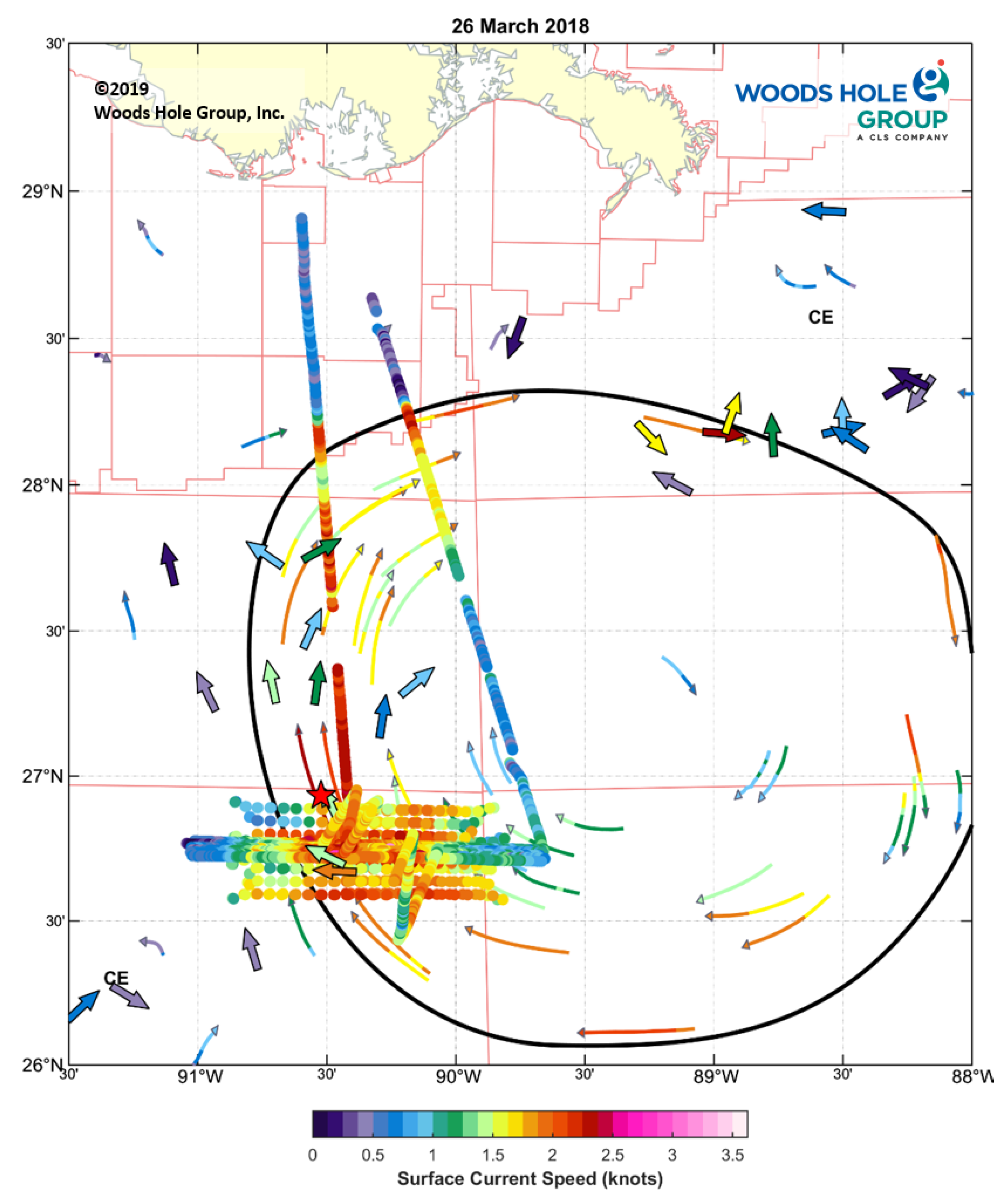
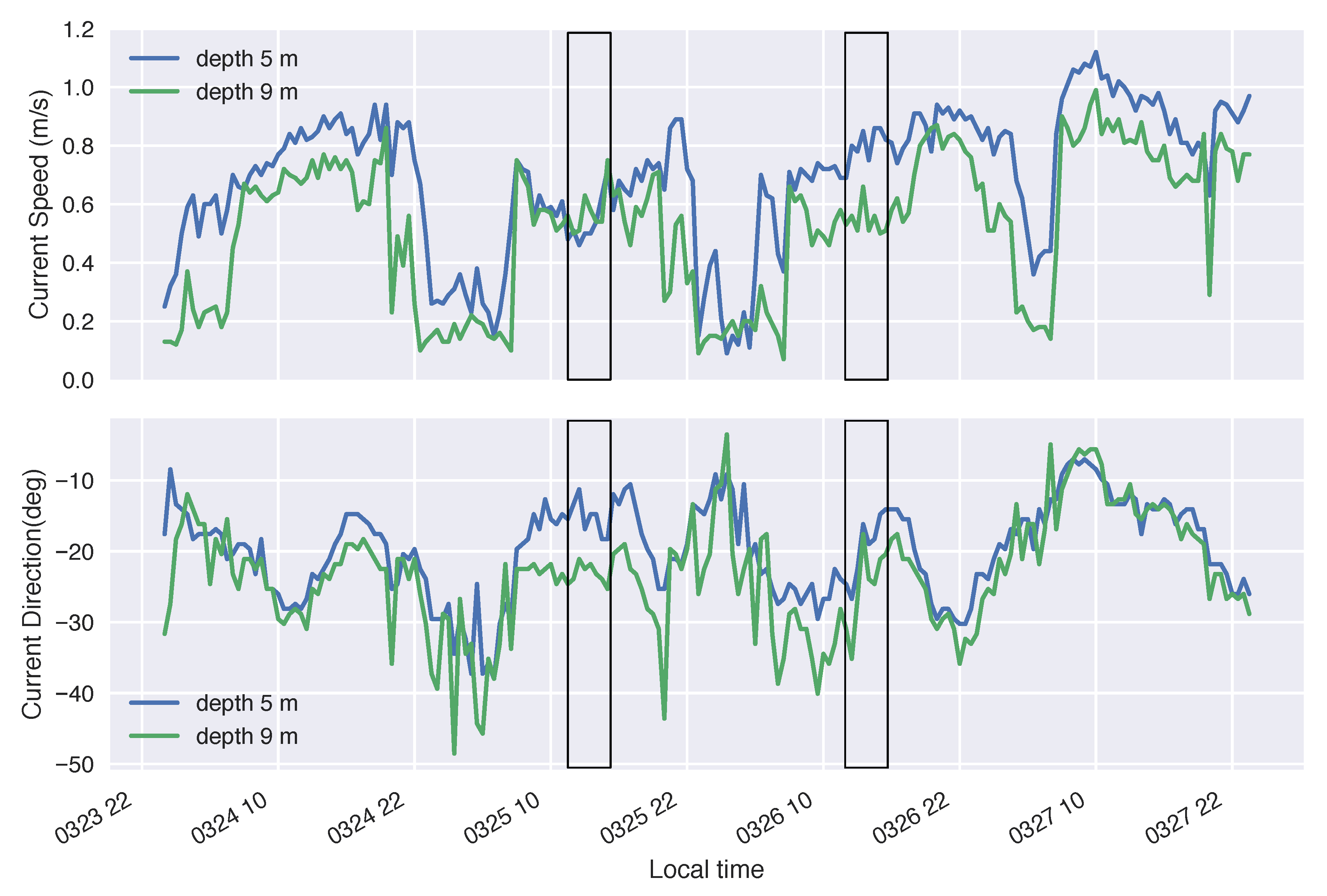
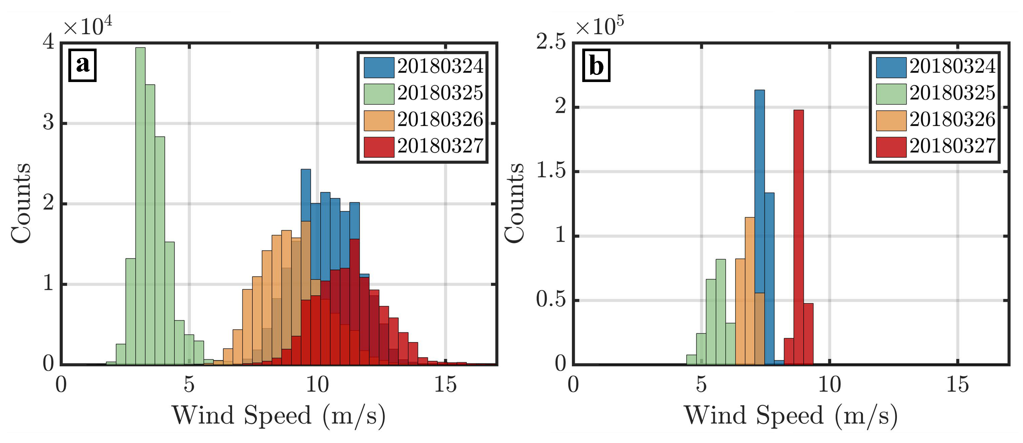
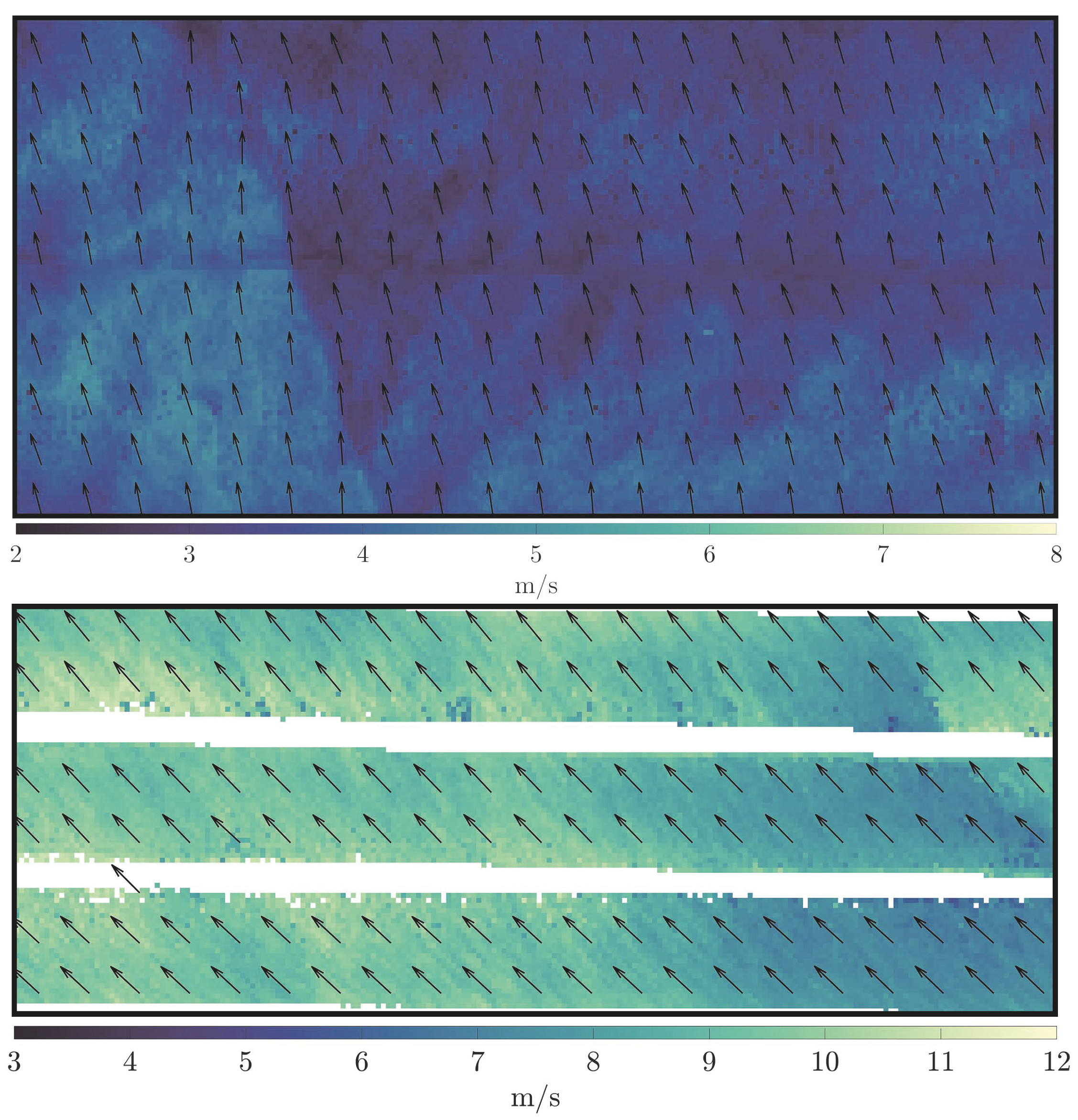
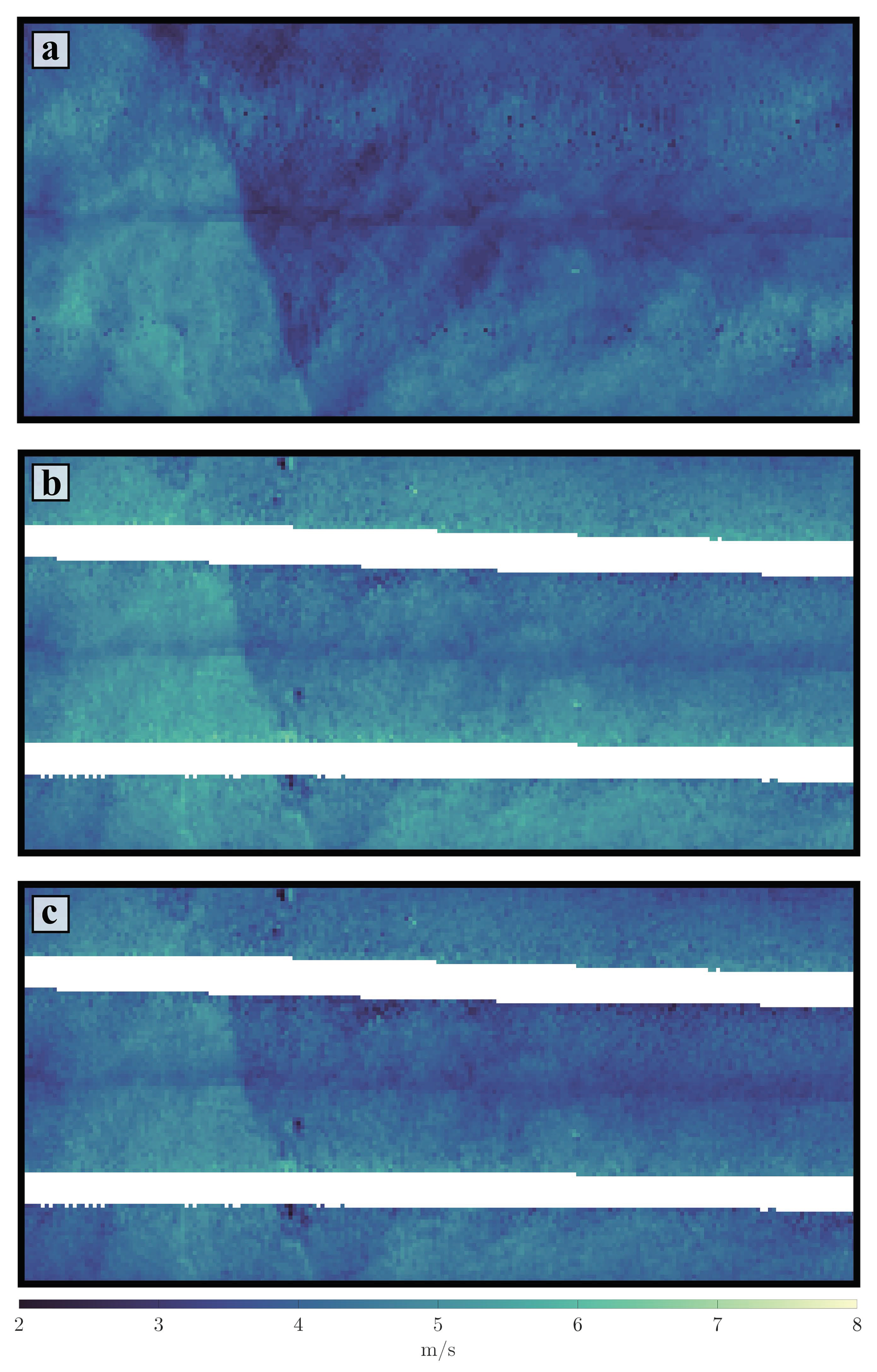
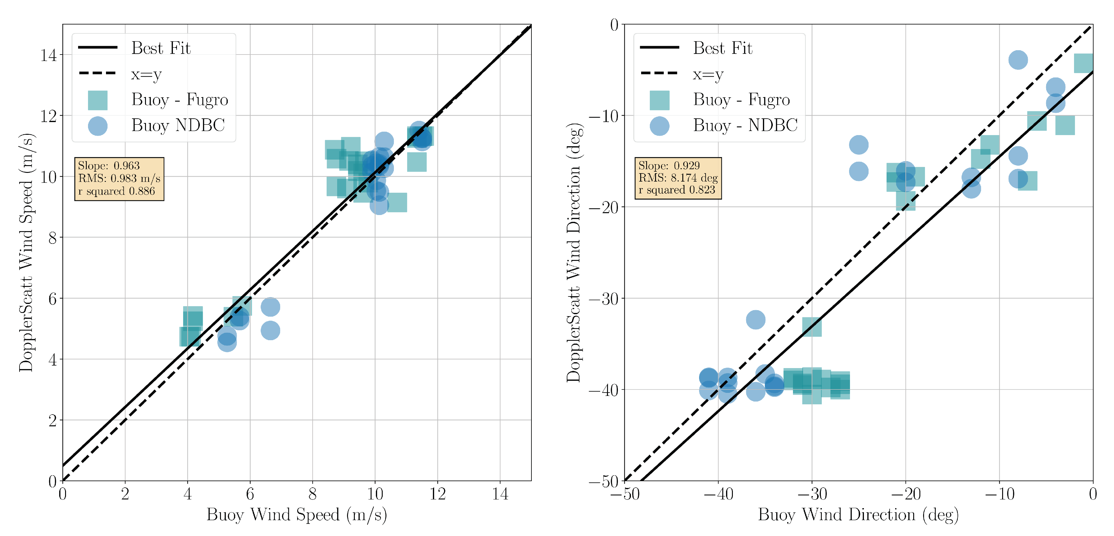
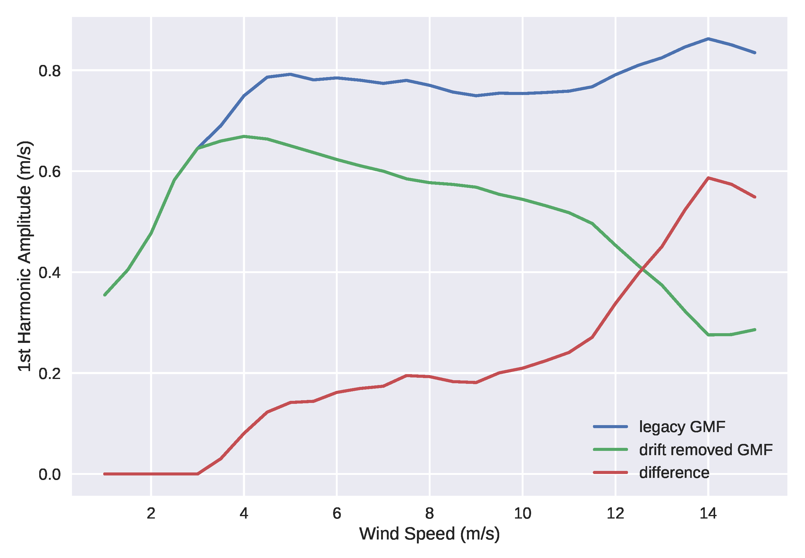
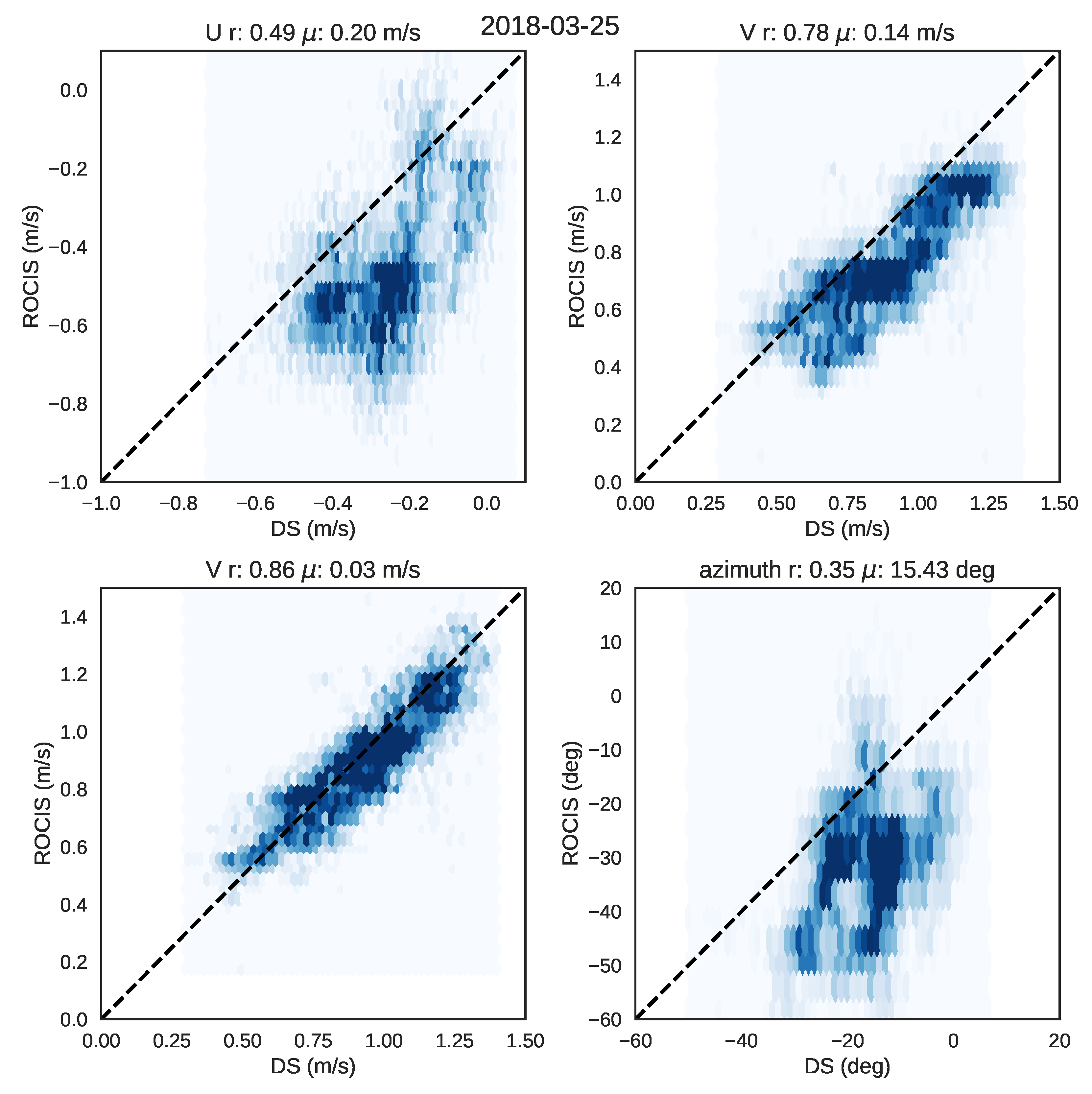
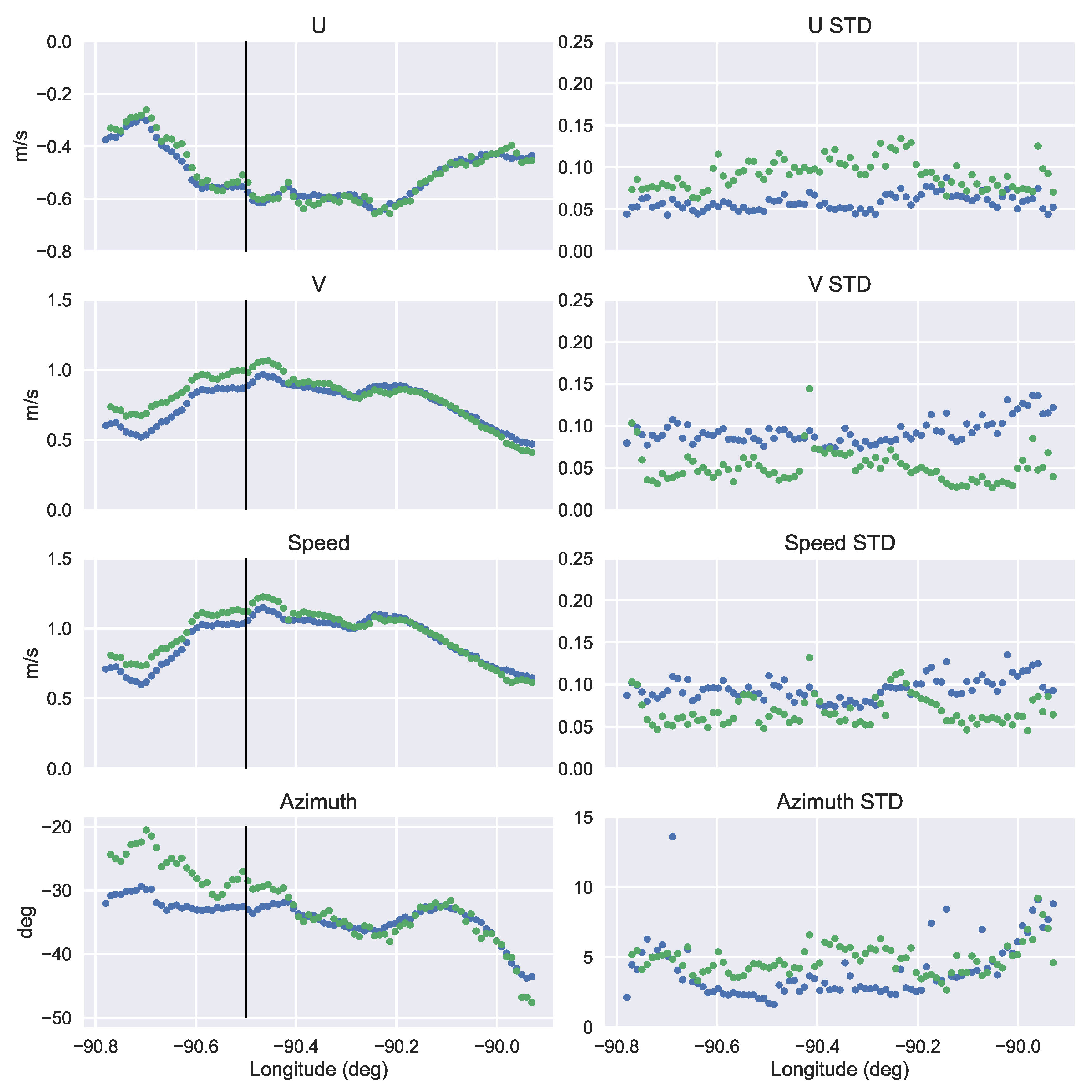
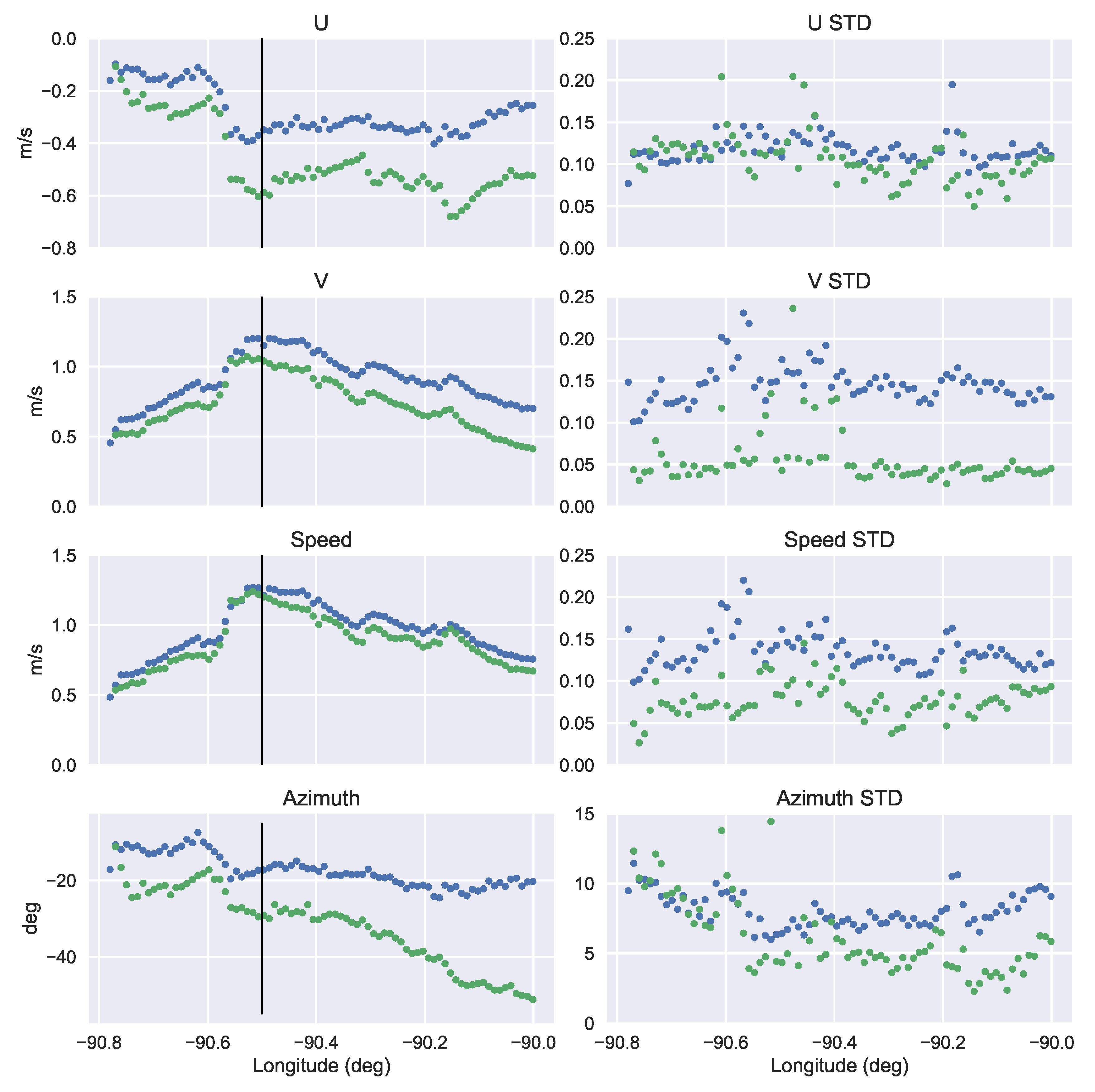
Table 1.
(Top two sub-tables) Wind drift correction as a function of wind speed using all data (first sub-table) and data from the northern swath (second sub-table), which looks into the wind. (bottom two sub-tables) Same as top two subtables, but with the drift velocity parametrized as .
Table 1.
(Top two sub-tables) Wind drift correction as a function of wind speed using all data (first sub-table) and data from the northern swath (second sub-table), which looks into the wind. (bottom two sub-tables) Same as top two subtables, but with the drift velocity parametrized as .
| Wind Speed (m/s) | (deg) | |
|---|---|---|
| All data | ||
| 3 | 9.18 | −114.34 |
| 4 | 5.75 | −97.05 |
| 6 | 3.09 | 7.28 |
| 7 | 3.23 | 17.25 |
| North swath only | ||
| 3 | 5.83 | −111.12 |
| 4 | 2.76 | −68.04 |
| 6 | 4.16 | 24.78 |
| 7 | 3.93 | 29.22 |
| All data, no | ||
| 3 | −5.42 | 0 |
| 4 | −1.31 | 0 |
| 6 | 2.86 | 0 |
| 7 | 2.59 | 0 |
| North swath only, no | ||
| 3 | −3.73 | 0 |
| 4 | 0.45 | 0 |
| 6 | 2.68 | 0 |
| 7 | 2.29 | 0 |
© 2020 by the authors. Licensee MDPI, Basel, Switzerland. This article is an open access article distributed under the terms and conditions of the Creative Commons Attribution (CC BY) license (http://creativecommons.org/licenses/by/4.0/).
Share and Cite
MDPI and ACS Style
Rodríguez, E.; Wineteer, A.; Perkovic-Martin, D.; Gál, T.; Anderson, S.; Zuckerman, S.; Stear, J.; Yang, X. Ka-Band Doppler Scatterometry over a Loop Current Eddy. Remote Sens. 2020, 12, 2388. https://doi.org/10.3390/rs12152388
AMA Style
Rodríguez E, Wineteer A, Perkovic-Martin D, Gál T, Anderson S, Zuckerman S, Stear J, Yang X. Ka-Band Doppler Scatterometry over a Loop Current Eddy. Remote Sensing. 2020; 12(15):2388. https://doi.org/10.3390/rs12152388
Chicago/Turabian StyleRodríguez, Ernesto, Alexander Wineteer, Dragana Perkovic-Martin, Tamás Gál, Steven Anderson, Seth Zuckerman, James Stear, and Xiufeng Yang. 2020. "Ka-Band Doppler Scatterometry over a Loop Current Eddy" Remote Sensing 12, no. 15: 2388. https://doi.org/10.3390/rs12152388
Note that from the first issue of 2016, this journal uses article numbers instead of page numbers. See further details here.