Sharpening the Sentinel-2 10 and 20 m Bands to Planetscope-0 3 m Resolution


1
Center for Global Change and Earth Observations, Michigan State University, East Lansing, MI 48823, USA
2
Department of Geography and Geospatial Sciences, and Geospatial Sciences Center of Excellence, South Dakota State University, Brookings, SD 57007, USA
3
Department of Geography, Environment, and Spatial Sciences, Michigan State University, East Lansing, MI 48824, USA
*
Author to whom correspondence should be addressed.
Remote Sens. 2020, 12(15), 2406; https://doi.org/10.3390/rs12152406
Submission received: 29 June 2020
/
Revised: 19 July 2020
/
Accepted: 25 July 2020
/
Published: 27 July 2020
(This article belongs to the Section Environmental Remote Sensing)
Abstract
:Combination of near daily 3 m red, green, blue, and near infrared (NIR) Planetscope reflectance with lower temporal resolution 10 m and 20 m red, green, blue, NIR, red-edge, and shortwave infrared (SWIR) Sentinel-2 reflectance provides potential for improved global monitoring. Sharpening the Sentinel-2 reflectance with the Planetscope reflectance may enable near-daily 3 m monitoring in the visible, red-edge, NIR, and SWIR. However, there are two major issues, namely the different and spectrally nonoverlapping bands between the two sensors and surface changes that may occur in the period between the different sensor acquisitions. They are examined in this study that considers Sentinel-2 and Planetscope imagery acquired one day apart over three sites where land surface changes due to biomass burning occurred. Two well-established sharpening methods, high pass modulation (HPM) and Model 3 (M3), were used as they are multiresolution analysis methods that preserve the spectral properties of the low spatial resolution Sentinel-2 imagery (that are better radiometrically calibrated than Planetscope) and are relatively computationally efficient so that they can be applied at large scale. The Sentinel-2 point spread function (PSF) needed for the sharpening was derived analytically from published modulation transfer function (MTF) values. Synthetic Planetscope red-edge and SWIR bands were derived by linear regression of the Planetscope visible and NIR bands with the Sentinel-2 red-edge and SWIR bands. The HPM and M3 sharpening results were evaluated visually and quantitatively using the Q2n metric that quantifies spectral and spatial distortion. The HPM and M3 sharpening methods provided visually coherent and spatially detailed visible and NIR wavelength sharpened results with low distortion (Q2n values > 0.91). The sharpened red-edge and SWIR results were also coherent but had greater distortion (Q2n values > 0.76). Detailed examination at locations where surface changes between the Sentinel-2 and the Planetscope acquisitions occurred revealed that the HPM method, unlike the M3 method, could reliably sharpen the bands affected by the change. This is because HPM sharpening uses a per-pixel reflectance ratio in the spatial detail modulation which is relatively stable to reflectance changes. The paper concludes with a discussion of the implications of this research and the recommendation that the HPM sharpening be used considering its better performance when there are surface changes.

1. Introduction
The Sentinel-2A and -2B satellites, launched in 2015 and 2017, respectively, acquire global land surface data at 10 m, 20 m, and 60 m in the visible, near infrared (NIR), and shortwave infrared (SWIR) bands [1]. Each sensor has a 10 day repeat cycle, acquired from a sun synchronous polar orbit, and together they provide globally a median average satellite revisit of 3.7 days [2]. Planetscope data are acquired from a constellation of low cost satellites to provide ~3 m red, green, blue, and NIR data, with a near-daily global coverage [3]. Consequently, there is potential for improved global monitoring using near-daily, 3 m, visible to SWIR data, if the Sentinel-2 and Planetscope data can be combined together.
A number of medium to high resolution sensor fusion approaches exist [4,5]. Several are based on sharpening, whereby coarser spatial resolution band data are sharpened by injecting high frequency spatial details derived by filtering contemporaneous but higher spatial resolution data [6,7]. Typically, sharpening requires multispectral sensor data with a panchromatic band that has lower spectral resolution but higher spatial resolution than the other image bands. When the data from one sensor are used to sharpen the data from another sensor there are additional challenges, particularly if (i) the sensors have different and spectrally nonoverlapping bands, and (ii) if the images are acquired on different dates when the land surface has changed [8,9]. These two issues are the focus of this study, as Planetscope data have no equivalent Sentinel-2 red-edge and SWIR bands, and Planetscope and Sentinel-2 data are often acquired over the same location on different days.
Sharpening methods can be classified broadly into two groups: component substitution and multiresolution analysis [10,11]. Given the global near-daily coverage of Sentinel-2 and Planetscope data, computationally inexpensive sharpening methods are preferable. Previously we sharpened Landsat data using component substitution methods due to their computational efficiency, which make them appropriate for large area application [8,12]. In this study we use two multiresolution analysis sharpening methods that are relatively computationally efficient but cause less spatial distortion than component substitution methods while preserving the spectral properties of the lower resolution imagery [13,14]. This is important as the 10 m and 20 m Sentinel-2 data are systematically calibrated pre and postlaunch [15,16], whereas the Planetscope data have no onboard calibration and so have less reliable calibration [17]. In addition, the different Planetscope sensors can have different spectral response functions and may result in inconsistent reflectance among sensors [18]. A number of multiresolution analysis sharpening methods have been developed, but in this study, we select two that are computationally quite efficient and well established [13,19]. The high pass modulation (HPM) [20,21] and the third modulation method [6], often referred to as model 3 modulation (M3) [13,22], are used.
Sentinel-2 and Planetscope cloud-free data acquired one day apart over three study sites in Zambia and that include land surface changes are considered. The HPM and M3 methods are used to sharpen the 10 m Sentinel-2 visible and NIR bands to 3 m and to sharpen the 20 m Sentinel-2 red-edge, NIR, and SWIR bands to 3 m. As the Planetscope sensors have no red-edge or SWIR bands, synthetic 3 m red-edge and SWIR reflectance, created by regression of the four Planetscope bands with Sentinel-2 red-edge and SWIR 20 m bands, are used in the sharpening process. The sharpening results are assessed by qualitative inspection and quantitative evaluation using the Q2n metric [23] applied for each site and for spatial subsets that contained surface changes between the Sentinel-2 and Planetscope image acquisitions. The paper is structured as follows. First, the satellite data are described, then the image preprocessing (geometric registration and atmospheric correction), followed by the sharpening and evaluation methods, the results, discussion, and a brief conclusion.
2. Data and Study Sites
2.1. Satellite Data Characteristics
The Sentinel-2A and Sentinel-2B satellites, launched by European Space Agency (ESA) in 2015 and 2017, respectively, carry the Multi Spectral Instrument (MSI) sensor that senses a 290-km-wide swath including 10 m and 20 m multispectral bands (Table 1) [1]. The three Sentinel-2 60 m bands are not used as they are designed for cloud screening and atmospheric correction and not for surface monitoring. Sentinel-2 L1C top of atmosphere (TOA) data available from the Copernicus Open Access Hub (https://scihub.copernicus.eu/dhus) were used. The data are ortho-rectified and defined in 109 km × 109 km tiles in the Universal Transverse Mercator (UTM) projection [24]. Nominally, the Sentinel-2 L1C data have a 3% radiometric calibration accuracy [25] and geolocation <12.5 m and band-to-band registration accuracies less than 3 m and 6 m for the 10 m and 20 m bands, respectively [26]. Prior to June 15 2016 [27], the geolocation of Sentinel-2 data was less accurate. Consequently, in this study Sentinel-2 images acquired after this date are used.
Currently, there are about 140 Planetscope sensors operating in low-earth sun-synchronous orbits and, depending on their altitude, acquire 3.7–4.1 m pixel images, which are resampled to 3.0 m for distribution [3,28]. There have been several generations of Planetscope sensor, and in this study, Planetscope-0 sensor data, sometimes referred to as Dove Classic data, which sense blue, green, red, and near infrared (NIR) spectral bands (Table 1), were used. Different Planetscope-0 sensors may have different spectral response functions, and the red, green, and blue bands can spectrally overlap [18]. Their calibration is quantified on orbit by examination of Landsat 8 operational land imager images acquired over pseudo-invariant calibration sites, the moon, and crossover RapidEye images, and is about 5–6% [17]. Their geolocation is typically less than a pixel, with a reported horizontal 4.8 m RMSE [29].
The Planet atmospherically corrected Level 3B surface reflectance product, available to the research team through the NASA Commercial Smallsat Data Acquisition (CSDA) program, was used. The surface reflectance is derived using the 6S radiative transfer code assuming a continental aerosol model [30] and using the spatially and temporally closest available MODIS aerosol optical depth (AOD) data [31]. For brevity, in the rest of the paper we refer to the Planetscope-0 surface reflectance as “Planetscope reflectance”.
2.2. Study Sites and Satellite Data
Study sites where Sentinel-2 and Planetscope-0 cloud-free images, sensed only a day apart, that covered a range of heterogeneous and homogenous areas and that include surface changes between the Sentinel-2 and Planetscope-0 acquisitions were selected. Three study sites in Western Zambia located south of the town of Mongu, near the Zambezi river, in the Northern Kalahari sand basin that is characterized by open Miombo woodland and has near annual fires [32] were selected. The Sentinel-2 and Planetscope-0 data were sensed one day apart (Table 2) and include surface changes with distinct and diffuse changes due to fire that occurred between acquisitions. Three sites defined by 6 × 6 km image subsets were selected for detailed analysis. These sites include woodland and woodland clearing (Site 1, Figure 1), roads and burned areas that occurred between the Sentinel-2 and Planetscope-0 acquisitions (Site 2, Figure 2), and low density settlement and water bodies (Site 3, Figure 3). The selected Sentinel-2 images were acquired by Sentinel-2B over tile 34LGH, and the selected Planetscope-0 images were acquired by Planetscope sensors 103b, 0f28, and 101c.
2.3. Data Preprocessing
There are a number of issues that may need to be considered before the reflectance from different sensors can be used reliably together. These include differences in the sensor (i) spectral band passes, (ii) calibration, (iii) spatial registration, (iv) atmospheric contamination and correction, and (v) bidirectional reflectance effects [16,33,34]. In this study, the first two issues are expected to be handled primarily by the multiresolution analysis sharpening methods. The sensor spectral bandpass differences are accommodated for in the sharpening methodology (Section 3), and as noted above, multiresolution analysis sharpening methods cause less spatial distortion while preserving the spectral properties of the lower resolution Sentinel-2 data that are calibrated. However, some of the Sentinel-2 and Planetscope-0 bands are spectrally quite different, for example, the Sentinel-2 red and green bands are much narrower than for Planetscope-0. Notably, Sentinel-2 has two NIR bands, a 20 nm wide 20 m band and a 115 nm wide 10 m band, and the Planetscope-0 NIR band only marginally overlaps with the 20 m Sentinel-2 NIR band.
The Sentinel-2 and Planetscope-0 data were coregistered using the open-source LSReg v2.0.2 software [27,35] that has been used in a number of recent studies [33,34,36]. Before application of the LSReg software, the four Planetscope-0 bands and the Sentinel-2 10 m NIR band were independently resampled within their own image coordinate systems to 3.333 m by bilinear resampling. The 3.333 m NIR bands for both sensors were then matched using the LSReg software to derive affine mapping transformations. Each band of the Sentinel-2 10 m and 20 m data (Table 1) was reprojected into registration with the Planetscope-0 3.333 m grid using the affine transformation coefficients. The indirect approach was used [37] whereby the location of each Planetscope-0 3.333 m image pixel was mapped into the Sentinel-2 image and then the Sentinel-2 10 m/20 m band values were bilinear resampled to 3.333 m resolution. This procedure was applied for each study site to provide registered Planetscope-0 and Sentinel-2 10 m and 20 m bands defined with 3.333 m pixels. A 3.333 m pixel size was used so that the pixel sizes of the Sentinel-2 10 m and 20 m data were an integer multiple (three and six times, respectively) of the 3.333 m pixel size; this is needed for the sharpening evaluation (Section 3.4).
The Sentinel-2 data were atmospherically corrected to surface reflectance so that they could be compared with the Planetscope-0 Level 3B surface reflectance. The Sen2Cor v2.5.5 atmospheric correction package was run with the default parameter settings [38]. The Sen2Cor surface reflectance accuracy has been validated by comparison with sample ground-based AERONET surface reflectance values with root mean square reflectance errors < 0.013 (visible bands) and < 0.028 (NIR and SWIR bands) [39]. The atmospheric correction accuracy of the Planetscope-0 data is unknown and will depend primarily on the quality and how representative the MODIS AOD data used to derive the surface reflectance are.
The satellite data were not corrected for bidirectional reflectance effects. View zenith bidirectional reflectance effects can be significant across a Sentinel-2 swath and as great as 0.1 (reflectance units 0-1 range) in the SWIR band, about 0.08 in the red-edge and NIR bands, and 0.06 in the visible bands [40,41]. However, the sensor view zenith angles varied by less than half degree across each 6 km × 6 km study area. The Sentinel-2 and Planetscope-0 images were sensed one day apart with overpass time differences (Table 2) <8 min, <4 min, and <50 min for sites 1, 2, 3, that resulted in solar zenith differences of <1.5° for sites 1 and 2 but ~11° for site 3. The solar zenith differences are negligible for sites 1 and 2 but a solar zenith change of the order of 10° has been shown to introduce non-negligible Landsat bidirectional reflectance effects over anisotropic surfaces [42]. The reflectance impact of these sensor view and solar angle variations will vary spatially due to different surface anisotropy across the study sites. We assume that all these differences will be modeled for each pair of Planetscope-0 and Sentinel-2 images by the sharpening process, which incorporates an adaptive modulation of the local high spatial frequency image content (Section 3.2 and Section 3.3).
3. Sharpening Methods
3.1. Overview and Core Processing Calculations
The HPM and M3 multiresolution analysis sharpening methods were used to sharpen the different Sentinel-2 bands to 3.333 m using the Planetscope-0 data. The two sharpening methods are described in Section 3.2 and Section 3.3. For both methods, (i) spatially degraded versions of the 3.333 m Planetscope-0 data degraded to the Sentinel-2 10 m and 20 m resolutions and (ii) synthetic 3.333 m red-edge and SWIR reflectance bands, were needed. These two core processing steps are described below.
3.1.1. Planetscope-0 Spatial Degradation
Spatial degradation of the 3.333 m Planetscope-0 study area data to the Sentinel-2 10 m and 20 m resolutions was undertaken by modeling the smoothing effects of the Sentinel-2 imaging process (sensor optics, analog to digital conversion, and motion blur) described conventionally by the system point spread function (PSF), or the modulation transfer function (MTF), i.e., the magnitude of the Fourier transform of the system PSF [43]. It is well established that if an incorrect PSF is used then sharpened images have reduced quality [7,44]. A 41 × 41 convolution filter with weights that sum to 1.0 was convolved across the Planetscope-0 3.333 m data to degrade each Planetscope-0 band.
where is a filter weight for Sentinel-2 band λ, with i and j ∈ so that i = 0, j = 0 is the center of the 41 × 41 filter, and is defined as:
where is the standard deviation (m−1) of the MTF of the system PSF for Sentinel-2 band and is defined as:
where MTF is the modulation transfer function of the system PSF, f is the spatial frequency (m−1), and is the standard deviation of the MTF (m−1) for Sentinel-2 band λ. We used the published Sentinel-2 MTF values that are defined for the Nyquist frequency [45], i.e., for half of the sample rate, e.g., when f = 1/20 m−1 and f = 1/40 m−1 for the 10 m and the 20 m Sentinel-2 pixels, respectively. We derived analytically from the Sentinel-2B MTF Nyquist frequency values, with values of 0.0318, 0.0313, 0.0305, and 0.0292 for the 10 m blue, green, red, and 115 nm NIR bands, respectively, and values of 0.0173, 0.0166, 0.0168, 0.0163, 0.0137, and 0.0148, for the 20 m three red edge, the 20 nm NIR, and the two SWIR bands, and then from these values we defined as Equation (2). The filter weights in Equation (1) were normalized in the conventional manner, i.e., by multiplying each weight by so that the 41 × 41 filter weights sum to one.
3.1.2. Planetscope-0 synthetic Red-edge and SWIR Band Derivation
As the Planetscope-0 sensors have no equivalent bands to the Sentinel-2 20 m red-edge and SWIR bands (Table 1), synthetic 3.333 m equivalent bands were derived for each study site 3.333 m pixel as:
where is the synthetic Planetscope-0 reflectance at 3.333 m pixel location (i, j) defined for 20 m Sentinel-2 band (red-edge or SWIR, Table 1), , , , and are the Planetscope-0 3.333 m red, green, blue, and NIR reflectance pixel values, and , , , and are weights. The weights were derived by least squares regression of the Sentinel-2 reflectance with respect to the four Planetscope-0 bands spatially degraded to 20 m as:
where is the 20 m Sentinel-2 band (red-edge or SWIR) and , , , and are the spatially degraded Planetscope 20 m red, green, blue, and NIR reflectance values derived as described in Section 3.1.1. The regression was undertaken for each study site considering the 300 × 300 20 m pixels. A linear regression was used in Equation (5) because nonlinear regression and nonparametric models (e.g., random forest regression) showed no improvement over linear models for the prediction of Sentinel-2 red-edge reflectance using Landsat-8 reflectance [46] and we previously found that a linear wavelength dependent interpolation of the red and NIR MODIS BRDF model parameters enabled BRDF normalization of the Sentinel-2 red-edge bands [40].
3.2. High Pass Modulation (HPM) Sharpening
The high pass modulation (HPM) sharpening method was developed originally to sharpen Landsat Thematic Mapper 30 m to SPOT 10 m data [20]. In this study the HPM method was used to sharpen the Sentinel-2 red, green, blue, and NIR bands with the corresponding Planetscope-0 red, green, blue, and NIR bands. In addition, the HPM was modified to sharpen the Sentinel-2 red-edge and SWIR bands.
The 10 m Sentinel-2 red, green, blue, and NIR bands, and the 20 m NIR band, were sharpened to 3.333 m as:
where is the HPM sharpened Sentinel-2 band (red, green, blue, or NIR) reflectance at 3.333 m pixel location (i, j), is the 3.333 m pixel Planetscope-0 band reflectance, d is the appropriate Sentinel-2 10 m or 20 m pixel size for Sentinel-2 band λ (Table 1), >> 3.3 denotes bilinear resampling to 3.333 m, and 3.3 → d denotes spatial degradation from 3.333 m to d m. The product term to the left of in Equation (6) defines the scalar HPM modulation coefficient, which is similar to the Brovey modulation coefficient [47].
The Sentinel-2 20 m red-edge and SWIR bands were sharpened to 3.333 m as:
where is the HPM sharpened Sentinel-2 band (red-edge or SWIR) reflectance at 3.333 m pixel location (i, j), is the 3.333 m synthetic Planetscope band reflectance derived as Equation (4), denotes bilinear resampling to 3.333 m, and 3.3 → 20 denotes spatial degradation from 3.333 m to 20 m.
3.3. Model-3 (M3) Sharpening
The Model 3 (M3) sharpening method was originally developed to sharpen SPOT 20 m data to 10 m [6] and has been refined in a variety of ways that are often computationally intensive [22,48,49]. In this study, the original M3 method was used.
The Sentinel-2 10 m red, green, blue, and NIR bands, and the 20 m NIR band, were sharpened to 3.333 m as:
where is the M3 sharpened Sentinel-2 band λ (red, green, blue, or NIR) reflectance at 3.333 m pixel location (i, j), d is the appropriate Sentinel-2 10 m or 20 m pixel size for Sentinel-2 band λ (Table 1), is the Sentinel-2 λ band reflectance, and is the 3.333 m pixel Planetscope-0 λ band reflectance. As before, denotes bilinear resampling to 3.333 m, and 3.3 → d denotes spatial degradation from 3.333 m to d resolution.
The term in Equation (8) is the scalar M3 modulation coefficient that is defined from the ratio of the reflectance covariance in an m × m window centered on 3.333 m pixel location (i, j) defined as:
where is the covariance of terms and where and denote the m2 3.333 m Sentinel-2 band reflectance values and the m2 3.333 m Planetscope-0 band reflectance values, respectively, in the square m × m window centered on (i, j). As before, denotes a d resolution pixel bilinear resampled to 3.333 m, and 3.3 → d denotes spatial degradation from 3.333 m to d resolution, with d set as the appropriate Sentinel-2 10 m or 20 m pixel size for Sentinel-2 band (Table 1). The scalar modulation coefficient is similar to the Gram Schmidt modulation term used in the component substitution sharpening method [50]. In this study, as suggested in Zhang and Roy [12], an m = 13 window size was used, i.e., each window used in Equation (9) was defined by a square neighborhood of 169 pixels.
The Sentinel-2 20 m red-edge and SWIR bands was sharpened to 3.333 m as:
where is the M3 sharpened Sentinel-2 red-edge or SWIR reflectance at 3.333 m pixel location (i,j), is the 20 m pixel Sentinel-2 band reflectance, is the M3 scalar modulation coefficient defined as Equation (9), and is the 3.333 m synthetic Planetscope-0 band reflectance derived as Equation (4). As before, denotes bilinear resampling to 3.333 m, and 3.3 → d denotes spatial degradation from 3.333 m to d resolution.
3.4. Sharpening Evaluation
The sharpening results were first evaluated by visual inspection of the 6 × 6 km sharpened study site images and by examination of 800 × 800 m spatial subsets located where surface changes occurred in the one day acquisition difference between the Sentinel-2 and Planetscope-0 imagery.
A conventional quantitative evaluation was also undertaken. Specifically, the 10 m Sentinel-2 and 3.333 m Planetscope-0 bands were spatially degraded by a factor of three to 30 m and 10 m, respectively, and the 20 m Sentinel-2 and the 3.333 m Planetscope-0 bands were degraded by a factor of six to 120 m and 20 m, respectively. In this way the scale differences between the Sentinel-2 and the Planetscope-0 bands were preserved and the spatially degraded Sentinel-2 and Planetscope-0 data have integer pixel sizes. The spatial degradation was undertaken following the method described in Section 3.1.1. Thus, the Planetscope-0 degradation was undertaken using the Sentinel-2 system PSF as the Planetscope-0 PSF is unavailable and because the system PSF defined by Equation (1) has a Gaussian form, which is the usual form used when the system PSF is unspecified [51,52,53,54]. The spatially degraded Sentinel-2 bands were then sharpened to their original resolutions using the HPM and M3 methods and the sharpened results were compared with the original resolution imagery using the metric. The metric was used as it quantifies spectral and spatial distortions between n band images as a single value falling between 0 and 1 (where higher values mean less spectral and spatial distortion) [23]. Specifically, the metric was calculated by dividing the image area into nonoverlapping adjacent square windows, each composed of N × N pixels. For each window the metric was derived [23,55] as
where is the covariance of reference image and test image over the N × N window area, and are the variances, and and are the mean values, of reference image and test image , respectively. The metric was developed based on the Universal Image Quality Index (UIQ) metric for monochrome imagery [55] by treating multiple band pixel spectra as hypercomplex numbers [23,56]. The hypercomplex number is an extension of the two-dimensional (2-D) complex numbers to 4-D quaternions, 8-D octonions, and to 2n-D for any band number [23]. The first term in Equation (11) is similar to the correlation coefficient and means that the metric captures differences in the spatial structure between images that are not captured by simpler difference based metrics such as the bias, root-mean-squared difference, or signal-to-noise ratio [55].
The values were derived considering the different Sentinel-2 spectral bands individually (n = 1) and considering the 10 m bands (n = 4) and the 20 m bands (n = 6) together. The values were derived for nonoverlapping adjacent 8 × 8 (i.e., N = 8) pixel windows across each study site (75 × 75 and 38 × 38 values for the 10 m and 20 m bands, respectively) and also across each spatial subset (10 × 10 and 5 × 5 values for 10 m and 20 m bands, respectively). The mean value was used to summarize the different values.
4. Results
4.1. Visual Evaluation
Figure 1, Figure 2 and Figure 3 illustrate the three study sites and show the Sentinel-2 true color surface reflectance bilinear resampled from the original 10 m resolution to 3.333 m (a), the Planetscope-0 3.333 m true color surface reflectance (b), and the HPM (c) and M3 (d) sharpened Sentinel-2 3.333 m true color surface reflectance images. The study sites contain a variety of high spatial frequency features and high contrast edges associated with fields (Figure 1), roads and buildings (Figure 2 and Figure 3), and the edges between highly reflective Kalahari sand and burned vegetation areas (Figure 3). Even at this scale (6 × 6 km), the richer spatial detail provided by the Planetscope-0 imagery (b) compared to the Sentinel-2 imagery (a) is evident.
Figure 4, Figure 5 and Figure 6 illustrate, for the three study sites, false color surface reflectance images showing NIR, red-edge, and SWIR results. At these longer wavelengths burned areas are apparent, particularly across the central portion of site 2 (Figure 5). Figure 4, Figure 5 and Figure 6 show the Sentinel-2 NIR (855–875 nm), red-edge (773–793 nm), and SWIR (1565–1655 nm) 20 m reflectance bilinear resampled to 3.333 m (a), the Planetscope-0 NIR 3.333 m band and the synthetic red-edge (773–793 nm) and SWIR (1565–1655 nm) 3.333 m bands derived as Equation (4) (b), and the results of HPM (c) and M3 (d) sharpening of the 20 m Sentinel-2 false color surface reflectance bands to 3.333 m. Discrete objects such as trees in Figure 4 and buildings in Figure 6 and the edges of roads and burned areas in Figure 5 are visually more discernable in the sharpened Sentinel-2 3.333 m imagery than in the bilinear resampled imagery.
In general, the visual improvement of the sharpened Sentinel-2 images compared to the bilinear resampled Sentinel-2 images is more evident in the 20 m to 3.333 m sharpening (Figure 4, Figure 5 and Figure 6) than in the 10 m to 3.333 m sharpening (Figure 1, Figure 2 and Figure 3). There are no apparent ringing or aliasing effects in the HPM and M3 sharpened results indicating that the spatial degradation appropriately modeled the Sentinel-2 band specific system PSF [7,44]. However, at this spatial resolution, there are no significant apparent differences between the HPM and M3 sharpening results, for both the true color and false color results, indicating qualitatively that both sharpening methods work well.
4.2. Visual Evaluation of Spatial Subsets Containing Surface Change
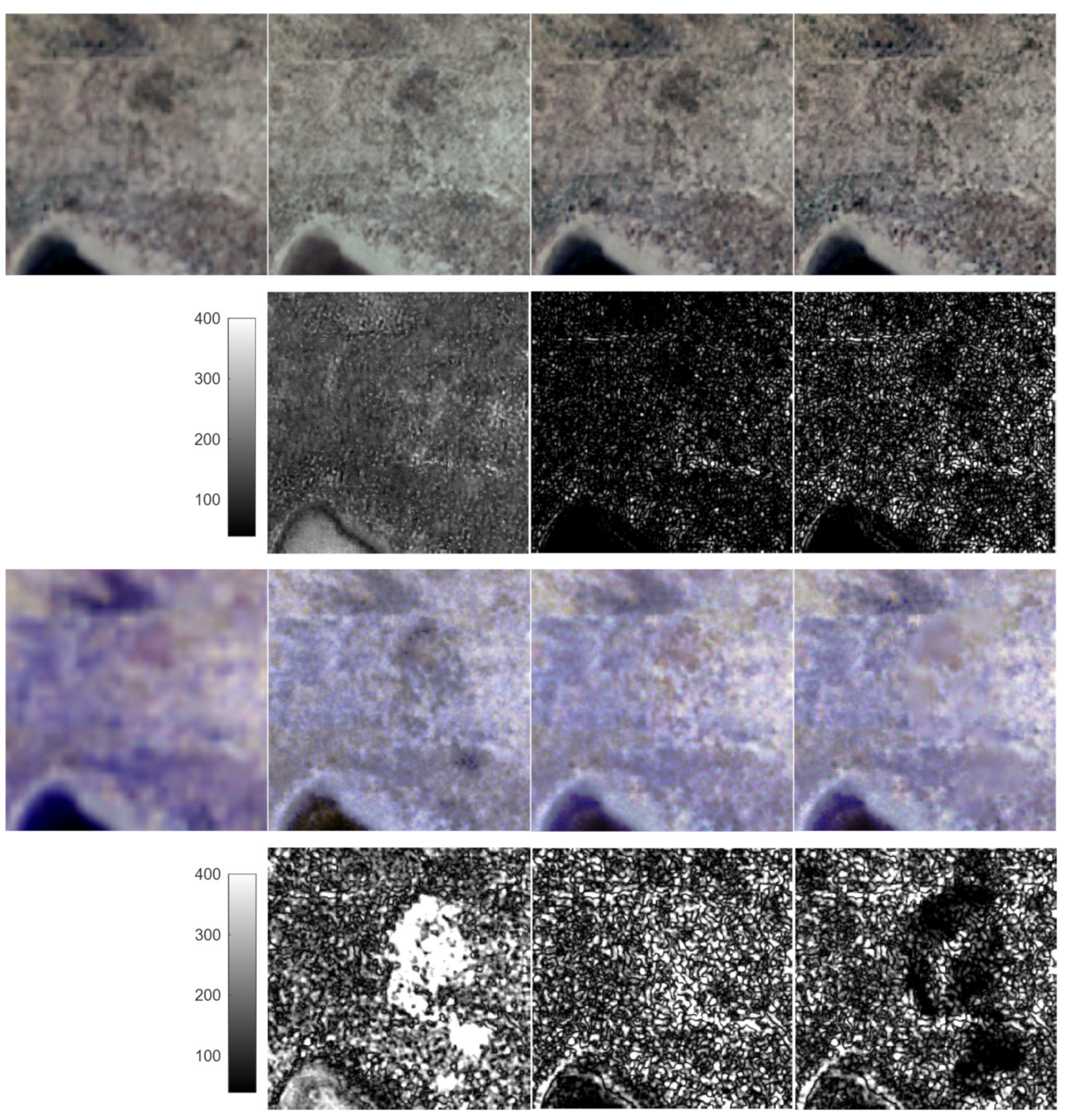
Figure 7, Figure 8 and Figure 9 show detailed 800 × 800 m subsets, composed of 240 × 240 3.333 m pixels, extracted from the three study sites. The figure columns show from left to right: Sentinel-2 surface reflectance bilinear resampled to 3.333 m, Planetscope-0 3.333 m surface reflectance, and the HPM and M3 sharpened 3.333 m surface reflectance. In each figure there are four rows. The first and third rows show subsets of the true color (Figure 1, Figure 2 and Figure 3) and the false color (Figure 4, Figure 5 and Figure 6) surface reflectance, respectively. The second and fourth rows (greyscale figures) shows the difference between the Sentinel-2 bilinear resampled results and each of the results shown in the other three columns. The subsets include surface changes that occurred in one day between the Sentinel-2 and Planetscope-0 acquisitions. The surface changes are due to biomass burning that reduce reflectance at most wavelengths and are most apparent in Sentinel-2 imagery in the NIR, red-edge, and SWIR bands [57] and so are most evident in the illustrated false color results. The difference images show the root mean square difference (RMSD) between the Sentinel-2 bilinear resampled reflectance () and the Planetscope-0, HPM sharpened, and M3 sharpened, reflectance (), derived at each 3.333 m pixel as . As expected, greater RMSD values occur between the Sentinel-2 bilinear resampled reflectance and the Planetscope-0 data along high contrast edges and where surface changes occurred between the sensor acquisitions. In general, the HPM and M3 sharpened results have lower RMSD values than the Planetscope-0 data, indicating the efficacy of the sharpening algorithms.
The unchanged areas within the subsets have more apparent spatial detail in the sharpened results (last two columns) than the bilinear resampled Sentinel-2 reflectance (first column). As for the full study site images, this is particularly apparent for the false color bands. However, differences between the two sharpening methods are not particularly evident. In general, in the unchanged areas, the true color HPM RMSD values (2nd row, 3rd column) are lower than the M3 RMSD values (2nd row, 4th column), but this pattern is less apparent for the false color RMSD results (4th row).
In the changed areas, the two sharpening methods perform quite differently. The M3 method did not reliably sharpen the Sentinel-2 reflectance (4th column) where the changes occurred, resulting in blurred sharpened reflectance and low RMSD values relative to the bilinear resampled Sentinel-2 data that are also blurred. In contrast, the HPM method (3rd column) provides visually more spectrally and spatially coherent results. This difference is most pronounced in the false color reflectance bands, where the changes have more contrast with the surrounding unchanged Planetscope-0 pixels, particularly in Figure 7 and Figure 8 where the changes are more distinct than in Figure 9.
4.3. Quantitative Evaluation
4.3.1. Quantitative Study Site Evaluation
Table 3 summarizes the results for the three study sites considering the four 10 m sharpened Sentinel-2 surface reflectance bands (red, green, blue, and the 115 nm wide NIR band) together, and Table 4 summarizes the results for each band independently. In all cases, the HPM and M3 sharpened reflectance have low spectral and spatial distortion ( values > 0.91) and less distortion than the bilinear resampled Sentinel-2 reflectance ( values ranging from 0.51 to 0.63). For each study site and for each sharpening method, the greatest 10 m band distortions (lowest values) are for the blue band (Table 4).
Table 5 and Table 6 summarize the same results as for Table 3 and Table 4 but considering the six 20 m sharpened bands (the three red-edge, the 20 nm wide NIR, and the two SWIR bands). Again, in all cases, the HPM and M3 sharpened 20 m reflectance have less distortion ( values > 0.76) than the bilinear resampled Sentinel-2 20 m reflectance ( values ranging from 0.23 to 0.34). Notably, the values considering all the 20 m bands together (Table 5) are lower than when considering all the 10 m bands together (Table 3). Considering the individual 20 m band results (Table 6), the shortest wavelength red-edge band (697–713 nm) has the highest values (i.e., the least distortion). Notably, the Sentinel-2 115 nm wide NIR band always has higher values than the 20 nm wide NIR band. This is likely because the Sentinel-2 115 nm wide NIR band overlaps spectrally with the Planetscope-0 NIR band but the Sentinel-2 20 nm wide NIR band does not overlap with the Planetscope-0 NIR band (Table 1).
In Table 3, Table 4, Table 5 and Table 6, the highest values for each table row are highlighted. If the absolute difference between the two sharpening methods (last columns) are within two decimal places, we assume that the values are not meaningfully different. No distinct pattern of difference between the two sharpening methods is apparent. Considering all the 10 m bands together (Table 3), the two methods are similar but with less distortion provided by M3 at site 1. Considering all the 20 m bands together (Table 5) the two methods are similar but with less distortion provided by M3 at site 3 and less distortion provided by HPM at site 2.
4.3.2. Quantitative Evaluation for the Spatial Subsets Containing Surface Change
Table 7, Table 8, Table 9 and Table 10 follow the same order as Table 3, Table 4, Table 5 and Table 6 but show the values for the three subsets illustrated in Figure 7, Figure 8 and Figure 9. As for the full image results, in all cases the HPM and M3 sharpened reflectance in the subsets have low spectral and spatial distortion ( values > 0.87 for the 10 m bands and > 0.70 for the 20 m bands) and less distortion than the bilinear resampled Sentinel-2 reflectance ( values ranging from 0.55 to 0.63 for the 10 m bands and from 0.15 to 0.43 for the 20 m bands). We note that the spatial subset areas are ~98% smaller than the full image areas and are located where surface changes due to biomass burning occurred between the Sentinel-2 and the Planetscope-0 acquisitions. Therefore it is not meaningful to compare the magnitude of the subset values with the full image values that are summarized in Table 3, Table 4, Table 5 and Table 6. However, the relative patterns among bands and sites is of interest and allows us to examine sharpening algorithm sensitivity to surface change.
As before, for the full image results, considering all the 10 m bands together (Table 7) the two sharpening methods perform similarly but with less distortion provided by M3 at site 1. No distinct pattern of difference between the two sharpening methods is apparent considering the individual 10 m bands (Table 8). However, in contrast to the full image results, both sharpening methods performed most poorly for the 115 nm wide 10 m NIR band (Table 8) rather than for the blue band (Table 4).
Considering all the 20 m bands together (Table 9), less distortion is provided by M3 at site 3 (as for the full image, Table 5) but also at site 2, and less distortion is provided by HPM at site 1. However, for the individual 20 m bands, unlike for the full image results (Table 6), the HPM sharpening performed better than M3 for the majority of the bands and sites. Indeed, the M3 method only performed better than HPM for the 1565–1655 nm SWIR band at sites 2 and 3 and for the 2100-2280 nm SWIR band at site 3.
5. Discussion
In this study, Planetscope-0 and Sentinel-2 data were used that have different sensor design and capabilities with differences in the sensor spectral band passes, calibration, geolocation, atmospheric contamination due to overpass time differences, and bidirectional reflectance effects due to surface reflectance anisotropy and the different sensor view and solar geometries. We assumed that the first two issues were accommodated for by the sharpening process, which incorporates, for both the HPM and M3 methods, an adaptive modulation of the local high frequency spatial details. Furthermore, the sharpening methods use multiresolution analysis approaches, which is helpful because they introduce less spatial distortion than component substitution sharpening methods while preserving the spectral properties of the Sentinel-2 imagery. This is important as Sentinel-2 data have more reliable calibration than Planetscope-0 data. The LSReg algorithm used for the coregistration of Sentinel-2 and Planetscope-0 data had subpixel accuracy, which we believe is adequate for image sharpening. The atmospheric correction of the Sentinel-2 and Planetscope-0 data used different radiative transfer codes (6S and Sen2Cor for the Planetscope-0 and Sentinel-2 data, respectively) and different aerosol sources (derived from MODIS and from Sentinel-2 for the Planetscope-0 and Sentinel-2 correction, respectively). The Planetscope-0 atmospheric correction is likely to be less reliable since the MODIS AOD data were acquired at different times from the Planetscope-0 image acquisitions and because fires in the southern Africa can generate dynamic aerosols [58], which may be different in the one day difference between the Planetscope-0 and Sentinel-2 image acquisitions. The degree to which these potential between-sensor atmospheric correction differences affected the sharpening results is unknown. Sensor and solar geometry variations induce BRDF effects that were not corrected for in this study. The view zenith variations were less than half a degree across the 6 km × 6 km study sites. The solar zenith differences were, however, non-negligible, in particular over study site 3 (~11° difference), due to over pass time difference between Sentinel-2 and Planetscopes-0 satellites. We assumed that the reflectance variations caused by different sensor viewing and solar geometries was handled in the sharpening process, which incorporates, for both the HPM and M3 methods, an adaptive modulation of the local high frequency spatial detail. Future research to examine the sharpening impact of differences in the sensor and solar angles is recommended. This research should consider images acquired over a range of view and solar geometries, over a range of surfaces with different surface reflectance anisotropy, including different vegetation canopy architectures and shadow distributions that can be particularly evident in high spatial resolution imagery.
Despite the above differences between the sensed Sentinel-2 and Planetscope-0 data, the HPM and M3 approaches achieved favorable sharpening results with less spatial and spectral distortions than conventional bilinear resampling. Objects in the HPM and M3 sharpened imagery had sharper boundaries and exhibited finer spatial detail than in the bilinear resampled imagery. This was expected and was because the sharpening process injects spatial details from the Planetscope-0 imagery into the coarser spatial resolution Sentinel-2 imagery. In contrast, bilinear resampling smooths the imagery by interpolating reflectance values from four neighboring pixels [59,60].
The Sentinel-2 10 m red, green, blue, and 115 nm NIR spectral bands were sharpened using the approximately corresponding Planetscope-0 red, green, blue, and NIR spectral bands, respectively. The sharpened reflectance had high (i.e., low distortion) values > 0.91 for the three study sites considering all the 10 m bands together and individually. The greatest distortion was found for the blue band (Table 4). This is likely because the shortest wavelength blue band is highly sensitive to aerosols and is the least reliably atmospherically corrected reflective wavelength [39,61] and, as noted above, because the one day acquisition difference means that the Planetscope-0 and Sentinel-2 images may have been affected by different aerosol conditions. No distinct pattern of difference between the two sharpening methods was apparent. Considering all the 10 m bands together in the whole study sites (Table 3), the HPM and M3 methods were broadly similar.
The Sentinel-2 20 m NIR band (20 nm wide) was sharpened using the Planetscope-0 NIR band and the Sentinel-2 20 m red-edge and SWIR bands were sharpened using synthetic red-edge and SWIR bands derived from the Planetscope-0 red, green, blue, and NIR band reflectance values. The values considering all the 20 m bands together were lower (values > 0.76) than those considering all the 10 m bands together. This is because the 10 m band sharpening has a resolution ratio of 3 to the Planetscope-0 reflectance rather than 6 between the 20 m Sentinel-2 and Planetscope-0 reflectance. In addition, there are no Planetscope-0 red-edge and SWIR bands and so synthetic red-edge and SWIR bands were used for the sharpening. Notably, the shortest Sentinel-2 red-edge wavelength band (697–713 nm) had the least distortion (greatest values in Table 6) among all the 20 m bands—likely because it is spectrally close to the Planetscope-0 red band (590–670 nm) that was used for the synthetization of the red-edge band (697–713 nm) (Equation (4)). No distinct pattern of difference between the two sharpening methods was apparent. Considering all the 20 m bands together (Table 5), the two methods were broadly similar.
Sharpening using different sensors will be less reliable if the images are acquired at different times or dates and the surface has changed. This was examined specifically in this paper in detail at three spatial subsets. The M3 method could not reliably sharpen the Sentinel-2 reflectance where surface changes occurred and resulted in blurred reflectance. This is because the M3 sharpening modulation coefficient values (Equation (9)) were low in the surface change areas as the values were derived from the covariance between the two images acquired on different days. Consequently, there were few spatial details injected into the Sentinel-2 imagery and the sharpened image appeared blurred. The HPM method generally did not have this issue and could sharpen the Sentinel-2 bands affected by surface changes. The values of the HPM sharpened surface change results were greater than those of M3 for the majority of the bands and sites. Furthermore, the HPM is computationally much faster than the M3 since the HPM modulation coefficient is derived using a simple ratio calculation (middle part of the Equation (6)), while the M3 modulation coefficient is derived using two covariance calculations and one ratio calculation (Equation (9)). Future research examining other types of surface changes is recommended. We note that sharpening will not be reliable if the sensor imagery are cloudy as typically clouds are spectrally very different to surface conditions. In addition, consideration of Sentinel-2 sharpening using Planetscope imagery acquired with different temporal separations is merited, particularly for separations greater than one day that is likely to occur in persistently cloudy regions.
Currently, there are three generations of Planetscope sensors on orbit (Planetscope-0, -1, and -2) with different characteristics (https://developers.planet.com/docs/data/sensors/). In this study, the first generation Planetscope-0 data were used. Due to the spectral band differences among the Planetscope sensors, the HPM and M3 sharpening methods may perform differently for the Planetscope-1 and Planetscope-2 sensors. For example, the most recent Planetscope-2 sensors have a red-edge band and spectral response functions that closely match the visible, red-edge, and NIR Sentinel-2 bands. Future research to investigate the effectiveness of the HPM and M3 sharpening for the later generation Planetscope sensors is merited.
The PSFs used in this study were derived analytically for each Sentinel-2 10 m and 20 m spectral band from published modulation transfer function (MTF) values [45]. The PSFs were implemented using a spatial domain convolution kernel that can be used for other Sentinel-2 degradation studies and for development of other sharpening algorithms. Because the PSF for each band of the Planetscope-0 sensor are not publicly available, the Sentinel-2 PSF was used in this study to degrade the Planetscope-0 data in the sharpening algorithm evaluation. The impact of this substitution is unknown and a publicly available documentation of the PSFs for each of the Planetscope bands would be helpful.
In the last two decades, algorithms to blend MODIS and Landsat reflectance have been developed to generate synthetic daily Landsat 30 m data [4,62,63,64] and more recently to generate synthetic daily Landsat reflectance without using other satellite data [65,66]. With the availability of commercial high resolution time series there is now considerable interest in combining the data with medium resolution satellite time series for improved terrestrial monitoring. For example, recently, Houborg and McCabe [18] developed an algorithm to adjust 3 m Planetscope visible and NIR reflectance time series to be more consistent with contemporaneous Landsat-8 30 m visible and NIR reflectance. This paper indicates that it is feasible to generate 3 m visible, red-edge, NIR, and SWIR reflectance on days where there are Sentinel-2 observations and where there are spatially overlapping Planetscope data. This approach could be extended to Landast-8 and Sentinel-2 time series and for large area application and is the subject of future research.
6. Conclusions
Sentinel-2 10 m and 20 m imagery were sharpened to Planetscope-0 3 m resolution using two well-established sharpening methods: high pass modulation (HPM) and Model 3 (M3). The methods were demonstrated and evaluated using Sentinel-2 and Planetscope-0 imagery acquired one day apart over three sites in Zambia, which included surface changes due to biomass burning.
Visual and quantitative results demonstrated that:
- (1)
- the HPM and M3 approaches introduced less spatial and spectral distortion in the sharpened Sentinel-2 visible, red-edge, NIR, and SWIR 10 m and 20 m bands relative to conventional Sentinel-2 bilinear resampling; and, over surfaces with no change between the Sentinel-2 and Planetscope-0 acquisitions, the two sharpening methods produced similar results;
- (2)
- the HPM and M3 sharpened Sentinel-2 20 m red-edge and SWIR bands were visually coherent but had more spatial and spectral distortion ( values > 0.76) than the sharpened Sentinel-2 10 m visible and 115 nm NIR bands ( values > 0.91);
- (3)
- the HPM method could sharpen the Sentinel-2 bands affected by surface changes whereas the M3 method generally could not;
- (4)
- the HPM method is recommended for Planetscope-0 sharpening of Sentinel-2 data.
Author Contributions
Conceptualization, Z.L., D.P.R., and H.K.Z.; methodology, H.K.Z. and D.P.R.; software, H.K.Z., Z.L., L.Y., H.H. validation, Z.L.; formal analysis, Z.L.; writing-original draft preparation, D.P.R., Z.L.; writing-review and editing, D.P.R. and H.K.Z., Z.L.; visualization, Z.L.; funding acquisition, D.P.R. All authors have read and agreed to the published version of the manuscript.
Funding
This research was funded by the NASA Commercial Smallsat Data Acquisition (CSDA) program and by the NASA Land Cover/Land Use Change Multi-Source Land Imaging Science Program Grant NNX15AK94G.
Acknowledgments
We thank the management and staff of the ESA and Copernicus programs, and PLANET, for the free provision of the satellite data used in this research.
Conflicts of Interest
The authors declare no conflict of interest.
References
- Drusch, M.; Del Bello, U.; Carlier, S.; Colin, O.; Fernandez, V.; Gascon, F.; Hoersch, B.; Isola, C.; Laberinti, P.; Martimort, P.; et al. Sentinel-2: ESA′s optical high-resolution mission for GMES operational services. Remote Sens. Environ. 2012, 120, 25–36. [Google Scholar] [CrossRef]
- Li, J.; Roy, D.P. A global analysis of Sentinel-2A, Sentinel-2B and Landsat-8 data revisit intervals and implications for terrestrial monitoring. Remote Sens. 2017, 9, 902. [Google Scholar]
- Planet Team. Planet Imagery Product Specifications. Available online: https://www.planet.com/products/ (accessed on 9 March 2020).
- Gao, F.; Masek, J.; Schwaller, M.; Hall, F. On the blending of the Landsat and MODIS surface reflectance: Predicting daily Landsat surface reflectance. IEEE Trans. Geosci. Remote Sens. 2006, 44, 2207–2218. [Google Scholar]
- Li, W.; Jiang, J.; Guo, T.; Zhou, M.; Tang, Y.; Wang, Y.; Zhang, Y.; Cheng, T.; Zhu, Y.; Cao, W.; et al. Generating Red-Edge Images at 3 M Spatial Resolution by Fusing Sentinel-2 and Planet Satellite Products. Remote Sens. 2019, 11, 1422. [Google Scholar] [CrossRef] [Green Version]
- Ranchin, T.; Wald, L. Fusion of high spatial and spectral resolution images: The ARSIS concept and its implementation. Photogramm. Eng. Remote Sens. 2000, 66, 49–61. [Google Scholar]
- Aiazzi, B.; Alparone, L.; Baronti, S.; Garzelli, A.; Selva, M. MTF-tailored multiscale fusion of high-resolution MS and Pan imagery. Photogramm. Eng. Remote Sens. 2006, 72, 591–596. [Google Scholar] [CrossRef]
- Li, Z.; Zhang, H.K.; Roy, D.P.; Yan, L.; Huang, H.; Li, J. Landsat 15-m panchromatic-assisted downscaling (LPAD) of the 30-m reflective wavelength bands to Sentinel-2 20-m resolution. Remote Sens. 2017, 9, 755. [Google Scholar]
- Wang, Q.; Blackburn, G.A.; Onojeghuo, A.O.; Dash, J.; Zhou, L.; Zhang, Y.; Atkinson, P.M. Fusion of Landsat 8 OLI and Sentinel-2 MSI Data. IEEE Trans. Geosci. Remote Sens. 2017, 55, 3885–3899. [Google Scholar] [CrossRef] [Green Version]
- Thomas, C.; Ranchin, T.; Wald, L.; Chanussot, J. Synthesis of multispectral images to high spatial resolution: A critical review of fusion methods based on remote sensing physics. IEEE Trans. Geosci. Remote Sens. 2008, 46, 1301–1312. [Google Scholar] [CrossRef] [Green Version]
- Aiazzi, B.; Baronti, S.; Lotti, F.; Selva, M. A comparison between global and context-adaptive pansharpening of multispectral images. IEEE Geosci. Remote Sens. Lett. 2009, 6, 302–306. [Google Scholar] [CrossRef]
- Zhang, H.K.; Roy, D.P. Computationally inexpensive Landsat 8 operational land imager (OLI) pansharpening. Remote Sens. 2016, 8, 180. [Google Scholar] [CrossRef] [Green Version]
- Vivone, G.; Alparone, L.; Chanussot, J.; Dalla Mura, M.; Garzelli, A.; Licciardi, G.A.; Restaino, R.; Wald, L. A critical comparison among pansharpening algorithms. IEEE Trans. Geosci. Remote Sens. 2014, 53, 2565–2586. [Google Scholar] [CrossRef]
- Zhang, H.K.; Huang, B. A new look at image fusion methods from a Bayesian perspective. Remote Sens. 2015, 7, 6828–6861. [Google Scholar] [CrossRef] [Green Version]
- Gascon, F.; Bouzinac, C.; Thépaut, O.; Jung, M.; Francesconi, B.; Louis, J.; Lonjou, V.; Lafrance, B.; Massera, S.; Gaudel-Vacaresse, A.; et al. Copernicus Sentinel-2A calibration and products validation status. Remote Sens. 2017, 9, 584. [Google Scholar] [CrossRef] [Green Version]
- Helder, D.; Markham, B.; Morfitt, R.; Storey, J.; Barsi, J.; Gascon, F.; Clerc, S.; LaFrance, B.; Masek, J.; Roy, D.P.; et al. Observations and recommendations for the calibration of Landsat 8 OLI and Sentinel 2 MSI for improved data interoperability. Remote Sens. 2018, 10, 1340. [Google Scholar] [CrossRef] [Green Version]
- Wilson, N.; Greenberg, J.; Jumpasut, A.; Collison, A.; Weichelt, H. Absolute Radiometric Calibration of Planet Dove Satellites, Flocks 2p & 2e; Planet: San Francisco, CA, USA, 2017. [Google Scholar]
- Houborg, R.; McCabe, M.F. A cubesat enabled spatio-temporal enhancement method (CESTEM) utilizing Planet, Landsat and MODIS data. Remote Sens. Environ. 2018, 209, 211–226. [Google Scholar] [CrossRef]
- Vivone, G.; Restaino, R.; Chanussot, J. A regression-based high-pass modulation pansharpening approach. IEEE Trans. Geosci. Remote Sens. 2017, 56, 984–996. [Google Scholar] [CrossRef]
- Liu, J.G. Smoothing filter-based intensity modulation: A spectral preserve image fusion technique for improving spatial details. Int. J. Remote Sens. 2000, 21, 3461–3472. [Google Scholar] [CrossRef]
- Schowengerdt, R.A. Remote Sensing: Models and Methods for Image Processing; Elsevier: Amsterdam, The Netherlands, 2006. [Google Scholar]
- Massip, P.; Blanc, P.; Wald, L. A method to better account for modulation transfer functions in ARSIS-based pansharpening methods. IEEE Trans. Geosci. Remote Sens. 2011, 50, 800–808. [Google Scholar] [CrossRef] [Green Version]
- Garzelli, A.; Nencini, F. Hypercomplex quality assessment of multi/hyperspectral images. IEEE Trans. Geosci. Remote Sens. 2009, 6, 662–665. [Google Scholar] [CrossRef]
- European Space Agency (ESA). Sentinel-2 User Handbook. Issue 1, Revision 2. Available online: https://sentinel.esa.int/documents/247904/685211/Sentinel-2_User_Handbook (accessed on 26 July 2020).
- Lamquin, N.; Woolliams, E.; Bruniquel, V.; Gascon, F.; Gorroño, J.; Govaerts, Y.; Leroy, V.; Lonjou, V.; Alhammoud, B.; Barsi, J.A.; et al. An inter-comparison exercise of Sentinel-2 radiometric validations assessed by independent expert groups. Remote Sens. Environ. 2019, 233, 111369. [Google Scholar] [CrossRef]
- Languille, F.; Gaudel, A.; Dechoz, C.; Greslou, D.; de Lussy, F.; Trémas, T.; Poulain, V.; Massera, S. December. Sentinel-2A image quality commissioning phase final results: Geometric calibration and performances. In Sensors, Systems, and Next-Generation Satellites XX; International Society for Optics and Photonics: Edinburgh, UK, 2016; Volume 10000, p. 100000F. [Google Scholar]
- Yan, L.; Roy, D.P.; Zhang, H.; Li, J.; Huang, H. An automated approach for sub-pixel registration of Landsat-8 Operational Land Imager (OLI) and Sentinel-2 Multi Spectral Instrument (MSI) imagery. Remote Sens. 2016, 8, 520. [Google Scholar] [CrossRef] [Green Version]
- Kääb, A.; Altena, B.; Mascaro, J. River-ice and water velocities using the Planet optical Cubesat constellation. Hydrol. Earth Syst. Sc. 2019, 23, 4233–4247. [Google Scholar] [CrossRef] [Green Version]
- Dobrinić, D.; Gašparović, M.; Župan, R. Horizontal accuracy assessment of PlanetScope, RapidEye and Worldview-2 satellite imagery. Photogramm. Remote Sens. 2018, 18, 129–136. [Google Scholar]
- Kotchenova, S.Y.; Vermote, E.F.; Matarrese, R.; Klemm, F.J., Jr. Validation of a vector version of the 6S radiative transfer code for atmospheric correction of satellite data. Part I: Path radiance. Appl. Opt. 2006, 45, 6762–6774. [Google Scholar] [CrossRef] [PubMed] [Green Version]
- Levy, R.C.; Mattoo, S.; Munchak, L.A.; Remer, L.A.; Sayer, A.M.; Patadia, F.; Hsu, N.C. The Collection 6 MODIS aerosol products over land and ocean. Atmos. Meas. Tech. 2013, 6, 2989. [Google Scholar] [CrossRef] [Green Version]
- Hély, C.; Alleaume, S.; Swap, R.J.; Shugart, H.H.; Justice, C.O. SAFARI-2000 characterization of fuels, fire behavior, combustion completeness, and emissions from experimental burns in infertile grass savannas in western Zambia. J. Arid Environ. 2003, 54, 381–394. [Google Scholar] [CrossRef]
- Zhang, H.K.; Roy, D.P.; Yan, L.; Li, Z.; Huang, H.; Vermote, E.; Skakun, S.; Roger, J.C. Characterization of Sentinel-2A and Landsat-8 top of atmosphere, surface, and nadir BRDF adjusted reflectance and NDVI differences. Remote Sens. Environ. 2018, 215, 482–494. [Google Scholar] [CrossRef]
- Roy, D.P.; Huang, H.; Boschetti, L.; Giglio, L.; Yan, L.; Zhang, H.K.; Li, Z. Landsat-8 and Sentinel-2 burned area mapping - a combined sensor multi-temporal change detection approach. Remote Sens. Environ. 2019, 231, 111254. [Google Scholar] [CrossRef]
- Yan, L.; Roy, D.P. Landsat Sentinel Registration Source Codes: Linux, Version 2.0.2. 2018. Available online: https://openprairie.sdstate.edu/landsat_sentinel_registration/2 (accessed on 1 March 2020).
- Frantz, D. FORCE—Landsat+ Sentinel-2 analysis ready data and beyond. Remote Sens. 2019, 11, 1124. [Google Scholar] [CrossRef] [Green Version]
- Roy, D.P.; Li, J.; Zhang, H.K.; Yan, L. Best practices for the reprojection and resampling of Sentinel-2 Multi Spectral Instrument Level 1C data. Remote Sens. Lett. 2016, 7, 1023–1032. [Google Scholar] [CrossRef]
- Müller-Wilm, U. Sen2Cor Configuration and User Manual, Ref; S2-PDGS-MPC-L2ASUM-V2.3; Telespazio VEGA Deutschland GmbH: Darmstadt, Germany, 2016. [Google Scholar]
- Doxani, G.; Vermote, E.; Roger, J.C.; Gascon, F.; Adriaensen, S.; Frantz, D.; Hagolle, O.; Hollstein, A.; Kirches, G.; Li, F.; et al. Atmospheric correction inter-comparison exercise. Remote Sens. 2018, 10, 352. [Google Scholar] [CrossRef] [Green Version]
- Roy, D.P.; Li, Z.; Zhang, H.K. Adjustment of Sentinel-2 multi-spectral instrument (MSI) red-edge band reflectance to nadir BRDF adjusted reflectance (NBAR) and quantification of red-edge band BRDF effects. Remote Sens. 2017, 9, 1325. [Google Scholar]
- Roy, D.P.; Li, J.; Zhang, H.K.; Yan, L.; Huang, H. Examination of Sentinel-2A multi-spectral instrument (MSI) reflectance anisotropy and the suitability of a general method to normalize MSI reflectance to nadir BRDF adjusted reflectance. Remote Sens. Environ. 2017, 199, 25–38. [Google Scholar] [CrossRef]
- Roy, D.P.; Li, Z.; Zhang, H.K.; Huang, H. A conterminous United States analysis of the impact of Landsat 5 orbit drift on the temporal consistency of Landsat 5 Thematic Mapper data. Remote Sens. Environ. 2020, 240, 111701. [Google Scholar] [CrossRef]
- Jain, A.K. Fundamentals of Digital Image Processing; Prentice-Hall: Englewood Cliffs, NJ, USA, 1989. [Google Scholar]
- Baronti, S.; Aiazzi, B.; Selva, M.; Garzelli, A.; Alparone, L. A theoretical analysis of the effects of aliasing and misregistration on pansharpened imagery. IEEE J. Sel. Topics Signal Process. 2011, 5, 446–453. [Google Scholar] [CrossRef]
- Sentinel-2 L1C Data Quality Report, Issue 48 (February 2020), 16, 2020. Available online: https://sentinel.esa.int/documents/247904/685211/Sentinel-2_L1C_Data_Quality_Report (accessed on 1 March 2020).
- Scheffler, D.; Frantz, D.; Segl, K. Spectral harmonization and red edge prediction of Landsat-8 to Sentinel-2 using land cover optimized multivariate regressors. Remote Sens. Environ. 2020, 241, 111723. [Google Scholar] [CrossRef]
- Gillespie, A.R.; Kahle, A.B.; Walker, R.E. Color enhancement of highly correlated images. II. Channel ratio and “chromaticity” transformation techniques. Remote Sens. Environ. 1987, 22, 343–365. [Google Scholar] [CrossRef]
- Garzelli, A.; Nencini, F. Interband structure modeling for pan-sharpening of very high-resolution multispectral images. Inform. Fusion. 2005, 6, 213–224. [Google Scholar] [CrossRef]
- Wang, Q.; Shi, W.; Li, Z.; Atkinson, P.M. Fusion of Sentinel-2 images. Remote Sens. Environ. 2016, 187, 241–252. [Google Scholar] [CrossRef] [Green Version]
- Laben, C.A.; Brower, B.V. Process for Enhancing the Spatial Resolution of Multispectral Imagery Using Pan-Sharpening. U.S. Patent 6,011,875, 4 January 2000. [Google Scholar]
- Moreno, J.F.; Melia, J. An optimum interpolation method applied to the resampling of NOAA AVHRR data. IEEE Trans. Geosci. Remote Sens. 1994, 32, 131–151. [Google Scholar] [CrossRef]
- Roy, D.P. The impact of misregistration upon composited wide field of view satellite data and implications for change detection. IEEE Trans. Geosci. Remote Sens. 2000, 38, 2017–2032. [Google Scholar] [CrossRef]
- Campagnolo, M.L.; Montano, E.L. Estimation of effective resolution for daily MODIS gridded surface reflectance products. IEEE Trans. Geosci. Remote Sens. 2014, 52, 5622–5632. [Google Scholar] [CrossRef]
- Pahlevan, N.; Sarkar, S.; Devadiga, S.; Wolfe, R.E.; Román, M.; Vermote, E.; Lin, G.; Xiong, X. Impact of spatial sampling on continuity of MODIS–VIIRS land surface reflectance products: A simulation approach. IEEE Trans. Geosci. Remote Sens. 2016, 55, 183–196. [Google Scholar] [CrossRef]
- Wang, Z.; Bovik, A.C. A universal image quality index. IEEE Signal Process. Lett. 2002, 9, 81–84. [Google Scholar] [CrossRef]
- Alparone, L.; Baronti, S.; Garzelli, A.; Nencini, F. A global quality measurement of pan-sharpened multispectral imagery. IEEE Geosci. Remote Sens. Lett. 2004, 1, 313–317. [Google Scholar] [CrossRef]
- Huang, H.; Roy, D.P.; Boschetti, L.; Zhang, H.K.; Yan, L.; Kumar, S.S.; Gomez-Danz, J.; Li, J. Separability analysis of Sentinel-2A multi-spectral instrument (MSI) data for burned area discrimination. Remote Sens. 2016, 8, 873. [Google Scholar] [CrossRef] [Green Version]
- Eck, T.F.; Holben, B.N.; Ward, D.E.; Mukelabai, M.M.; Dubovik, O.; Smirnov, A.; Schafer, J.S.; Hsu, N.C.; Piketh, S.J.; Queface, A.; et al. Variability of biomass burning aerosol optical characteristics in southern Africa during the SAFARI 2000 dry season campaign and a comparison of single scattering albedo estimates from radiometric measurements. J. Geophys. Res. Atmos. 2003, 108, SAF13-1. [Google Scholar] [CrossRef]
- Shlien, S. Geometric correction, registration, and resampling of Landsat imagery. Can. J. Remote Sens. 1979, 5, 74–89. [Google Scholar] [CrossRef]
- Dikshit, O.; Roy, D.P. An empirical investigation of image resampling effects upon the spectral and textural supervised classification of a high spatial resolution multispectral image. Photogramm. Eng. Remote Sens. 1996, 62, 1085–1092. [Google Scholar]
- Ju, J.; Roy, D.P.; Vermote, E.; Masek, J.; Kovalskyy, V. Continental-scale validation of MODIS-based and LEDAPS Landsat ETM+ atmospheric correction methods. Remote Sens. Environ. 2012, 122, 175–184. [Google Scholar] [CrossRef] [Green Version]
- Roy, D.P.; Ju, J.; Lewis, P.; Schaaf, C.; Gao, F.; Hansen, M.; Lindquist, E. Multi-temporal MODIS-Landsat data fusion for relative radiometric normalization, gap filling, and prediction of Landsat data. Remote Sens. Environ. 2008, 112, 3112–3130. [Google Scholar] [CrossRef]
- Hilker, T.; Wulder, M.A.; Coops, N.C.; Linke, J.; McDermid, G.; Masek, J.G.; Gao, F.; White, J.C. A new data fusion model for high spatial-and temporal-resolution mapping of forest disturbance based on Landsat and MODIS. Remote Sens. Environ. 2009, 113, 1613–1627. [Google Scholar] [CrossRef]
- Zhu, X.; Chen, J.; Gao, F.; Chen, X.; Masek, J.G. An enhanced spatial and temporal adaptive reflectance fusion model for complex heterogeneous regions. Remote Sens. Environ. 2010, 114, 2610–2623. [Google Scholar] [CrossRef]
- Zhu, Z.; Woodcock, C.E.; Holden, C.; Yang, Z. Generating synthetic Landsat images based on all available Landsat data: Predicting Landsat surface reflectance at any given time. Remote Sens. Environ. 2015, 162, 67–83. [Google Scholar] [CrossRef]
- Yan, L.; Roy, D.P. Spatially and temporally complete Landsat reflectance time series modelling: The fill-and-fit approach. Remote Sens. Environ. 2020, 241, 111718. [Google Scholar] [CrossRef]
Figure 1.
Study site 1 true color (red, green, and blue) surface reflectance images, composed of 1800 × 1800 3.333 m pixels covering 6 × 6 km (a) Sentinel-2 reflectance bilinear resampled from 10 m, (b) Planetscope reflectance, (c) Sentinel-2 HPM sharpened from 10 m, and (d) Sentinel-2 M3 sharpened from 10 m. Images oriented with north at the top of the image. Site and image dates summarized in Table 2.
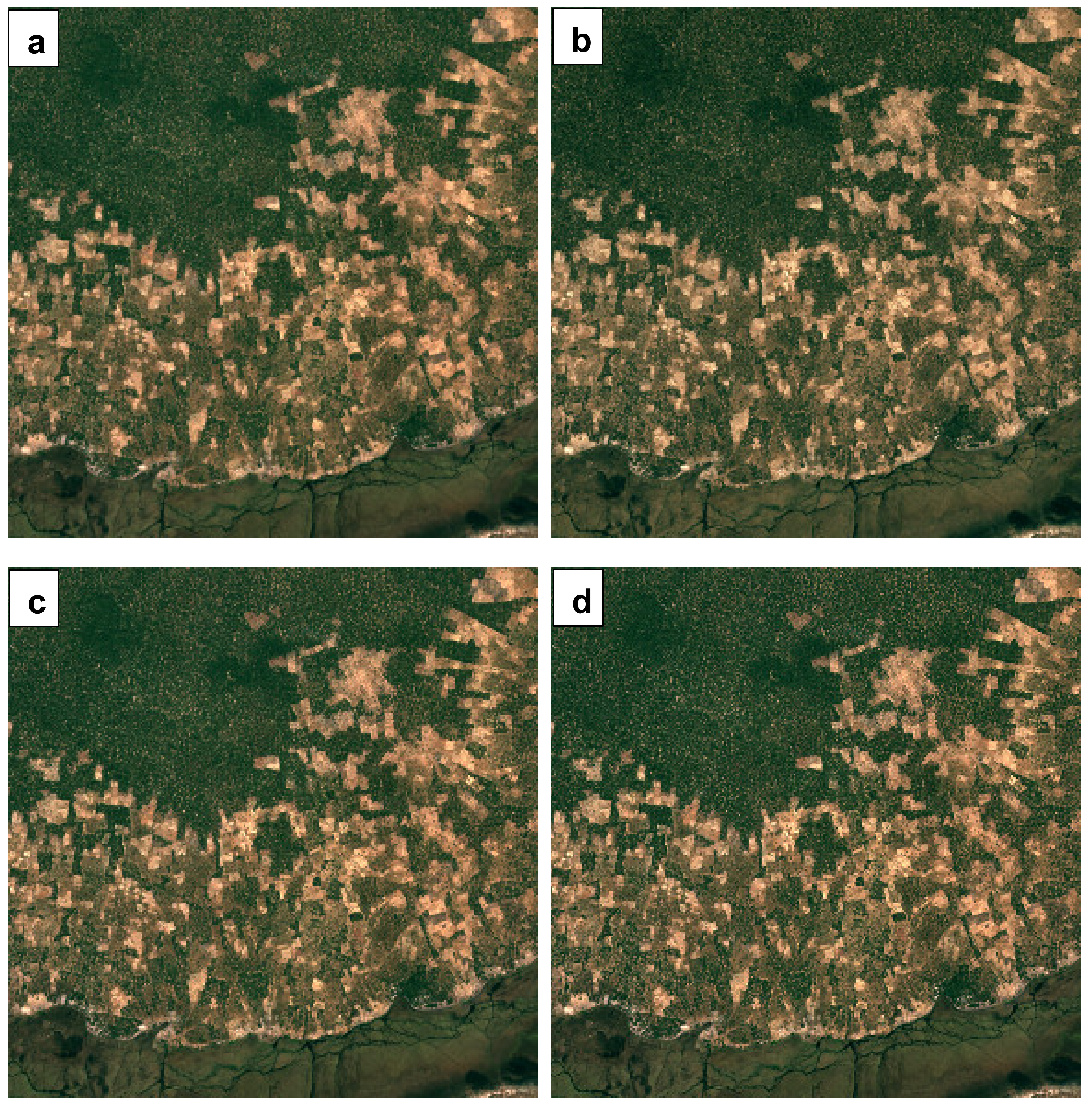
Figure 2.
Study site 2 true color surface reflectance images, composed of 1800 × 1800 3.333 m pixels covering 6 × 6 km (a) Sentinel-2 reflectance bilinear resampled from 10 m, (b) Planetscope reflectance, (c) Sentinel-2 HPM sharpened from 10 m, and (d) Sentinel-2 M3 sharpened from 10 m. Images oriented with north at the top of the image. Site and image dates summarized in Table 2.

Figure 3.
Study site 3 true color surface reflectance images, composed of 1800 × 1800 3.333 m pixels covering 6 × 6 km (a) Sentinel-2 reflectance bilinear resampled from 10 m, (b) Planetscope reflectance, (c) Sentinel-2 HPM sharpened from 10 m, and (d) Sentinel-2 M3 sharpened from 10 m. Images oriented with north at the top of the image. Site and image dates summarized in Table 2.

Figure 4.
Study site 1 false color surface reflectance images, composed of 1800 × 1800 3.333 m pixels covering 6 × 6 km (a) Sentinel-2 NIR (855–875 nm), red-edge (773–793 nm), and SWIR (1565–1655 nm) reflectance bilinear resampled from 20 m, (b) Planetscope NIR reflectance and synthetic Sentinel-2 red-edge and SWIR reflectance, (c) Sentinel-2 false color reflectance HPM sharpened from 20 m, and (d) Sentinel-2 false color reflectance M3 sharpened from 20 m. Images oriented with north at the top of the image. Site and image dates summarized in Table 2.

Figure 5.
Study site 2 false color surface reflectance images, composed of 1800 × 1800 3.333 m pixels covering 6 × 6 km (a) Sentinel-2 NIR (855–875 nm), red-edge (773–793 nm), and SWIR (1565–1655 nm) reflectance bilinear resampled from 20 m, (b) Planetscope NIR reflectance and synthetic Sentinel-2 red-edge and SWIR reflectance, (c) Sentinel-2 false color reflectance HPM sharpened from 20 m, and (d) Sentinel-2 false color reflectance M3 sharpened from 20 m. Images oriented with north at the top of the image. Site and image dates summarized in Table 2.
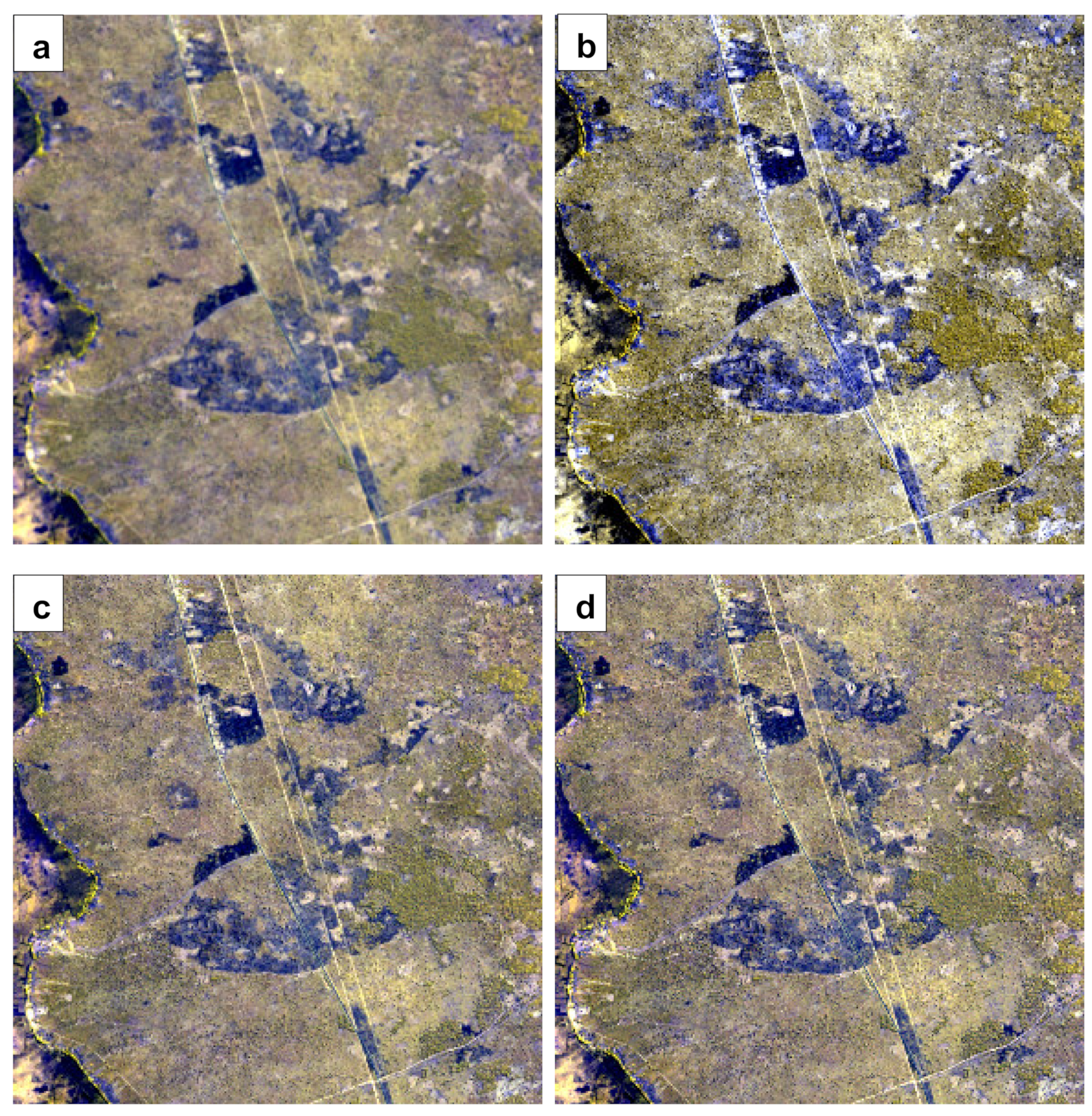
Figure 6.
Study site 3 false color surface reflectance images, composed of 1800 × 1800 3.333 m pixels covering 6 × 6 km (a) Sentinel-2 NIR (855–875 nm), red-edge (773–793 nm), and SWIR (1565–1655 nm) reflectance bilinear resampled from 20 m, (b) Planetscope NIR reflectance and synthetic Sentinel-2 red-edge and SWIR reflectance, (c) Sentinel-2 false color reflectance HPM sharpened from 20 m, and (d) Sentinel-2 false color reflectance M3 sharpened from 20 m. Images oriented with north at the top of the image. Site and image dates summarized in Table 2.
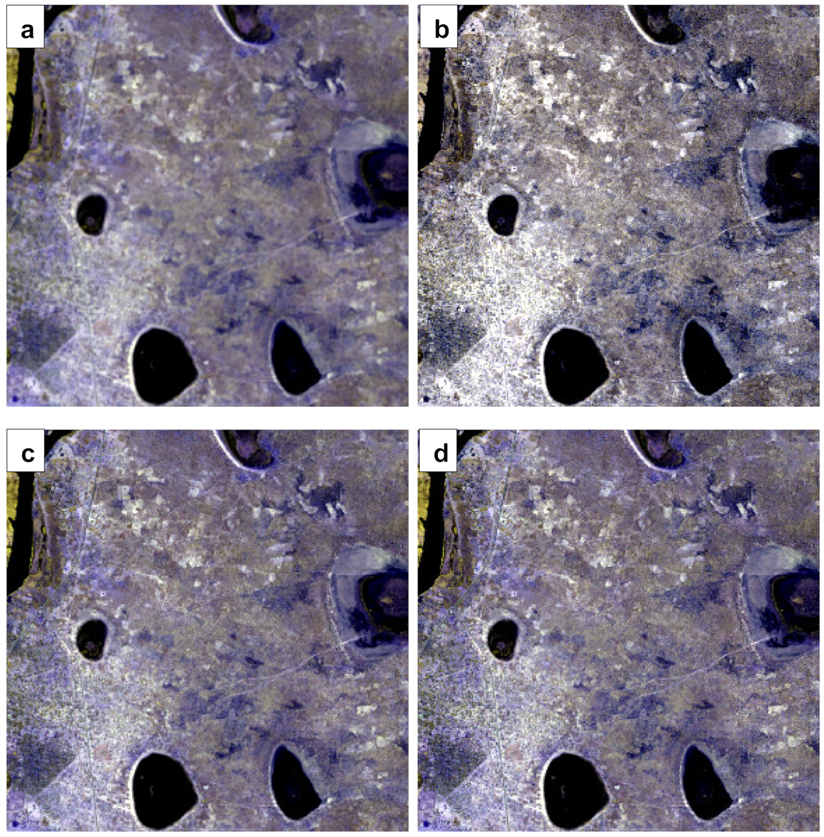
Figure 7.
Study site 1 spatial subset (240 × 240 3.333 m pixels, 0.8 × 0.8 km), top row: true color (red, green, and blue) surface reflectance, third row: false color (NIR 855–875 nm, red-edge 773–793 nm, and SWIR 1565–1655 nm) surface reflectance. The columns show from left to right: Sentinel-2 surface reflectance bilinear resampled to 3.333 m, Planetscope-0 3.333 m surface reflectance, HPM sharpened 3.333 m surface reflectance, and M3 sharpened 3.333 m surface reflectance. The second and fourth rows (greyscale figures) show the root mean square difference (RMSD = ) derived between the Sentinel-2 bilinear resampled reflectance (, left column) and the Planetscope-0 3.333 m, HPM, and M3 sharpened reflectance (, shown in the three right columns). RMSD values are scaled in reflectance units (0–1) multiplied by 10,000.
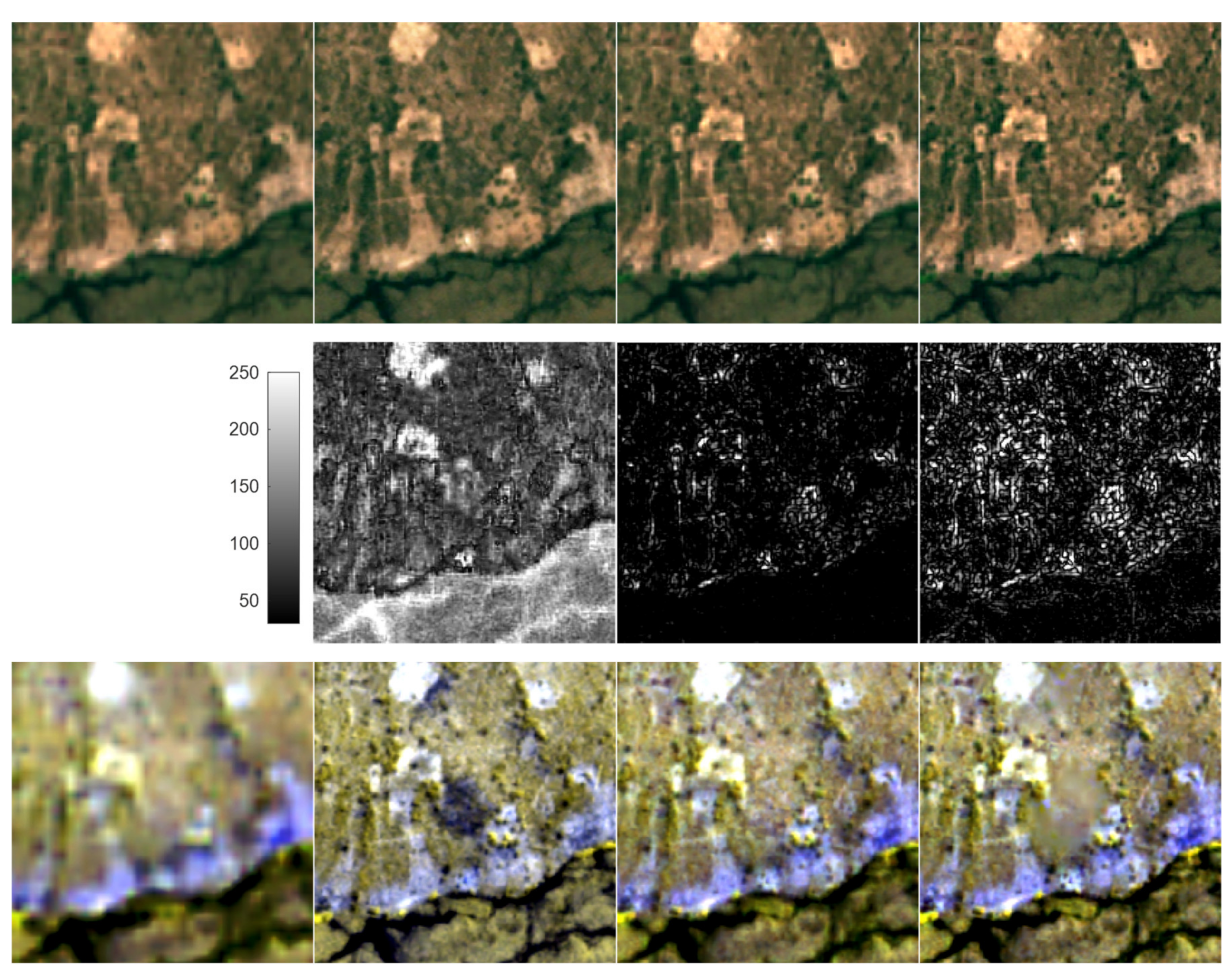

Figure 8.
Study site 2 spatial subset (240 × 240 3.333 m pixels, 0.8 × 0.8 km), top row: true color (red, green, and blue) surface reflectance, third row: false color (NIR 855–875 nm, red-edge 773–793 nm, and SWIR 1565–1655 nm) surface reflectance. The columns show from left to right: Sentinel-2 surface reflectance bilinear resampled to 3.333 m, Planetscope-0 3.333 m surface reflectance, HPM sharpened 3.333 m surface reflectance, and M3 sharpened 3.333 m surface reflectance. The second and fourth rows (greyscale figures) show the root mean square difference (RMSD = ) derived between the Sentinel-2 bilinear resampled reflectance (, left column) and the Planetscope-0 3.333 m, HPM, and M3 sharpened reflectance (, shown in the three right columns). RMSD values are scaled in reflectance units (0–1) multiplied by 10,000.

Figure 9.
Study site 3 spatial subset (240 × 240 3.333 m pixels, 0.8 × 0.8 km), top row: true color (red, green, and blue) surface reflectance, third row: false color (NIR 855–875 nm, red-edge 773–793 nm, and SWIR 1565–1655 nm) surface reflectance. The columns show from left to right: Sentinel-2 surface reflectance bilinear resampled to 3.333 m, Planetscope-0 3.333 m surface reflectance, HPM sharpened 3.333 m surface reflectance, and M3 sharpened 3.333 m surface reflectance. The second and fourth rows (greyscale figures) show the root mean square difference (RMSD = ) derived between the Sentinel-2 bilinear resampled reflectance (, left column) and the Planetscope-0 3.333 m, HPM, and M3 sharpened reflectance (, shown in the three right columns). RMSD values are scaled in reflectance units (0–1) multiplied by 10,000.

| Band | Sentinel-2 | Planetscope-0 | ||
|---|---|---|---|---|
| Band (Bandwidth) | Pixel Size | Band (Bandwidth) | Pixel Size | |
| Blue | 458–523 (65 nm) | 10 m | 455–515 (60 nm) | 3 m |
| Green | 543–578 (35 nm) | 10 m | 500–590 (90 nm) | 3 m |
| Red | 650–680 (30 nm) | 10 m | 590–670 (80 nm) | 3 m |
| Red-edge | 697–713 (16 nm) | 20 m | - | |
| Red-edge | 732–748 (16 nm) | 20 m | - | |
| Red-edge | 773–793 (20 nm) | 20 m | - | |
| NIR | 785–900 (115 nm) | 10 m | 780–860 (80 nm) | 3 m |
| NIR | 855–875 (20 nm) | 20 m | - | |
| SWIR | 1565–1655 (90 nm) | 20 m | - | |
| SWIR | 2100–2280 (180 nm) | 20 m | - | |
Table 2.
Study sites and Sentinel-2B and Planetscope-0 acquisitions.
| Lon/Lat of Top Left Corner | Acquisition Date in 2018 | Acquisition Time (UTC) | |
|---|---|---|---|
| Study site 1 | 23°41′55″ E, 15°40′51″ S | S2B: 30 July Planet: 31 July | S2B: 08:15:59 Planet: 08:08:57 |
| Study site 2 | 23°12′59″ E, 15°27′20″ S | S2B: 30 July Planet: 31 July | S2B: 08:15:59 Planet: 08:12:08 |
| Study site 3 | 23°18′08″ E, 16°03′33″ S | S2B: 30 July Planet: 31 July | S2B: 08:15:59 Planet: 09:05:25 |
Table 3.
Study site values derived considering the four Sentinel-2 10 m sharpened bands (Table 1) together (n = 4). The highest value (least distortion) for each study site is shown in red bold font, and if values are within two decimal places (i.e., |HPM-M3| < 0.01), then both are shown in red bold.
| Bilinear | HPM | M3 | HPM-M3 | |
|---|---|---|---|---|
| Study site 1 | 0.5736 | 0.9328 | 0.9650 | −0.0322 |
| Study site 2 | 0.5777 | 0.9628 | 0.9544 | 0.0084 |
| Study site 3 | 0.6319 | 0.9632 | 0.9599 | 0.0033 |
Table 4.
Study site
values derived considering the four Sentinel-2 10 m sharpened bands independently (n = 1). The highest value (least distortion) for each study site is shown in red bold font, and if values are within two decimal places (i.e., |HPM-M3| < 0.01), then both are shown in red bold.
Table 4.
Study site
values derived considering the four Sentinel-2 10 m sharpened bands independently (n = 1). The highest value (least distortion) for each study site is shown in red bold font, and if values are within two decimal places (i.e., |HPM-M3| < 0.01), then both are shown in red bold.
| 10 m Band | Site | Bilinear | HPM | M3 | HPM-M3 |
|---|---|---|---|---|---|
| Blue | Study site 1 | 0.5845 | 0.9112 | 0.9448 | −0.0336 |
| Study site 2 | 0.5807 | 0.9522 | 0.9309 | 0.0213 | |
| Study site 3 | 0.6231 | 0.9501 | 0.9426 | 0.0075 | |
| Green | Study site 1 | 0.5783 | 0.9355 | 0.9764 | −0.0409 |
| Study site 2 | 0.5769 | 0.9705 | 0.9673 | 0.0032 | |
| Study site 3 | 0.6264 | 0.9672 | 0.9653 | 0.0019 | |
| Red | Study site 1 | 0.5915 | 0.9207 | 0.9730 | −0.0523 |
| Study site 2 | 0.5828 | 0.9653 | 0.9655 | −0.0002 | |
| Study site 3 | 0.6241 | 0.9675 | 0.9615 | 0.0060 | |
| NIR (785–900 nm) | Study site 1 | 0.5080 | 0.9517 | 0.9601 | −0.0084 |
| Study site 2 | 0.5307 | 0.9578 | 0.9504 | 0.0074 | |
| Study site 3 | 0.6257 | 0.9616 | 0.9685 | −0.0069 |
Table 5.
Study site values derived considering the six Sentinel-2 20 m sharpened bands (Table 1) together (n = 6). The highest value (least distortion) for each study site is shown in red bold font, and if values are within two decimal places (i.e., |HPM-M3| < 0.01), then both are shown in red bold.
| Bilinear | HPM | M3 | HPM-M3 | |
|---|---|---|---|---|
| Study site 1 | 0.2856 | 0.9182 | 0.9112 | 0.0070 |
| Study site 2 | 0.2889 | 0.8748 | 0.8625 | 0.0123 |
| Study site 3 | 0.3306 | 0.9020 | 0.9123 | −0.0103 |
Table 6.
Study site values derived considering the six Sentinel-2 20 m sharpened bands independently (n = 1). The highest value (least distortion) for each study site is shown in red bold font, and if values are within two decimal places (i.e., |HPM-M3| < 0.01), then both are shown in red bold.
Table 6.
Study site values derived considering the six Sentinel-2 20 m sharpened bands independently (n = 1). The highest value (least distortion) for each study site is shown in red bold font, and if values are within two decimal places (i.e., |HPM-M3| < 0.01), then both are shown in red bold.
| 20 m Band | Site | Bilinear | HPM | M3 | HPM-M3 |
|---|---|---|---|---|---|
| Red-edge (697–713 nm) | Study site 1 | 0.2702 | 0.9468 | 0.9441 | 0.0027 |
| Study site 2 | 0.2546 | 0.9279 | 0.9221 | 0.0058 | |
| Study site 3 | 0.2959 | 0.9412 | 0.9464 | −0.0052 | |
| Red-edge (732–748 nm) | Study site 1 | 0.2457 | 0.9200 | 0.9176 | 0.0024 |
| Study site 2 | 0.2408 | 0.8869 | 0.8727 | 0.0142 | |
| Study site 3 | 0.2989 | 0.9204 | 0.9228 | −0.0024 | |
| Red-edge (773–793 nm) | Study site 1 | 0.2441 | 0.9115 | 0.9054 | 0.0061 |
| Study site 2 | 0.2433 | 0.8674 | 0.8548 | 0.0126 | |
| Study site 3 | 0.3039 | 0.9179 | 0.9206 | −0.0027 | |
| NIR (855–875 nm) | Study site 1 | 0.2405 | 0.9170 | 0.9038 | 0.0132 |
| Study site 2 | 0.2442 | 0.9175 | 0.8931 | 0.0244 | |
| Study site 3 | 0.3043 | 0.9330 | 0.9458 | −0.0128 | |
| SWIR (1565–1655 nm) | Study site 1 | 0.2536 | 0.8643 | 0.8575 | 0.0068 |
| Study site 2 | 0.2361 | 0.7802 | 0.7657 | 0.0145 | |
| Study site 3 | 0.2715 | 0.8123 | 0.8385 | −0.0262 | |
| SWIR (2100–2280 nm) | Study site 1 | 0.2615 | 0.8636 | 0.8756 | −0.0120 |
| Study site 2 | 0.2712 | 0.8265 | 0.8099 | 0.0166 | |
| Study site 3 | 0.2809 | 0.8057 | 0.8237 | −0.0180 |
Table 7.
Spatial subset values derived considering the four Sentinel-2 10 m sharpened bands (Table 1) together (n = 4). The highest value (least distortion) for each study site is shown in red bold font, and if values are within two decimal places (i.e., |HPM-M3| < 0.01), then both are shown in red bold.
| Bilinear | HPM | M3 | HPM-M3 | |
|---|---|---|---|---|
| Study site 1 | 0.6148 | 0.9438 | 0.9707 | −0.0269 |
| Study site 2 | 0.5512 | 0.9528 | 0.9492 | 0.0036 |
| Study site 3 | 0.6340 | 0.9595 | 0.9589 | 0.0006 |
Table 8.
Spatial subset values derived considering the four Sentinel-2 10 m sharpened bands independently (n = 1). The highest value (least distortion) for each study site is shown in red bold font, and if values are within two decimal places (i.e., |HPM-M3| < 0.01), then both are shown in red bold.
| 10 m band | Site | Bilinear | HPM | M3 | HPM-M3 |
|---|---|---|---|---|---|
| Blue | Study site 1 | 0.6270 | 0.9339 | 0.9606 | −0.0267 |
| Study site 2 | 0.5513 | 0.9574 | 0.9415 | 0.0159 | |
| Study site 3 | 0.6270 | 0.9629 | 0.9571 | 0.0058 | |
| Green | Study site 1 | 0.6230 | 0.9487 | 0.9851 | −0.0364 |
| Study site 2 | 0.5529 | 0.9716 | 0.9688 | 0.0028 | |
| Study site 3 | 0.6248 | 0.9751 | 0.9714 | 0.0037 | |
| Red | Study site 1 | 0.6191 | 0.9499 | 0.9808 | −0.0309 |
| Study site 2 | 0.5589 | 0.9651 | 0.9659 | −0.0008 | |
| Study site 3 | 0.6195 | 0.9712 | 0.9621 | 0.0091 | |
| NIR (785–900 nm) | Study site 1 | 0.5512 | 0.9377 | 0.9354 | 0.0023 |
| Study site 2 | 0.5092 | 0.9261 | 0.8719 | 0.0542 | |
| Study site 3 | 0.6217 | 0.9257 | 0.9141 | 0.0116 |
Table 9.
Spatial subset values derived considering the six Sentinel-2 20 m sharpened bands (Table 1) together (n = 6). The highest value (least distortion) for each study site is shown in red bold font, and if values are within two decimal places (i.e., |HPM-M3| < 0.01), then both are shown in red bold.
| Bilinear | HPM | M3 | HPM-M3 | |
|---|---|---|---|---|
| Study site 1 | 0.2714 | 0.9189 | 0.8770 | 0.0419 |
| Study site 2 | 0.2131 | 0.8036 | 0.8217 | −0.0181 |
| Study site 3 | 0.4330 | 0.8490 | 0.8601 | −0.0111 |
Table 10.
Spatial subsets values derived considering the six Sentinel-2 20 m sharpened bands independently (n = 1). The highest value (least distortion) for each study site is shown in red bold font, and if values are within two decimal places (i.e., |HPM-M3| < 0.01), then both are shown in red bold.
| 20 m band | Site | Bilinear | HPM | M3 | HPM-M3 |
|---|---|---|---|---|---|
| Red-edge (697–713 nm) | Study site 1 | 0.2171 | 0.9592 | 0.9315 | 0.0277 |
| Study site 2 | 0.1792 | 0.8746 | 0.8579 | 0.0167 | |
| Study site 3 | 0.3396 | 0.9213 | 0.9146 | 0.0067 | |
| Red-edge (732–748 nm) | Study site 1 | 0.2386 | 0.8915 | 0.8582 | 0.0333 |
| Study site 2 | 0.1578 | 0.7961 | 0.7216 | 0.0745 | |
| Study site 3 | 0.3454 | 0.8630 | 0.8504 | 0.0126 | |
| Red-edge (773–793 nm) | Study site 1 | 0.2481 | 0.8602 | 0.8325 | 0.0277 |
| Study site 2 | 0.1796 | 0.7644 | 0.6893 | 0.0751 | |
| Study site 3 | 0.3803 | 0.8379 | 0.8292 | 0.0087 | |
| NIR (855–875 nm) | Study site 1 | 0.2569 | 0.8620 | 0.8189 | 0.0431 |
| Study site 2 | 0.1883 | 0.8401 | 0.7469 | 0.0932 | |
| Study site 3 | 0.4097 | 0.8414 | 0.8273 | 0.0141 | |
| SWIR (1565–1655 nm) | Study site 1 | 0.2114 | 0.8740 | 0.7865 | 0.0875 |
| Study site 2 | 0.1516 | 0.7228 | 0.7467 | −0.0239 | |
| Study site 3 | 0.3810 | 0.7030 | 0.7546 | −0.0516 | |
| SWIR (2100–2280 nm) | Study site 1 | 0.2303 | 0.9119 | 0.8877 | 0.0242 |
| Study site 2 | 0.2069 | 0.8022 | 0.7687 | 0.0335 | |
| Study site 3 | 0.3261 | 0.7844 | 0.8322 | −0.0478 |
© 2020 by the authors. Licensee MDPI, Basel, Switzerland. This article is an open access article distributed under the terms and conditions of the Creative Commons Attribution (CC BY) license (http://creativecommons.org/licenses/by/4.0/).
Share and Cite
MDPI and ACS Style
Li, Z.; Zhang, H.K.; Roy, D.P.; Yan, L.; Huang, H. Sharpening the Sentinel-2 10 and 20 m Bands to Planetscope-0 3 m Resolution. Remote Sens. 2020, 12, 2406. https://doi.org/10.3390/rs12152406
AMA Style
Li Z, Zhang HK, Roy DP, Yan L, Huang H. Sharpening the Sentinel-2 10 and 20 m Bands to Planetscope-0 3 m Resolution. Remote Sensing. 2020; 12(15):2406. https://doi.org/10.3390/rs12152406
Chicago/Turabian StyleLi, Zhongbin, Hankui K. Zhang, David P. Roy, Lin Yan, and Haiyan Huang. 2020. "Sharpening the Sentinel-2 10 and 20 m Bands to Planetscope-0 3 m Resolution" Remote Sensing 12, no. 15: 2406. https://doi.org/10.3390/rs12152406
Note that from the first issue of 2016, this journal uses article numbers instead of page numbers. See further details here.