Changes and Predictions of Vertical Distributions of Global Light-Absorbing Aerosols Based on CALIPSO Observation

 ,
,
Abstract
:
1. Introduction
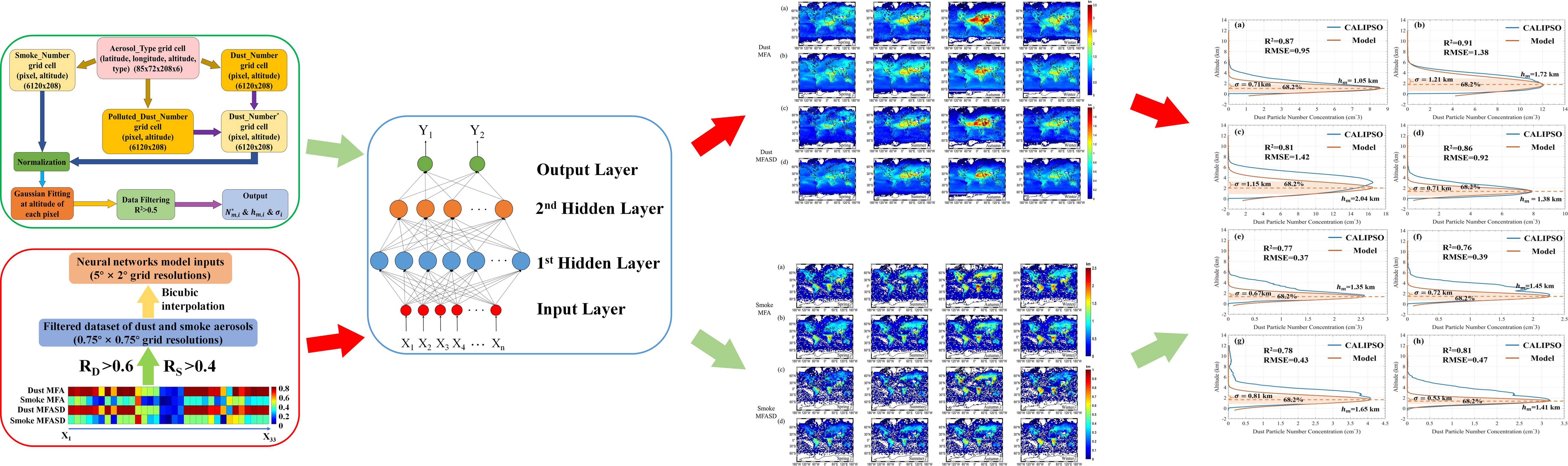
2. Data and Methods
2.1. Data Preparation
2.2. Retrieval of Vertical Distribution Parameters
2.3. Development of the Prediction Model
3. Results
3.1. Seasonal Variations in Dust Aerosols
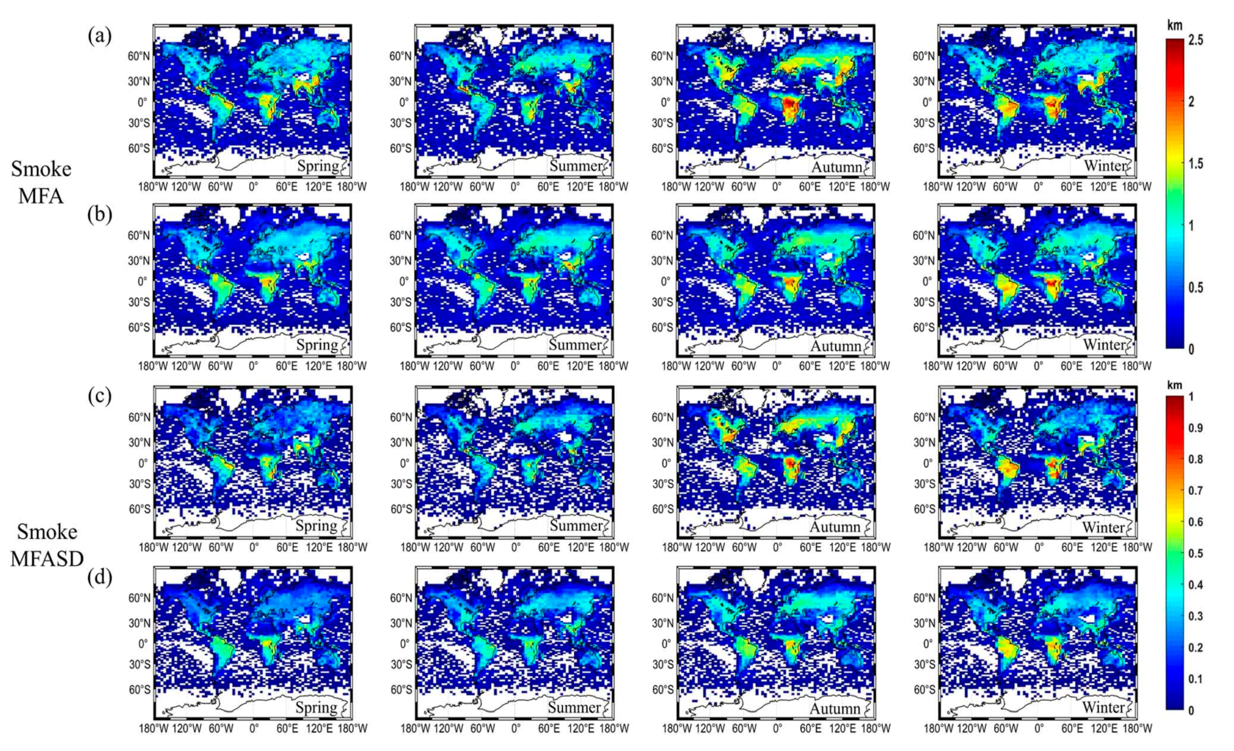
3.2. Seasonal Variations in Smoke Aerosols
3.3. Long-term Changes in Global Dust and Smoke Aerosols
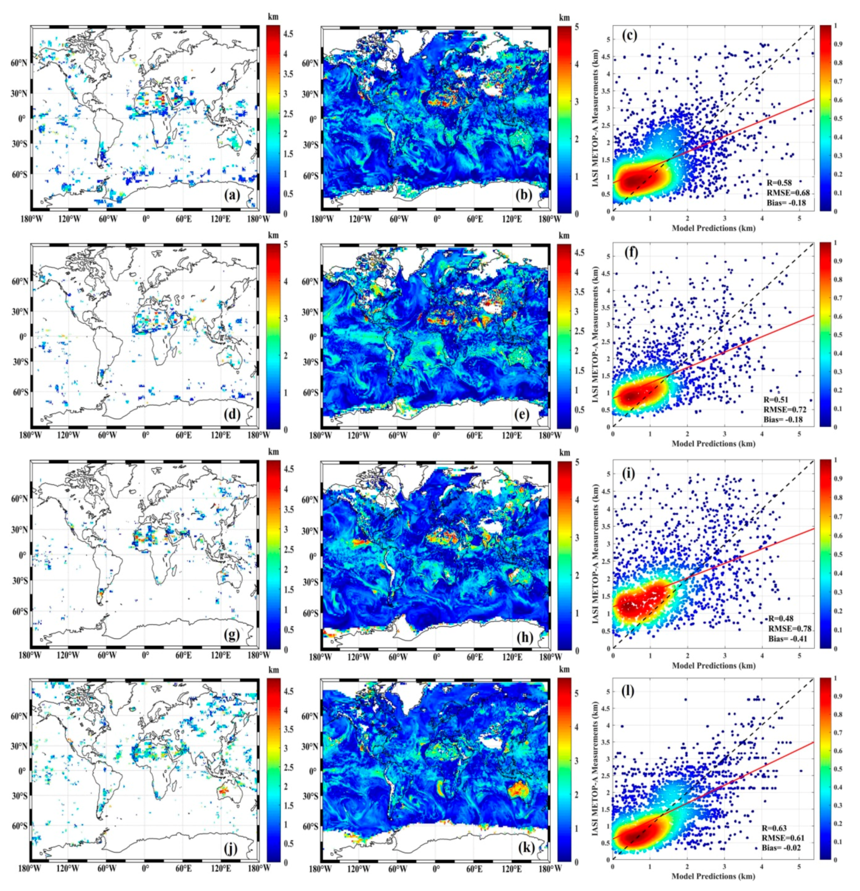
3.4. Prediction of Vertical Distributions of Absorbing Aerosols
4. Discussion
4.1. Spatial-temporal Variations of Absorbing Aerosols
4.2. Predictions of Vertical Distributions of Absorbing Aerosols
5. Conclusions
Author Contributions
Funding
Acknowledgments
Conflicts of Interest
References
- Gordon, H.R.; Du, T.; Zhang, T. Remote sensing of ocean color and aerosol properties: Resolving the issue of aerosol absorption. Appl. Opt. 1997, 36, 8670–8684. [Google Scholar] [CrossRef] [PubMed]
- Myhre, G.; Bellouin, N.; Berglen, T.F.; Berntsen, T.K.; Boucher, O.; Grini, A.; Ivar, S.A.M.; Johnsrud, I.; Micheal, I.M.; Stordal, F.; et al. Comparison of the radiative properties and direct radiative effect of aerosols from a global aerosol model and remote sensing data over ocean. Tellus B Chem. Phys. Meteorol. 2007, 59, 115–129. [Google Scholar] [CrossRef]
- Duforêt, L.; Frouin, R.; Dubuisson, P. Importance and estimation of aerosol vertical structure in satellite ocean-color remote sensing. Appl. Opt. 2007, 46, 1107–1119. [Google Scholar] [CrossRef] [PubMed] [Green Version]
- Taubman, B.F.; Marufu, L.T.; Vant-Hull, B.L.; Piety, C.A.; Doddridge, B.G.; Dickerson, R.R.; Li, Z. Smoke over haze: Aircraft observations of chemical and optical properties and the effects on heating rates and stability. J. Geophys. Res. Space Phys. 2004, 109, D02206-n/a. [Google Scholar] [CrossRef]
- Mahowald, N.M. Aerosol Indirect Effect on Biogeochemical Cycles and Climate. Science 2011, 334, 794–796. [Google Scholar] [CrossRef]
- Wang, M.; Jiang, L. Atmospheric Correction Using the Information From the Short Blue Band. IEEE Trans. Geosci. Remote Sens. 2018, 56, 6224–6237. [Google Scholar] [CrossRef]
- Gordon, H.R. Atmospheric correction of ocean color imagery in the Earth Observing System era. J. Geophys. Res. Space Phys. 1997, 102, 17081–17106. [Google Scholar] [CrossRef]
- Zhang, M.; Hu, C.; Barnes, B.B. Performance of POLYMER Atmospheric Correction of Ocean Color Imagery in the Presence of Absorbing Aerosols. IEEE Trans. Geosci. Remote Sens. 2019, 57, 6666–6674. [Google Scholar] [CrossRef]
- Bond, T.C.; Doherty, S.J.; Fahey, D.W.; Forster, P.M.D.F.; Berntsen, T.; DeAngelo, B.J.; Flanner, M.G.; Ghan, S.; Kärcher, B.; Koch, D.; et al. Bounding the role of black carbon in the climate system: A scientific assessment. J. Geophys. Res. Atmos. 2013, 118, 5380–5552. [Google Scholar] [CrossRef]
- Charlson, R.J.; Schwartz, S.E.; Hales, J.M.; Cess, R.D.; Coakley, J.A.; Hansen, J.E.; Hofmann, D.J.; Schwarz-Sommer, Z.; Saedler, H.; Sommer, H.; et al. Climate Forcing by Anthropogenic Aerosols. Science 1992, 255, 423–430. [Google Scholar] [CrossRef]
- Lin, L.; Gettelman, A.; Fu, Q.; Xu, Y. Simulated differences in 21st century aridity due to different scenarios of greenhouse gases and aerosols. Clim. Chang. 2018, 146, 407–422. [Google Scholar] [CrossRef] [Green Version]
- Gao, B.-C.; Montes, M.J.; Davis, C.O.; Goetz, A.F. Atmospheric correction algorithms for hyperspectral remote sensing data of land and ocean. Remote Sens. Environ. 2009, 113, S17–S24. [Google Scholar] [CrossRef]
- Kang, L.; Chen, S.; Huang, J.; Zhao, S.; Ma, X.; Yuan, T.; Zhang, X.; Xie, T. The Spatial and Temporal Distributions of Absorbing Aerosols over East Asia. Remote Sens. 2017, 9, 1050. [Google Scholar] [CrossRef] [Green Version]
- Han, Y.; Wu, Y.-H.; Wang, T.; Zhuang, B.; Li, S.; Zhao, K. Impacts of elevated-aerosol-layer and aerosol type on the correlation of AOD and particulate matter with ground-based and satellite measurements in Nanjing, southeast China. Sci. Total Environ. 2015, 532, 195–207. [Google Scholar] [CrossRef]
- Guo, J.P.; Zhang, X.Y.; Wu, Y.R.; Zhaxi, Y.; Che, H.Z.; La, B.; Wang, W.; Li, X.W. Spatio-temporal variation trends of satellite-based aerosol optical depth in China during 1980–2008. Atmos. Environ. 2011, 45, 6802–6811. [Google Scholar] [CrossRef]
- Ma, X.; Bartlett, K.; Harmon, K.; Yu, F. Comparison of AOD between CALIPSO and MODIS: Significant differences over major dust and biomass burning regions. Atmos. Meas. Tech. 2013, 6, 2391–2401. [Google Scholar] [CrossRef] [Green Version]
- Young, S.A.; Vaughan, M.; Kuehn, R.E.; Winker, D.M. The Retrieval of Profiles of Particulate Extinction from Cloud–Aerosol Lidar and Infrared Pathfinder Satellite Observations (CALIPSO) Data: Uncertainty and Error Sensitivity Analyses. J. Atmos. Ocean. Technol. 2013, 30, 395–428. [Google Scholar] [CrossRef]
- Cavalieri, O.; Cairo, F.; Fierli, F.; Di Donfrancesco, G.; Snels, M.; Viterbini, M.; Cardillo, F.; Chatenet, B.; Formenti, P.; Marticorena, B.; et al. Variability of aerosol vertical distribution in the Sahel. Atmos. Chem. Phys. Discuss. 2010, 10, 12005–12023. [Google Scholar] [CrossRef] [Green Version]
- Huang, J.; Guo, J.; Wang, F.; Liu, Z.; Jeong, M.-J.; Yu, H.; Zhang, Z.-B. CALIPSO inferred most probable heights of global dust and smoke layers. J. Geophys. Res. Atmos. 2015, 120, 5085–5100. [Google Scholar] [CrossRef]
- Jacobson, M.Z. Strong radiative heating due to the mixing state of black carbon in atmospheric aerosols. Nature 2001, 409, 695–697. [Google Scholar] [CrossRef]
- Yao, J.; Raffuse, S.M.; Brauer, M.; Williamson, G.J.; Bowman, D.M.; Johnston, F.H.; Henderson, S.B. Predicting the minimum height of forest fire smoke within the atmosphere using machine learning and data from the CALIPSO satellite. Remote Sens. Environ. 2018, 206, 98–106. [Google Scholar] [CrossRef]
- Mao, X.; Shen, T.; Feng, X. Prediction of hourly ground-level PM 2.5 concentrations 3 days in advance using neural networks with satellite data in eastern China. Atmos. Pollut. Res. 2017, 8, 1005–1015. [Google Scholar] [CrossRef]
- Nabavi, S.O.; Haimberger, L.; Abbasi, R.; Samimi, C. Prediction of aerosol optical depth in West Asia using deterministic models and machine learning algorithms. Aeolian Res. 2018, 35, 69–84. [Google Scholar] [CrossRef]
- Kow, P.-Y.; Wang, Y.-S.; Zhou, Y.; Kao, I.-F.; Issermann, M.; Chang, L.-C.; Chang, F.-J. Seamless integration of convolutional and back-propagation neural networks for regional multi-step-ahead PM2.5 forecasting. J. Clean. Prod. 2020, 261, 121285. [Google Scholar] [CrossRef]
- Park, Y.; Kwon, B.; Heo, J.; Hu, X.; Liu, Y.; Moon, T. Estimating PM2.5 concentration of the conterminous United States via interpretable convolutional neural networks. Environ. Pollut. 2020, 256, 113395. [Google Scholar] [CrossRef] [PubMed]
- Xiao, F.; Wong, M.S.; Lee, K.-H.; Campbell, J.R.; Shea, Y.-K. Retrieval of dust storm aerosols using an integrated Neural Network model. Comput. Geosci. 2015, 85, 104–114. [Google Scholar] [CrossRef]
- Huang, L.; Jiang, J.H.; Tackett, J.L.; Su, H.; Fu, R. Seasonal and diurnal variations of aerosol extinction profile and type distribution from CALIPSO 5-year observations. J. Geophys. Res. Atmos. 2013, 118, 4572–4596. [Google Scholar] [CrossRef]
- Hsu, N.C.; Gautam, R.; Sayer, A.M.; Bettenhausen, C.; Li, C.; Jeong, M.J.; Tsay, S.-C.; Holben, B.N. Global and regional trends of aerosol optical depth over land and ocean using SeaWiFS measurements from 1997 to 2010. Atmos. Chem. Phys. Discuss. 2012, 12, 8037–8053. [Google Scholar] [CrossRef] [Green Version]
- Gonzalez-Alonso, L.; Martin, M.V.; Kahn, R.A. Biomass-burning smoke heights over the Amazon observed from space. Atmos. Chem. Phys. Discuss. 2019, 19, 1685–1702. [Google Scholar] [CrossRef] [Green Version]
- Winker, D.M.; Vaughan, M.; Omar, A.; Hu, Y.; Powell, K.A.; Liu, Z.; Hunt, W.H.; Young, S.A. Overview of the CALIPSO Mission and CALIOP Data Processing Algorithms. J. Atmos. Ocean. Technol. 2009, 26, 2310–2323. [Google Scholar] [CrossRef]
- Pan, H.; Wang, M.; Kumar, K.R.; Lu, H.; Mamtimin, A.; Huo, W.; Yang, X.; Yang, F.; Zhou, C. Seasonal and vertical distributions of aerosol type extinction coefficients with an emphasis on the impact of dust aerosol on the microphysical properties of cirrus over the Taklimakan Desert in Northwest China. Atmos. Environ. 2019, 203, 216–227. [Google Scholar] [CrossRef]
- Rémy, S.; Veira, A.; Paugam, R.; Sofiev, M.; Kaiser, J.W.; Marenco, F.; Burton, S.P.; Benedetti, A.; Engelen, R.; Ferrare, R.; et al. Two global data sets of daily fire emission injection heights since 2003. Atmos. Chem. Phys. Discuss. 2017, 17, 2921–2942. [Google Scholar] [CrossRef] [Green Version]
- Klüser, L.; Banks, J.R.; Martynenko, D.; Bergemann, C.; Brindley, H.; Holzer-Popp, T. Information content of space-borne hyperspectral infrared observations with respect to mineral dust properties. Remote Sens. Environ. 2015, 156, 294–309. [Google Scholar] [CrossRef] [Green Version]
- Barnes, J.E.; Sharma, N.C.P.; Kaplan, T.B. Atmospheric aerosol profiling with a bistatic imaging lidar system. Appl. Opt. 2007, 46, 2922–2929. [Google Scholar] [CrossRef] [PubMed]
- Guo, J.; Xia, F.; Zhang, Y.; Liu, H.; Li, J.; Lou, M.; He, J.; Yan, Y.; Wang, F.; Min, M.; et al. Impact of diurnal variability and meteorological factors on the PM2.5—AOD relationship: Implications for PM2.5 remote sensing. Environ. Pollut. 2017, 221, 94–104. [Google Scholar] [CrossRef] [Green Version]
- Li, X.; Cheng, X.; Wu, W.; Wang, Q.; Tong, Z.; Zhang, X.; Deng, D.; Li, Y. Forecasting of bioaerosol concentration by a Back Propagation neural network model. Sci. Total Environ. 2020, 698, 134315. [Google Scholar] [CrossRef]
- Lakshmi, N.B.; Babu, S.S.; Nair, V.S. Recent Regime Shifts in Mineral Dust Trends Over South Asia From Long-Term CALIPSO Observations. IEEE Trans. Geosci. Remote Sens. 2019, 57, 1–5. [Google Scholar] [CrossRef]
- Kazil, J.; Stier, P.; Zhang, K.; Quaas, J.; Kinne, S.; O’Donnell, D.; Rast, S.; Esch, M.; Ferrachat, S.; Lohmann, U.; et al. Aerosol nucleation and its role for clouds and Earth’s radiative forcing in the aerosol-climate model ECHAM5-HAM. Atmos. Chem. Phys. Discuss. 2010, 10, 10733–10752. [Google Scholar] [CrossRef] [Green Version]
- Peers, F.; Waquet, F.; Cornet, C.; Dubuisson, P.; Ducos, F.; Goloub, P.; Szczap, F.; Tanre, D.; Thieuleux, F. Absorption of aerosols above clouds from POLDER/PARASOL measurements and estimation of their direct radiative effect. Atmos. Chem. Phys. Discuss. 2015, 15, 4179–4196. [Google Scholar] [CrossRef] [Green Version]
- Huang, G.-B. Learning capability and storage capacity of two-hidden-layer feedforward networks. IEEE Trans. Neural Netw. 2003, 14, 274–281. [Google Scholar] [CrossRef] [Green Version]
- Dahutia, P.; Pathak, B.; Bhuyan, P.K. Vertical distribution of aerosols and clouds over north-eastern South Asia: Aerosol-cloud interactions. Atmos. Environ. 2019, 215, 116882. [Google Scholar] [CrossRef]
- Proestakis, E.; Amiridis, V.; Marinou, E.; Georgoulias, A.K.; Solomos, S.; Kazadzis, S.; Chimot, J.; Che, H.; Alexandri, G.; Binietoglou, I.; et al. Nine-year spatial and temporal evolution of desert dust aerosols over South and East Asia as revealed by CALIOP. Atmos. Chem. Phys. Discuss. 2018, 18, 1337–1362. [Google Scholar] [CrossRef] [Green Version]
- Sheehan, P.E.; Bowman, F.M. Estimated effects of temperature on secondary organic aerosol concentrations. Environ. Sci. Technol. 2001, 35, 2129–2135. [Google Scholar] [CrossRef]
- Shi, S.; Cheng, T.; Gu, X.; Guo, H.; Wu, Y.; Wang, Y. Biomass burning aerosol characteristics for different vegetation types in different aging periods. Environ. Int. 2019, 126, 504–511. [Google Scholar] [CrossRef] [PubMed]
- Alam, K.; Qureshi, S.; Blaschke, T. Monitoring spatio-temporal aerosol patterns over Pakistan based on MODIS, TOMS and MISR satellite data and a HYSPLIT model. Atmos. Environ. 2011, 45, 4641–4651. [Google Scholar] [CrossRef]
- Nenes, A.; Krom, M.D.; Mihalopoulos, N.; Van Cappellen, P.; Shi, Z.; Bougiatioti, A.; Zarmpas, P.; Herut, B. Atmospheric acidification of mineral aerosols: A source of bioavailable phosphorus for the oceans. Atmos. Chem. Phys. Discuss. 2011, 11, 6265–6272. [Google Scholar] [CrossRef] [Green Version]
- Jickells, T.; An, Z.S.; Andersen, K.K.; Baker, A.R.; Bergametti, G.; Brooks, N.; Cao, J.; Boyd, P.W.; Duce, R.A.; Hunter, K.A.; et al. Global Iron Connections Between Desert Dust, Ocean Biogeochemistry, and Climate. Science 2005, 308, 67–71. [Google Scholar] [CrossRef] [Green Version]
- Kylling, A.; Vandenbussche, S.; Capelle, V.; Cuesta, J.; Klüser, L.; Lelli, L.; Holzer-Popp, T.; Stebel, K.; Veefkind, P. Comparison of dust-layer heights from active and passive satellite sensors. Atmos. Meas. Tech. 2018, 11, 2911–2936. [Google Scholar] [CrossRef] [Green Version]
- Vadrevu, K.P.; Lasko, K.; Giglio, L.; Justice, C. Vegetation fires, absorbing aerosols and smoke plume characteristics in diverse biomass burning regions of Asia. Environ. Res. Lett. 2015, 10, 105003. [Google Scholar] [CrossRef] [Green Version]
- Myhre, G.; Samset, B.; Schulz, M.; Balkanski, Y.; Bauer, S.; Berntsen, T.K.; Bian, H.; Bellouin, N.; Chin, M.; Diehl, T.; et al. Radiative forcing of the direct aerosol effect from AeroCom Phase II simulations. Atmos. Chem. Phys. Discuss. 2013, 13, 1853–1877. [Google Scholar] [CrossRef] [Green Version]


| Input | Description | Input | Description |
|---|---|---|---|
| X1 | Relative humidity at 1000 hPa | X18 | Vertical integral of divergence of geopotential flux |
| X2 | Relative humidity at 950 hPa | X19 | Vertical integral of divergence of kinetic energy flux |
| X3 | Relative humidity at 900 hPa | X20 | Vertical integral of potential and internal energy |
| X4 | Relative humidity at 850 hPa | X21 | Vertical integral of temperature |
| X5 | Relative humidity at 800 hPa | X22 | Vertical integral of thermal energy |
| X6 | Evaporation | X23 | Vertical integral of water vapor |
| X7 | Mean sea level pressure | X24 | Albedo |
| X8 | 10 m wind speed | X25 | Boundary layer height |
| X9 | Skin temperature | X26 | Surface roughness for heat |
| X10 | Surface pressure | X27 | Surface roughness |
| X11 | Soil temperature | X28 | Surface latent heat flux |
| X12 | Volumetric soil water | X29 | Surface sensible heat flux |
| X13 | Total column cloud ice water | X30 | Surface net solar radiation |
| X14 | Total column cloud liquid water | X31 | Surface solar radiation downwards |
| X15 | Total precipitation | X32 | Top net solar radiation |
| X16 | 10 m wind speed of U component | X33 | Top net thermal radiation |
| X17 | 10 m wind speed of V component |
© 2020 by the authors. Licensee MDPI, Basel, Switzerland. This article is an open access article distributed under the terms and conditions of the Creative Commons Attribution (CC BY) license (http://creativecommons.org/licenses/by/4.0/).
Share and Cite
Song, Z.; He, X.; Bai, Y.; Wang, D.; Hao, Z.; Gong, F.; Zhu, Q. Changes and Predictions of Vertical Distributions of Global Light-Absorbing Aerosols Based on CALIPSO Observation. Remote Sens. 2020, 12, 3014. https://doi.org/10.3390/rs12183014
Song Z, He X, Bai Y, Wang D, Hao Z, Gong F, Zhu Q. Changes and Predictions of Vertical Distributions of Global Light-Absorbing Aerosols Based on CALIPSO Observation. Remote Sensing. 2020; 12(18):3014. https://doi.org/10.3390/rs12183014
Chicago/Turabian StyleSong, Zigeng, Xianqiang He, Yan Bai, Difeng Wang, Zengzhou Hao, Fang Gong, and Qiankun Zhu. 2020. "Changes and Predictions of Vertical Distributions of Global Light-Absorbing Aerosols Based on CALIPSO Observation" Remote Sensing 12, no. 18: 3014. https://doi.org/10.3390/rs12183014