Background Tropospheric Delay in Geosynchronous Synthetic Aperture Radar


College of Electronic Science and Technology, National University of Defense Technology (NUDT), Changsha 410073, China
*
Author to whom correspondence should be addressed.
Remote Sens. 2020, 12(18), 3081; https://doi.org/10.3390/rs12183081
Submission received: 26 June 2020
/
Revised: 17 September 2020
/
Accepted: 18 September 2020
/
Published: 20 September 2020
(This article belongs to the Section Atmospheric Remote Sensing)
Abstract
:Spaceborne synthetic aperture radar (SAR) has been treated as a weather independent system for a long time. However, with the development of advanced SAR configurations, e.g., high resolution, bistatic, geosynchronous (GEO), the influence of tropospheric propagation error, which strongly depends on the weather, has begun to receive attention. In this paper, we focus on the effect of deterministic background tropospheric delay (BTD) during the image formation of GEO SAR. First, the decorrelation problems caused by the spatial variation and BTD are presented. Second, by combining with the SAR imaging geometry, the BTD error is decomposed as constant error, spatially variant error, and time variant error, the influences of which are analyzed under different circumstances. Third, an imaging method starting from the meteorological parameters and the GEO SAR systematic parameters is proposed to deal with the decorrelation problems. Finally, simulations with the dot-matrix targets are performed to validate the imaging method.
1. Introduction
With the great advantages in day and night and weather independent observation, spaceborne synthetic aperture radar (SAR) has been widely used in Earth remote sensing since the first civilian SAR satellite “Seasat” was launched by the National Aeronautics and Space Administration (NASA) in 1978. The application scope includes Earth and ocean observation, environmental and climate change research, 3D mapping, and military applications. As the need arises for high resolution, long dwell time observation, the advanced SAR configurations, e.g., high squint, spotlight, staring spotlight, bistatic, and geosynchronous (GEO), are proposed, and several excellent systems are already being operated. GEO SAR is a type of spaceborne SAR system in a geosynchronous orbit with a certain inclination and eccentricity. With the typical footprints of type “–” [1], type “8” [2], and type “O” [3], it has an ultra-long integration time, wide swath, long dwell time, and short revisit time and has great potential in many areas, such as Earthquake prediction, disaster monitoring, and environment observation. Several conceptual systems have been proposed, and more details can be found in [2,4].
As an important error source of spaceborne SAR, propagation error has been paid attention to for a long time. According to the generation mechanism, the propagation error can be subdivided into background tropospheric delay (BTD), turbulent tropospheric delay (TTD), ionospheric dispersion, scintillation, Faraday rotation, and so on [5]. A full discussion of the generation, estimation, and compensation mechanisms of TTD was carried out in [6]. The influence and compensation of the ionospheric effect was considered in [7,8,9]. In this paper, we focus on the BTD in GEO SAR image formation, which relies on the meteorological parameters. The main purpose of this paper is to correct the conventional wisdom of the “weather independent” character of spaceborne SAR and arrive at the fact that the influence of BTD should also be considered in the high requirement SAR configurations, e.g., GEO SAR survey.
Related discussions have appeared in several papers. Prats et al. modeled the tropospheric delay (TD) using an exponential function of the target height [10] in very high resolution spaceborne SAR data processing [11]. Yu et al. introduced a stable tropospheric delay model in high resolution SAR imaging, which was proposed by the European Geostationary Navigation Overlay Service (EGNOS) [12]. Rodon et al. retrieved the stochastic atmospheric phase screen (APS) with a phase gradient algorithm (PGA), where the point scatters distributed in different azimuth positions with good point quality are necessary [1]. Guarnieri et al. proposed an interferometric based autofocus algorithm to retrieve the APS, where an extra reference image acquired in the same subaperture without any atmospheric propagation influence is required [13]. Following the studies above, we put forward a tropospheric delay model to describe the variations in both the space and time domains in GEO SAR survey, which divides the delays into a deterministic background component and a random turbulent one, incorporating recent meteorological data for the characterization of the troposphere, where the modified Saastamoinen model [14,15], Askne model [16], Vienna mapping function [17], Matérn covariance function [18], and random walk process [19] are included [20].
Based on the tropospheric delay model proposed in [20], we introduce the “weather dependent” factor into the spatially variant slant range model to explore the effect of BTD on GEO SAR image formation. Next, the influences of the variations of meteorological parameters on the GEO SAR imaging are decomposed as constant error, spatially variant error, and time variant error and analyzed, respectively. Subsequently, with the input of the systematic and meteorological parameters, an FFT-based imaging method based on the Taylor expansion, series reversion, and nonlinear chirp scaling is proposed to compensate the BTD and spatial variations.
The structure of the paper is as follows. Section 2 presents the decorrelation problems caused by the spatial variation and BTD error in GEO SAR. Section 3 analyzes the influence of BTD on the GEO SAR image formation with the decomposition of constant error, spatially variant error, and time variant error. Section 4 discusses the imaging method of GEO SAR to compensate the spatial variation and BTD error. Section 5 performs the simulation experiments of dot-matrix targets to validate the proposed method. Section 6 summarizes the conclusions of the paper.
2. Decorrelation Problems of Spatial Variation and BTD Error in the GEO SAR Configuration
The slant range history plays an important role in SAR image formation. In order to inquire the influence of spatial variation and BTD error in the GEO SAR configuration, the slant range model is rebuilt as:
where represents the azimuth time (slow time) in the orbit, represents the (along-track and cross-track) positional coordinates of the target in the scene, with being the azimuth time in the scene and being the central slant range of the target, and the subscripts a and r stand for the azimuth and range directions in SAR geometry, respectively. In order to make the variables in the expression clearer, here, we define the data lengths of subscript variables , , as , , , respectively. [] is the set of relevant meteorological parameters, e.g., the surface pressure [], the surface temperature [], and the surface water vapor pressure [], which will be further defined in Expression (6). The illustration of GEO SAR image formation with the influence of BTD error is shown in Figure 1a. It is well known that the decorrelation problem is caused by the phase variation during SAR image formation, i.e., the slant range variation. The first term in Expression (1) is the Euclidean geometric distance between the satellite position [] and the target position [], where 3 means the three-dimensional (3D) coordinates. It contains the spatial variation (azimuth and range in SAR geometry) depending on the satellite trajectory, antenna pattern, and the targets’ position. The second term in Expression (1) represents the BTD error, which depends on the meteorological parameters and incident angle [], which, in turn, depends on the positions of the satellite and target. Subsequently, the decorrelation factors of two terms are considered, and the accurate models are introduced.
2.1. Geometric Distance Model
GEO SAR is characterized by its high orbit, curve trajectory, wide swath, and long integration time, which bring great challenges to the SAR slant range model. Compared with the traditional low Earth orbit (LEO) SAR, the main differences can be summarized as three aspects:
(1) Effect of the curve trajectory: With the long integration time, the satellite trajectory cannot be approximated as a straight line, and the high order slant range model, which can accurately represent the curve trajectory, should be introduced. The direct effect of curve trajectory is that a bulk phase error is introduced in the focused image if the classical range-Doppler or chirp scaling algorithms based on the linear trajectory are used. Related validations have been reported in some papers [21,22,23].
(2) Effect of the curve surface: With the wide swath, the Earth’s surface cannot be approximated as a plane. In the traditional SAR geometric model, an efficient and simple way to model the scene is that the Earth’s surface is treated as a plane with the targets uniformly distributed in the scene. Then, the satellite coordinates and the scene coordinates are connected by a coordinate rotation matrix, which depends on the antenna pattern, position, and velocity of satellite. In this paper, a less efficient, but more accurate modeling method is introduced to reduce the effect of the curve surface. The main idea is that with the position and velocity of the satellite derived from the six orbital elements at different azimuth times, the 3D coordinates of the pixels with different azimuth times and slant ranges in the scene are calculated by combining the equations of the antenna pointing line and the ellipsoid model of the Earth.
(3) Effect of Earth’s rotation: In the traditional SAR configuration, the integration time varies from orders of seconds, and the effect of Earth’s rotation is very weak and can be ignored. However, the integration time increases to several minutes and even several hours in GEO SAR survey. The variation caused by the Earth’s rotation increases accordingly, the influence of which should not be ignored any longer. In the traditional modeling method, a time-varying coordinate rotation matrix should be introduced to build the relationship between the satellite and the scene, which is much less efficient. In this paper, for the different azimuth times, the parameters of the satellite are transferred into the Earth-centered Earth-fixed (ECEF) coordinates. Combining the consideration of Aspect 2, the models of the satellite and scene are unified under the framework of the ECEF coordinates.
With all the considerations above, an accurate geometric distance model is built. First, instead of the linear trajectory, which has been fully applied in the air-borne SAR and low resolution LEO SAR, an accurate elliptical trajectory based on six orbital elements is introduced, and the 3D position and velocity vectors of satellites ( and ) can be achieved. Then, based on the elliptical trajectory, the modeling of the scene is carried out. With the position and velocity of the satellite, the squint angle, and the slant range, the target coordinate on the surface can be calculated by combining with the equation of the elliptical surface of the Earth, i.e.,
where is the central squint angle, is the velocity of the satellite, means the angle between vectors A and B, and and are the semi-major axis and semi-minor axis of the Earth. If we define the scene as a two-dimensional grid varying with and , the 3D coordinates of the targets in the scene with different and can be derived, which is indexed as . Since the coordinates are reached with the equation of the elliptical surface of the Earth, the effect of the curve surface during the wide swath SAR image formation can be reflected in .
In the end, the effect of the Earth’s rotation is considered. The time-varying rotated matrix is introduced into Equation (2), where and can be expressed as:
where represents the angle velocity of Earth’s rotation.
It should be noted that the influences of orbital perturbation caused by the gravity of the Sun and Moon and the effect of terrain relief are ignored for the moment.
With the accurate slant range calculation for different targets with divergent and , a spatially variant high order model with Taylor expansion near can be built, i.e.,
where means the ith-order coefficient and is the error of the ith-order coefficient caused by the spatial variation. A full description of the calculations of the coefficients, order selection, and approximation error control can be found in [23,24].
2.2. BTD Error Model
It is generally accepted that the troposphere can be treated as a nondispersive shell [5]. The propagation delay through the troposphere is caused by two effects: (1) the smaller propagation velocity of the radar waves in the troposphere than in the vacuum; (2) the curvature of the propagation path caused by the dependence of the refractive index with height in side-looking observations. According to the different distribution characteristics, the tropospheric delay can be divided as a deterministic background component (i.e., BTD) and a random turbulent one (i.e., TTD), as shown in Figure 1b [20]. The deterministic background component varies slowly with time and space, which can be estimated with the meteorological parameters. The random turbulent component is stochastically distributed following Kolmogorov’s power law or a power spectrum based on the Matérn-like covariance function. Due to the uncertainty of the turbulent component, the influence of which should be compensated by the autofocus strategy, in this paper, we mainly focus on the influence, error analysis, and compensation of BTD.
According to [25], BTD can be modeled as the superposition of a hydrostatic and wet component, i.e.,
with:
where and are the zenith hydrostatic and wet delays and and are the mapping functions, which allow for the transformation of the zenith into slant delay for the hydrostatic and wet components, respectively. is the lapse rate of the temperature with height, and is the weighted mean temperature.
Zenith hydrostatic delay (ZHD) depends on the air pressure, temperature, local latitude, and height, and the modified Saastamoinen model of ZHD can be expressed as,
where , , , , and h stands for altitude.
Zenith wet delay (ZWD) depends on the temperature, water vapor pressure, local latitude, and height, and the Askne model of ZWD can be expressed as,
where 16.6 K/hPa, 377,600 K2/hPa, and is the water vapor pressure height factor.
Vienna models for and are listed in Equations (9) and (11). The values of the related coefficients are listed in Table 1. The other parameters () can be achieved through the global pressure and temperature 2 wet (GPT2w) model with different local latitude, longitude, and day of year [26,27,28].
with:
where means the incident angle on the line of sight and means the local latitude.
3. Error Analysis of Background Tropospheric Delay
In the framework of SAR geometry, the BTD error is divided into constant error, spatially variant error, and time variant error according to the influence of BTD error on the impulse response of the point target, which are illustrated in Figure 2. The error analyses are performed in this section, which starts from the changing of the meteorological parameters and ends with the influence on the focusing results of point targets.
3.1. Constant Error
The constant error represents the bulk tropospheric delay error during the synthetic aperture of one target. In order to analyze the constant error, the variable isolation method is introduced, i.e., when one variable is analyzed, the others are fixed at a normal value. In this section, the changing of the typical meteorological parameters, i.e., , , and , is analyzed. According to Equations (7) and (8), the variations of ZHD and ZWD are plotted in Figure 3. It is seen that ZHD mainly depends on , and ZWD on , .
Assuming , , and , Equation (7) can be simplified as:
Expanding with around 273.15 K,
Therefore, the partial derivatives of with respect to are approximated as , and the partial derivatives with respect to are approximated as . It can be concluded that is more sensitive to than to . When the pressure changes to 10 hPa, varies by around 2 cm. However, when the temperature changes to only varies by 2 mm.
A similar analysis can be carried out on with the assumption that , , , , i.e.,
The partial derivatives of with respect to are approximated as mm/K, and the partial derivatives with respect to are approximated as mm/hPa. It can be concluded that is more sensitive to than to . When the pressure changes to 10 hPa, varies by around 14 cm. However, when the temperature changes to 10 C, only varies by 7.5 mm.
The changing of constant errors caused by the variation of the meteorological parameters, denoted as and , are compared with the azimuth resolutions of the typical spaceborne SAR systems, as shown in Table 2. The results are shown in Figure 4 and Figure 5, where 1/10 times the azimuth resolutions of TerraSAR (0.15 m), ALOS-PSAR (1 m), GF-3 (1 m), and GEO SAR (2 m) are plotted as references. It is seen that no matter the or , the changes caused by the temperature are very small and can be ignored. Relatively speaking, the changes caused by the pressure are much larger. When the varying of air pressure reaches 30 hPa, is larger than 1/10 times the azimuth resolution of TerraSAR. When the varying of the water vapor pressure reaches 20 hPa, is larger than 1/10 times the azimuth resolution of TerraSAR, GF3, and ALOSPSAR.
From the analysis above, it can be concluded that the constant error of BTD only introduces a bulk phase error, which has no effect on the target focusing and only influences the position of the target. Compared with the resolutions of the typical SAR systems and GEO SAR, the position bias caused by the variation of the meteorological parameters is also very weak and can be ignored.
3.2. Spatially Variant Error
In this paper, the spatially variant error is defined as the error introduced by the mapping function of ZHD and ZWD during the synthetic aperture, where ZHD and ZWD are fixed. In other words, only the delay error caused by the changing of SAR geometry (incident angle) is considered. Within the GEO SAR observation geometry, the incident angle on the line of sight in the mapping functions can be approximated as:
where and represent the elevation incidence and the instantaneous squint angle, respectively. In order to simplify the analysis, we assume that the SAR system works in side-looking mode, i.e., the squint angle at the central time of synthetic aperture equals zero.
The influence on the azimuth impulse response caused by the spatially variant error of BTD is analyzed. A simplified 1D SAR signal model in the azimuth direction is built,
where means the integration time, and represent the central coordinate of the scene, and means the wavelength. The azimuth impulse response can be achieved by an azimuth matched filtering, where the phase error introduced by would cause the defocusing. Since the integration time varies greatly with different carrier frequencies in the GEO SAR configuration, we considered the typical X band (9.65 GHz), C band (5.4 GHz), and L band (1.25 GHz) cases with the related integration times and resolutions. The simulation results near the Equator () with the typical m and m are shown in Figure 6, where the blue dotted line represents the ideal result and the red solid line represents the influenced result. It has been widely accepted that the higher carrier frequency system is more sensitive to the BTD error [29]. While from the figures, it is seen that the influences on azimuth impulse responses with the X band (in Figure 6a) and C band (in Figure 6b) are weak, the influence on the L band ones (in Figure 6c) is relatively serious. In order to give a reasonable explanation, further investigation is carried out. Ignoring the weak difference between the mapping functions of ZHD and ZWD (relying on the height or not) and introducing Equation (16), we express the phase error caused by the spatial error of BTD with a degradation model, i.e.,
where means the spatial error of BTD, which includes both the ZHD and ZWD components, the BTD at the center of the synthetic aperture, and the squint angle at the edge of the synthetic aperture. Considering the linear trajectory model, the phase error can be further derived as:
According to Equation (19), with the fixed azimuth antenna length, the phase error caused by the spatially variant error of BTD is proportional to the wavelength in stripmap mode. This conclusion is consistent with the simulation results.
By comparing the different situations in Figure 6, it is seen that even the integration time reaches 1000 s, and the resolution is 0.72 m, so the influence of the spatial error of BTD is still very weak. Therefore, we can conclude that the spatial error of BTD can be ignored in most cases in the orbit-inclined GEO SAR systems.
3.3. Time Variant Error
After considering the spatial error of BTD, we continue to analyze the influence of the time variant error of BTD. First of all, it should be noted that the time variant error here includes both the varying of BTD with different punctures when the radar position is changing with the azimuth time and the varying of BTD itself during the integration time. According to the previous studies, the gradient of BTD is about 1 cm/km [11]. In this paper, three different variant cases are considered, as shown in Figure 7. Cases 0, 1, and 2 represent the linear, quadratic, and cubic variations, respectively. The influences of the three cases within different integration times and carrier frequencies are simulated and plotted in Figure 8 and Figure 9.
It is seen that the linear case mainly introduced a position bias and had no influence on the focusing. The position bias in the azimuth direction can be derived according to the property of the fast Fourier transform (FFT), i.e.,
where means the azimuth time bias, the velocity of the beam footprint, the Doppler frequency bias, the azimuth frequency modulated rate, and the gradient of the linear case. The quadratic case seriously influenced the focusing results, which caused the main lobe broadening and the sidelobe elevating; while the cubic case introduced an obvious asymmetric sidelobe. By comparing Figure 8 and Figure 9, it can be concluded that the effect of the carrier frequency on the simulated results is very small, while the effect of the integration time on the results is serious. With the increasing of the integration time, the results of different cases of time variant BTD error deteriorate quickly. In practice, the influence of the time variant error of BTD is a combination of the three ideal cases, which may bring about the geometric distortion, defocusing, and the obvious ghost image.
From the analyses above, it can be concluded that the influences of the constant error and spatially variant error of BTD are very weak and can be ignored in the GEO SAR configuration in most cases, while the influence of the time variant error is relatively serious. In this part, we only consider the variation of the BTD and ignore the influence of SAR geometry variation by fixing the target in the center of the scene. Actually, if we consider the different targets with divergent , the variation of BTD will be coupled together with the 2D spatial variation of the SAR geometry, which will be fully considered during decorrelation compensation in the next section.
4. Decorrelation Compensation in GEO SAR Image Formation
2D spatial variation is an important problem in GEO SAR imaging, which seriously influences the focusing depth of the image. In this part, in order to compensate the decorrelation problems caused by the coupling of the spatial variation and the BTD error, we firstly build the GEO SAR signal model with the full consideration of 2D spatial variation. Secondly, the influence of BTD error is introduced into the model considering the time variation of BTD and the cross-coupling with the spatial variation. Then, the compensation strategy is presented with the bulk phase compensation, range variant compensation, and azimuth variant compensation.
4.1. GEO SAR Signal Model
Since the process of range compression is the common step in most algorithms, here, we directly start with the GEO SAR signal model after the range compression, i.e.,
where is a constant value, which is ignored in the following analysis, a sinc-shape envelope in range, a sinc-shape envelope in azimuth, and c the speed of light. According to analysis of the constant error of BTD, both biases caused by ZHD and ZWD are less than the times the GEO SAR azimuth resolution in most cases, so the residual range cell migration (RCM) caused by the BTD error can be ignored, i.e., the range envelope in Equation (21) can be approximated to . With this assumption, the range migration can be compensated with a bulk phase multiplication in the 2D frequency domain. Then, by combining Equations (1), (4), and (21), the GEO SAR signal can be derived as:
According to the analysis in Section 3.3, the BTD error is further expanded,
In this paper, the influences of the terms with are ignored, so the expression can be simplified as:
The coefficients appearing in the expressions above can be calculated through the 2D spatially variant geometry model of GEO SAR imaging, as shown in Figure 10. The detailed method was described in [23]. Note that in this paper, we mainly focus on the modeling and compensation of BTD error, so the measurement error of the meteorological parameters is not considered temporarily. According to the conclusions in [23], the approximations can be performed reasonably as follows:
1. only introduces a constant phase error, which does not influence the focus of raw data. Therefore, it is not considered in this paper;
2. and cause the variation of the Doppler central frequency. With the yaw steering, the values of which can be approximated to zeros. Therefore, the influences are also not considered;
3. Compared with and , the influence of is very weak, so we do not consider it;
4. The coefficient variations of each order along and are approximated as linear.
Then, Equation (24) can be simplified as:
with:
where represents the coefficient of the combination of spatial variation and BTD variation. According to the linear assumption, we model as:
where , and represent the coefficients of range variation, azimuth variation, and cross-coupling variation terms, respectively. Subsequently, the decorrelation problems in GEO SAR are solved by following the steps shown in Figure 11.
4.2. Bulk Phase Compensation
Considering the signal of the central point in the scene, the 2D spectrum of the target can be derived with the series reversion and the principle of stationary phase (POSP) [24,29], i.e.,
where is the range spectrum envelope, the azimuth spectrum envelope, the range frequency, the azimuth frequency, the carrier frequency, and the spectrum phase, i.e.,
It is easy to achieve the spatially variant and BTD variant spectrum phase by replacing and in Equation (28) with and .
In order to further compensate the influence caused by the spatial variation and BTD variation, we decomposed the spectrum phase according to the classical range-Doppler algorithm:
where the subscripts res, ac, rcm, and src represent the residual phase, azimuth compression phase, range cell migration phase, and second range compression phase, respectively. The expression of can be derived by combining Equations (28) and (29). Similarly, and can be achieved by replacing and in and with and , which will be used in the range variant compensation.
Subsequently, the bulk phase compensation can be performed by multiplying the following phase in the 2D frequency domain:
After the bulk phase compensation, we realize the decoupling between the azimuth and range in the frequency domain. Next, the range process and azimuth process are considered separately.
4.3. Range Variant Compensation
Since the coefficients are varying in the range direction with the influence of spatial variation and BTD variation, the phase changing should be considered in order to reach the fine focused image. In this part, we focus on the range variation and leave the azimuth and cross-coupling variations for the next section, so the data after bulk compensation are considered as azimuth invariant temporarily. With this assumption, we transfer the bulk compensated data into the range-Doppler domain; thus, the variation following the slant range and azimuth frequency can be compensated. First, we consider the range variation of residual RCM, which can be expressed as:
The residual RCM can be compensated by interpolation in the range-Doppler domain according to . Actually, after the bulk compensation, the residual RCM is very weak, so the compensation is only considered in extreme conditions, e.g., with the very high resolution, ultra-wide swath, or serious weather conditions. After the RCM correction, the relation between and can be built as . Then, the range variation of azimuth compression (RVAC) phase is considered, which can be expressed as:
where the subscript rv,ac represents the range variation of the azimuth compression phase, the compensation of which can be achieved by phase multiplication in the range-Doppler domain.
4.4. Azimuth Variant Compensation
In this part, the azimuth variation and cross-coupling variation are considered. According to the assumption of Equation (22) and the analysis in [23], the azimuth variation of range migration caused by the BTD and spatial factors can be ignored. Therefore, we only consider the azimuth variation of azimuth compression (AVAC) phase. The AVAC phase is varying along both the azimuth time and azimuth frequency, which cannot be compensated simply by phase multiplying in a certain domain. Fortunately, the azimuth variation of the coefficients of the second-order and third-order terms in the slant range model are linear, so the azimuth chirp scaling is introduced to deal with the problem. First, after bulk compensation and range variant compensation, we transfer the data into the 2D time domain. A scaling function is carried out, and the slant range model can be rebuilt as Equation (33).
Assuming and expanding near , Equation (33) can be rewritten as Equation (34). Compared with the constant and linear terms, the high order terms of in the coefficients of are very small, which can be ignored. In order to achieve an azimuth invariant slant range model, the linear terms of in the coefficients of and should be set to zeros, i.e.:
Thus, the coefficients of the scaling function can be achieved as:
After that, the data are transferred into the range-Doppler domain to compensate the azimuth compression phase and the phase introduced by the scaling function. Again, we use the series reversion and POSP to achieve the compensation phase, i.e.,
with:
where the subscript av,ac represents the AVAC phase and represents the stationary phase point (SPP). By introducing Equation (36) into Equation (37), the azimuth variant compensation can be carried out in the range-Doppler domain, and the final focused image is achieved after the azimuth inverse fast Fourier transform (IFFT).
In the end, it makes sense to clearly describe the relations between the state-of-the-art methods with the proposed algorithm. The method in [11] considers the influence of ZHD and its variation with the incident angle, which can be seen as the spatial error of the proposed algorithm. The method in [12] is used to compensate the stable delay error in the high resolution SAR image, which does not consider the time variation of the delay error itself and can be seen as the partial time variant error of the proposed algorithm.
5. Experiments
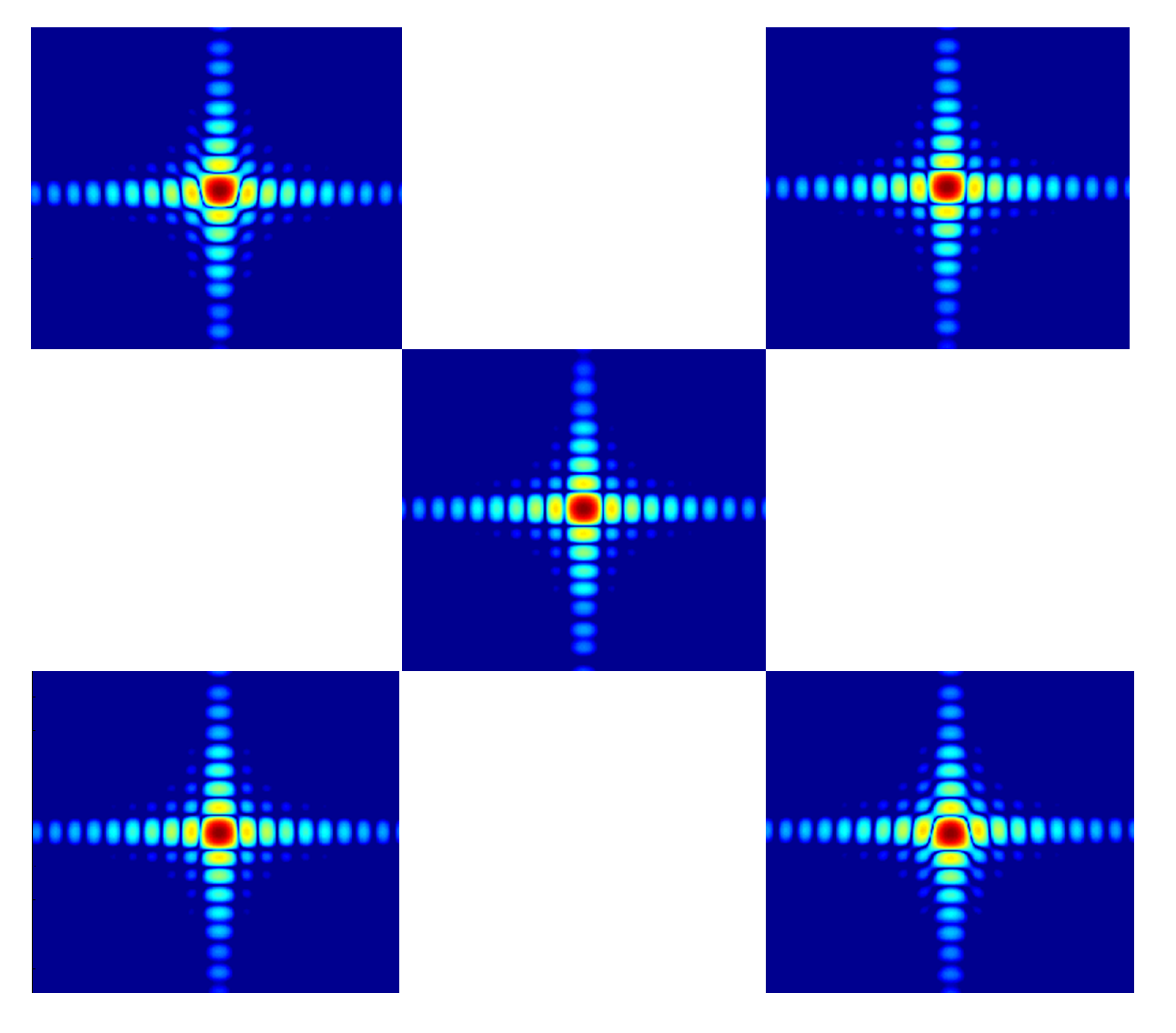
Imaging experiments with an orbit-inclined GEO SAR system were carried out to validate the algorithm proposed in Section 4, the systematic parameters of which are listed in Table 3. A scene with a size of 20 km × 20 km is fixed near the Equator, and 25 points are uniformly distributed as a dot-matrix in it with the neighboring intervals of 4.5 km × 4.5 km, which is shown in Figure 12. In the imaging experiments, two typical BTD error cases are considered, where the main component of Case 1 is quadratic and that of Case 2 is cubic. The 3D shapes of BTD errors are plotted in Figure 13, in which the meteorological parameters of the edges (A, B, C, D) and center (E) are listed in Table 4. Thus, considering the two cases of BTD errors, two different raw data of GEO SAR are generated. Further, four different imaging results are achieved with or without the compensation of BTD error, i.e., Case 1 without BTD compensation, Case 1 with BTD compensation, Case 2 without BTD compensation, and Case 2 with BTD compensation. Five points (four edge points and the central point in Figure 12) are selected to show the details of the imaging results. The 2D focused image of the points in the dB scale are plotted in Figure 14, Figure 15, Figure 16 and Figure 17, and the imaging quality of point targets is counted and listed in Table 5. For Case 1, the main component is quadratic, just as expected, and an obvious main lobe expansion in the azimuth direction can be detected when comparing Figure 14 and Figure 15. Similarly, an asymmetric sidelobe appears in Case 2 with the cubic main component. Comparing the imaging qualities without and with BTD compensation, it can be concluded that the proposed algorithm can well compensate the decorrelation caused by the BTD error.
With the support of the external data sources of the meteorological parameters and the SAR systematic parameters, the proposed algorithm can be introduced into the existing SAR signal processing to improve the SAR image formation module and reduce the influence of BTD. For the future advanced SAR survey, the proposed algorithm can be used directly as the image formation module with the functions of BTD and spatial variation compensations.
6. Summary
The effect of BTD error is considered in this paper. First, we discuss and model the decorrelation problems introduced by SAR geometry and BTD error. Second, in the framework of GEO SAR geometry, BTD error is divided into constant error, spatially variant error, and time variant error, and the influences are analyzed respectively. It is concluded that constant error and spatially variant error are very weak in GEO SAR imaging and could be ignored, while the influence of time variant error should be considered. Third, considering the influences of spatial variation, BTD error, and the cross-coupling between them, an imaging algorithm is proposed to achieve a better focusing depth. Finally, the imaging experiments demonstrate that the proposed algorithm can well process the main lobe expansion and asymmetric sidelobe problems caused by BTD error, and a well-focused image is achieved after the decorrelation compensation.
Author Contributions
Conceptualization, D.L.; methodology, D.L., X.Z., Z.D., A.Y., and Y.Z.; software, D.L. and A.Y.; validation, D.L. and Z.D.; formal analysis, D.L. and Y.Z.; investigation, D.L., X.Z., and A.Y.; resources, Z.D. and Y.Z.; supervision, D.L., Z.D., and Y.Z.; validation, D.L.; writing, review and editing, D.L. All authors have read and agreed to the published version of the manuscript.
Funding
This research was funded by the National Natural Science Foundation of China under Grant Number 61771478.
Acknowledgments
The authors are grateful for the anonymous reviewers for their valuable suggestions.
Conflicts of Interest
The authors declare no conflict of interest. The funders had no role in the design of the study; in the collection, analyses, or interpretation of data; in the writing of the manuscript; nor in the decision to publish the results.
References
- Rodon, J.R.; Broquetas, A.; Guarnieri, A.M.; Rocca, F. Geosynchronous SAR Focusing with Atmospheric Phase Screen Retrieval and Compensation. IEEE Trans. Geosci. Remote Sens. 2013, 51, 4397–4404. [Google Scholar] [CrossRef]
- Tomiyasu, K. Synthetic aperture radar in geosynchronous orbit. In Proceedings of the Synthetic Aperture Radar Technology Conference, Washington, DC, USA, 15–19 March 1978. [Google Scholar]
- Kou, L.; Xiang, M.; Wang, X.; Zhu, M. Tropospheric effects on L-band geosynchronous circular SAR imaging. IET Radar Sonar Navig. 2013, 7, 693–701. [Google Scholar] [CrossRef]
- Hobbs, S.E.; Guarnieri, A.M.; Broquetas, A.; Calvet, J.C.; Casagli, N.; Chini, M.; Ferretti, R.; Nagler, T.; Pierdicca, N.; Prudhomme, C.; et al. G-CLASS: Geosynchronous radar for water cycle science— Orbit selection and system design. J. Eng. 2019, 21, 7534–7537. [Google Scholar] [CrossRef]
- Hanssen, R. Radar Interferometry: Data Interpretation and Error Analysis; Kluwer: Dordrecht, The Netherlands, 2001. [Google Scholar]
- Li, D.; Dong, Z.; Yu, A.; Zhang, Y.; Zhang, Q.; He, F.; Wu, M. Estimation and Compensation of turbulent tropospheric delay in High-resolution SAR Image. IEEE Trans. Geosci. Remote Sens. 2020. [Google Scholar] [CrossRef]
- Ji, Y.; Zhang, Q.; Zhang, Y.; Dong, Z.; Yao, B. Spaceborne P-band SAR imaging degradation by anisotropic ionospheric irregularities: A comprehensive numerical study. IEEE Trans. Geosci. Remote Sens. 2020, 58, 5516–5526. [Google Scholar] [CrossRef]
- Ji, Y.; Zhang, Y.; Dong, Z.; Zhang, Q.; Li, D.; Yao, B. Impacts of ionospheric irregularities on L-band geosynchronous synthetic aperture radar. IEEE Trans. Geosci. Remote Sens. 2020, 58, 3941–3954. [Google Scholar] [CrossRef]
- Ishimaru, A.; Kuga, Y.; Liu, J.; Kim, Y.; Freeman, T. Ionospheric effects on synthetic aperture radar at 100 MHz to 2 GHz. Radio Sci. 1999, 34, 257–268. [Google Scholar] [CrossRef]
- Breit, H.; Fritz, T.; Balss, U.; Lachaise, M.; Niedermeier, A.; Vonavka, M. TerraSAR-X SAR Processing and Products. IEEE Trans. Geosci. Remote Sens. 2010, 48, 727–740. [Google Scholar] [CrossRef]
- Prats-Iraola, P.; Scheiber, R.; Rodriguez-Cassola, M.; Mittermayer, J.; Wollstadt, S.; Zan, F.D.; Bräutigam, B.; Schwerdt, M.; Reigber, A.; Moreira, A. On the Processing of Very High Resolution Spaceborne SAR Data. IEEE Trans. Geosci. Remote Sens. 2014, 52, 6003–6016. [Google Scholar] [CrossRef] [Green Version]
- Yu, Z.; Li, Z.; Wang, S. An imaging compensation algorithm for correcting the impact of tropospheric delay on spaceborne high-resolution SAR. IEEE Trans. Geosci. Remote Sens. 2015, 53, 4825–4836. [Google Scholar] [CrossRef]
- Guarnieri, A.M.; Leanza, A.; Recchia, A.; Tebaldini, S.; Venuti, G. Atmospheric Phase Screen in GEO-SAR:Estimation and Compensation. IEEE Trans. Geosci. Remote Sens. 2018, 56, 1668–1679. [Google Scholar] [CrossRef]
- Saastamoinen, J. Atmospheric correction for the troposphere and stratospherein radio ranging of satellites. Geophys. Monogr. Ser. 1972, 15, 247–251. [Google Scholar]
- Davis, J.L.; Herring, T.A.; Shapiro, I.I.; Rogers, A.E.E.; Elgered, G. Geodesy by radio interferometry: Effects of atmospheric modeling errors on estimates of baseline length. Radio Sci. 1985, 20, 1593–1607. [Google Scholar] [CrossRef]
- Askne, J.; Nordius, H. Estimation of tropospheric delay for microwaves from surface weather data. Radio Sci. 1987, 22, 379–386. [Google Scholar] [CrossRef]
- Böhm, J.; Werl, B.; Schuh, H. Troposphere mapping functions for GPS and very long baseline interferometry from European Centre for Medium-Range Weather Forecasts operational analysis data. J. Geophys. Res. 2006, 111. [Google Scholar] [CrossRef]
- Rasmussen, C.E.; Williams, C.K. Gaussian Processes for Machine Learning; The MIT Press: Cambridge, MA, USA, 2006. [Google Scholar]
- George, W.K. Lectures in Turbulence for the 21st Century; Imperial College of London: London, UK, 2013. [Google Scholar]
- Li, D.; Rodriguez-Cassola, M.; Prats-Iraola, P.; Dong, Z.; Wu, M.; Moreira, A. Modeling of Tropospheric Delays in Geosynchronous Synthetic Aperture Radar. China Sci. Inform. Sci. 2017, 60, 81–98. [Google Scholar] [CrossRef]
- Hu, C.; Liu, Z.; Long, T. An Improved CS Algorithm Based on the Curved Trajectory in Geosynchronous SAR. IEEE J. Sel. Top. Appl. Earth Obs. Remote Sens. 2012, 5, 795–808. [Google Scholar] [CrossRef]
- Sun, G.C.; Xing, M.; Wang, Y.; Yang, J.; Bao, Z. A 2-D Space-Variant Chirp Scaling Algorithm Based on the RCM Equalization and Subband Synthesis to Process Geosynchronous SAR Data. IEEE Tran. Geosci. Remote Sens. 2014, 52, 4868–4880. [Google Scholar]
- Li, D.; Wu, M.; Sun, Z.; He, F.; Dong, Z. Modeling and Processing of Two-Dimensional Spatial-Variant Geosynchronous SAR Data. IEEE J. Sel. Topics Appl. Earth Observ. Remote Sens. 2015, 8, 3999–4009. [Google Scholar] [CrossRef]
- Wong, F.H.; Cumming, I.G.; Neo, Y.L. Focusing Bistatic SAR Data Using the Nonlinear Chirp Scaling Algorithm. IEEE Trans. Geosci. Remote Sens. 2008, 46, 2493–2505. [Google Scholar] [CrossRef] [Green Version]
- Smith, E.K.; Weintraub, S. The Constants in the Equation for Atmospheric Refractive Index at Radio Frequencies. Proc. IRE 1953, 41, 1035–1037. [Google Scholar] [CrossRef] [Green Version]
- Boehm, J.; Heinkelmann, R.; Schuh, H. Short Note: A global model of pressure and temperature for geodetic applications. J. Geod. 2007, 81, 679–683. [Google Scholar] [CrossRef]
- Lagler, K.; Schindelegger, M.; Boehm, J.; Krásná, H.; Nilsson, T. GPT2: Empirical slant delay model for radio space geodetic techniques. Geophys. Res. Lett. 2013, 40, 1069–1073. [Google Scholar] [CrossRef] [PubMed] [Green Version]
- Böhm, J.; Möller, G.; Schindelegger, M.; Pain, G.; Weber, R. Development of an improved empirical model for slant delays in the troposphere (GPT2w). GPS Solut. 2015, 19, 433–441. [Google Scholar] [CrossRef] [Green Version]
- Cumming, I.G.; Wong, F.H. Digital Processing of Synthetic Aperture Radar; Artech House: Boston, MA, USA, 2005. [Google Scholar]
Figure 1.
(a) Tropospheric propagation within SAR acquisition geometry. (b) The block diagram of the tropospheric delay model. BTD, background tropospheric delay; GPT2w, global pressure and temperature 2 wet; ZHD, zenith hydrostatic delay; ZWD, zenith wet delay; TTD, turbulent tropospheric delay; STD, slant tropospheric delay.

Figure 2.
Division of the BTD error.

Figure 3.
(a) Variation of ZHD with the pressure and temperature. (b) Variation of ZWD with the temperature and water vapor pressure.
Figure 3.
(a) Variation of ZHD with the pressure and temperature. (b) Variation of ZWD with the temperature and water vapor pressure.
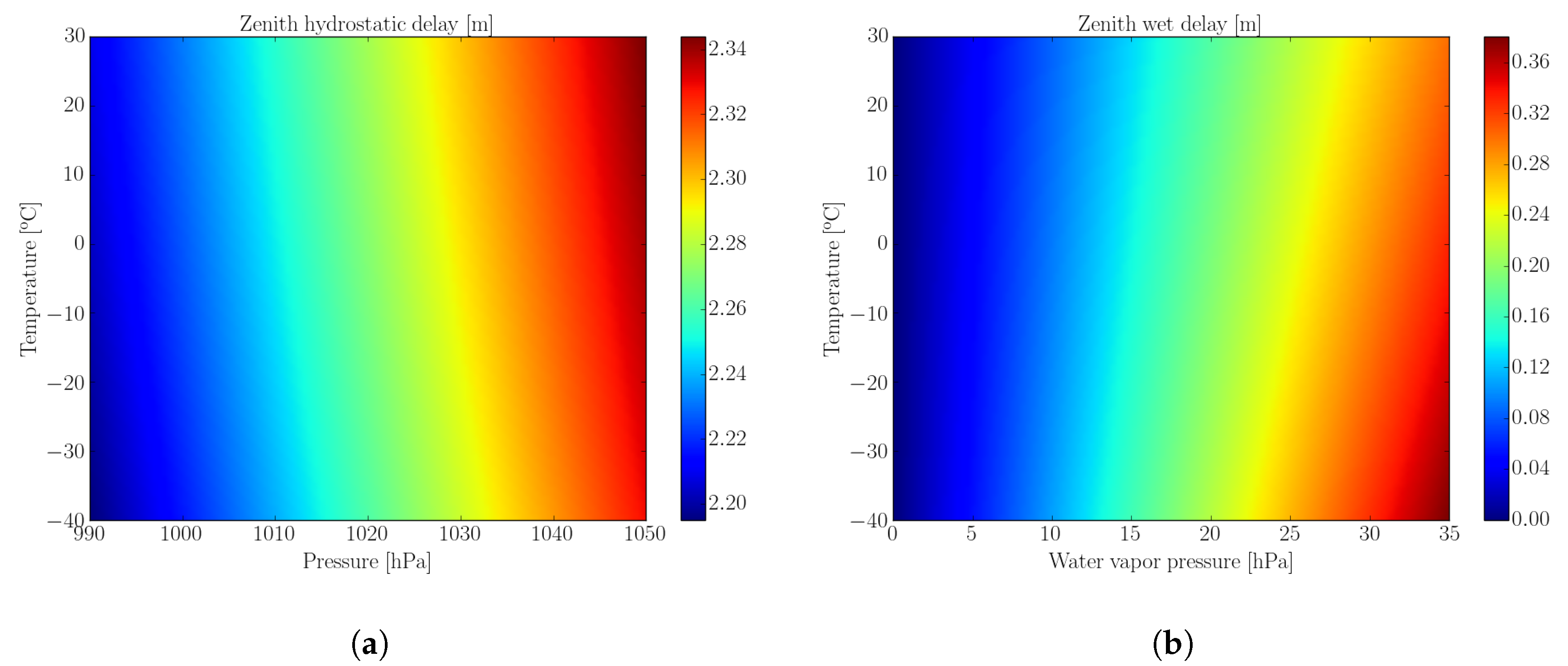
Figure 4.
Bias of ZHD along with the variation of the pressure (a) and temperature (b).
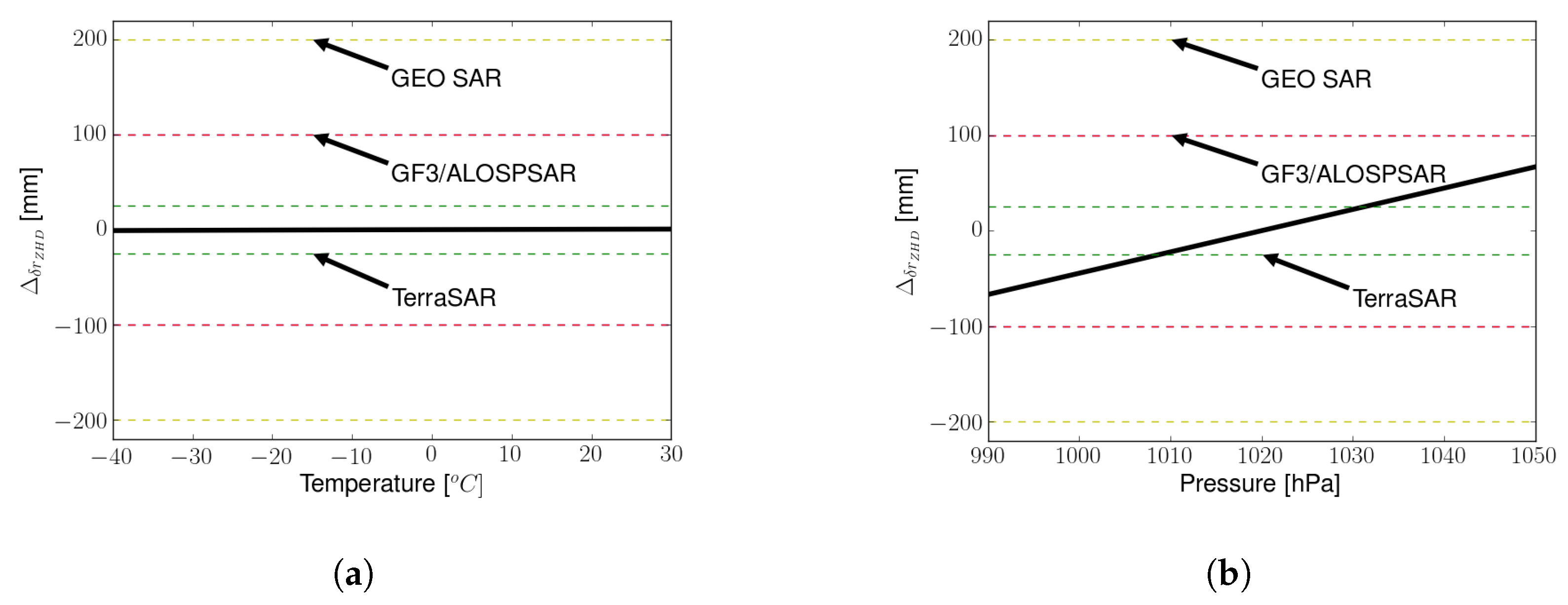
Figure 5.
Bias of ZWD along with the variation of the temperature (a) and water vapor pressure (b).
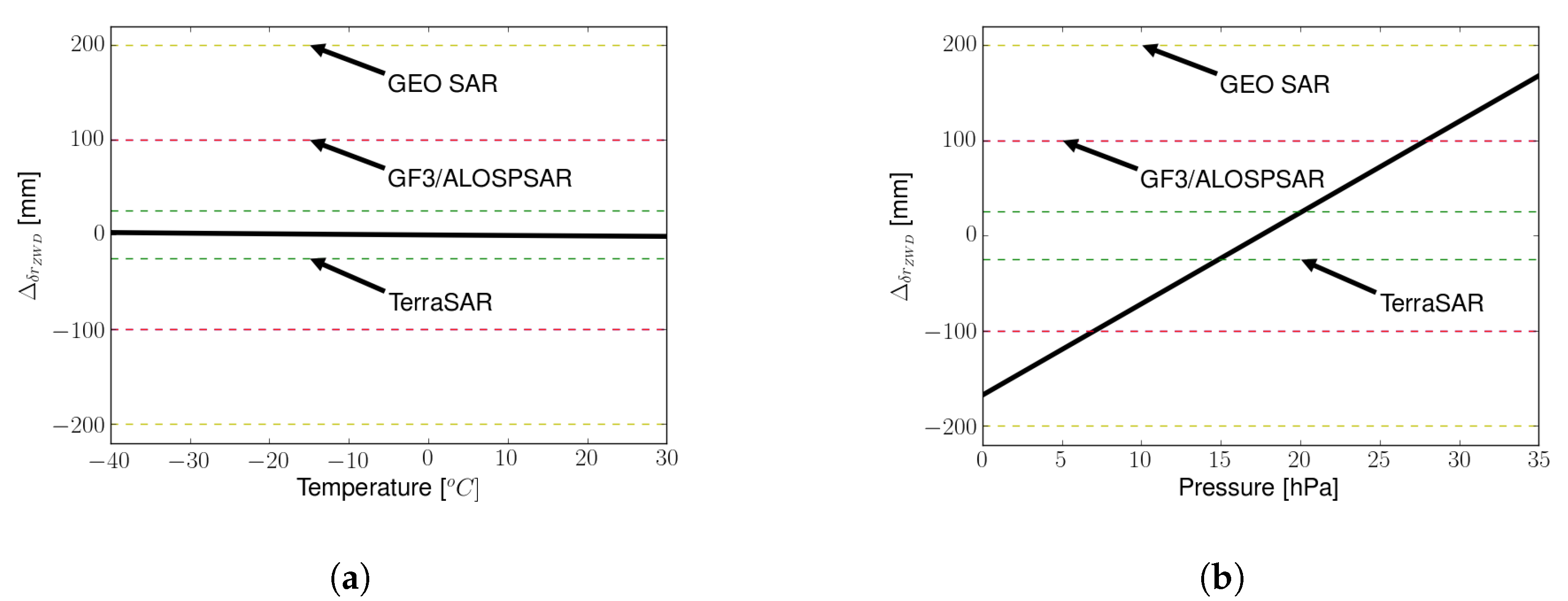
Figure 6.
Influences of the spatially variant error of BTD on the azimuth impulse response under different integration times in the X band (a), C band (b), and L band (c) cases. The blue dotted line represents the ideal result, and the red solid line represents the influenced result.
Figure 6.
Influences of the spatially variant error of BTD on the azimuth impulse response under different integration times in the X band (a), C band (b), and L band (c) cases. The blue dotted line represents the ideal result, and the red solid line represents the influenced result.
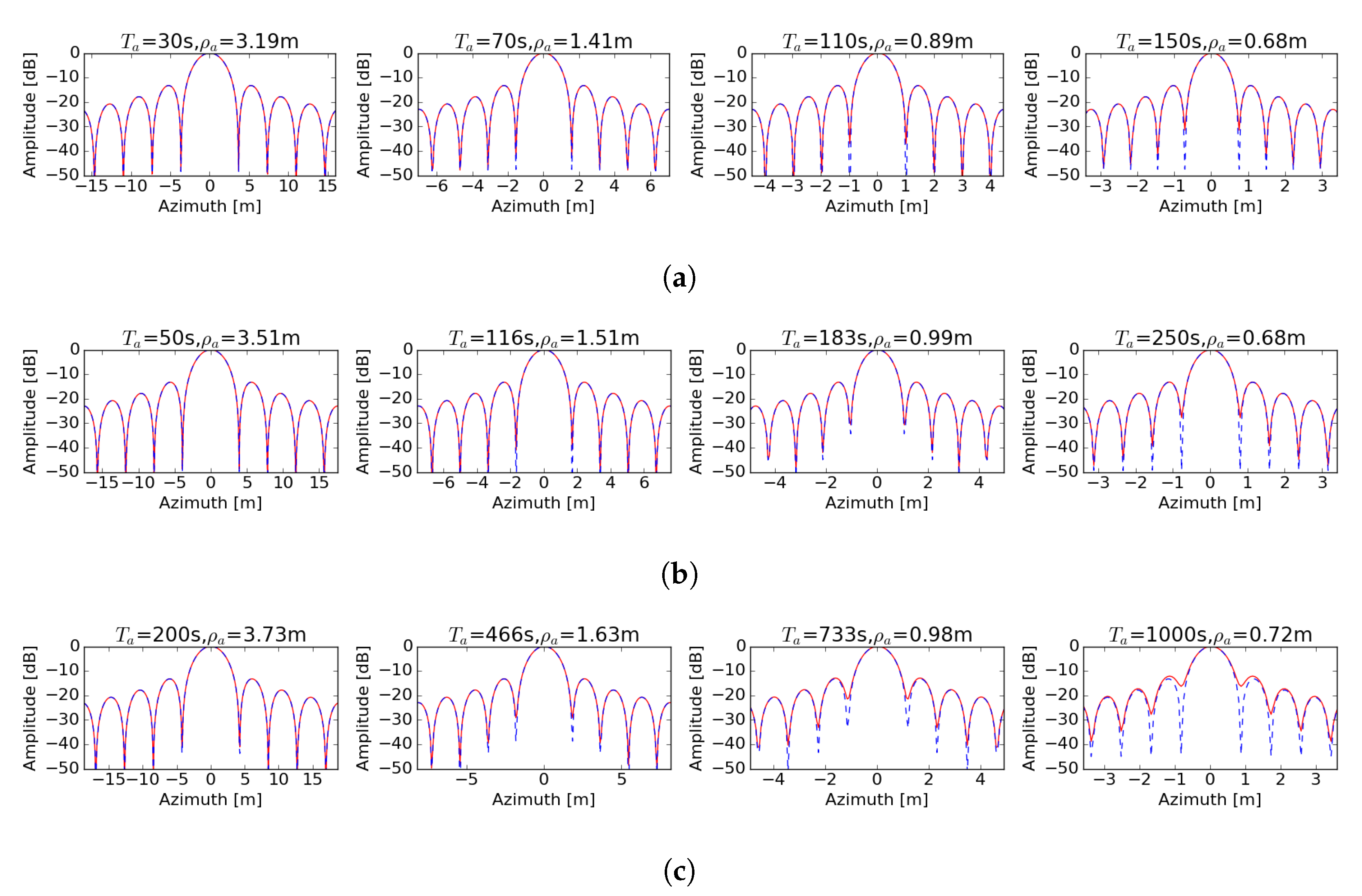
Figure 7.
Typical cases of the time variant error of BTD (linear variation, quadratic variation, and cubic variation).
Figure 7.
Typical cases of the time variant error of BTD (linear variation, quadratic variation, and cubic variation).

Figure 8.
Influences of time variant error on the azimuth impulse response under different integration times with the X band: (a) Case 0, (b) Case 1, and (c) Case 2. The blue dotted line represents the ideal result, and the red solid line represents the influenced result.
Figure 8.
Influences of time variant error on the azimuth impulse response under different integration times with the X band: (a) Case 0, (b) Case 1, and (c) Case 2. The blue dotted line represents the ideal result, and the red solid line represents the influenced result.
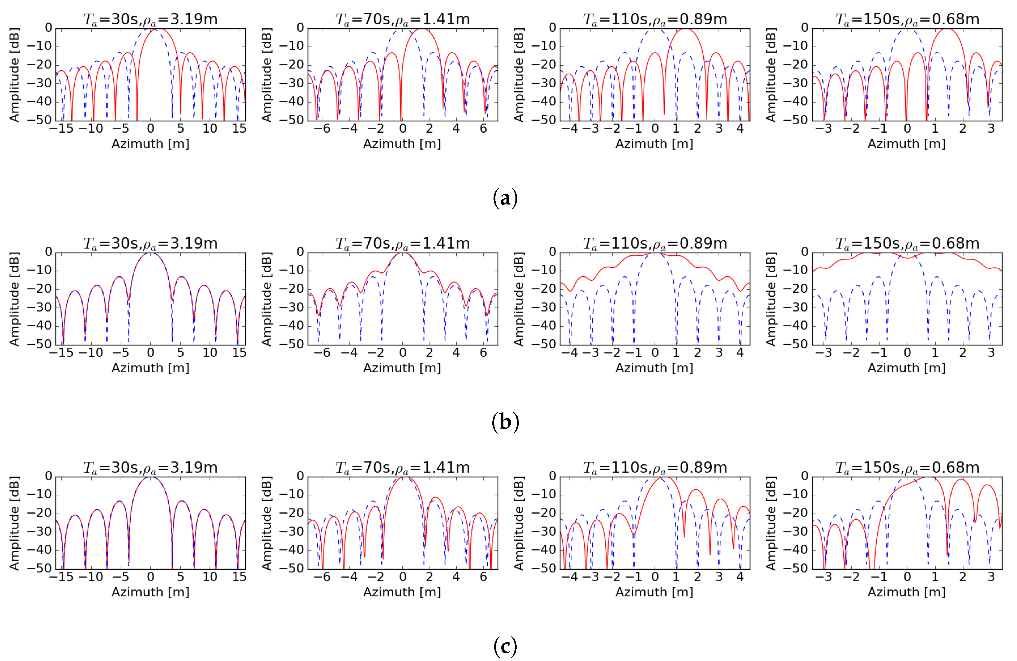
Figure 9.
Influences of the time variant error on the azimuth impulse response under different integration times with the L band: (a) Case 0, (b) Case 1, and (c) Case 2. The blue dotted line represents the ideal result, and the red solid line represents the influenced result.
Figure 9.
Influences of the time variant error on the azimuth impulse response under different integration times with the L band: (a) Case 0, (b) Case 1, and (c) Case 2. The blue dotted line represents the ideal result, and the red solid line represents the influenced result.
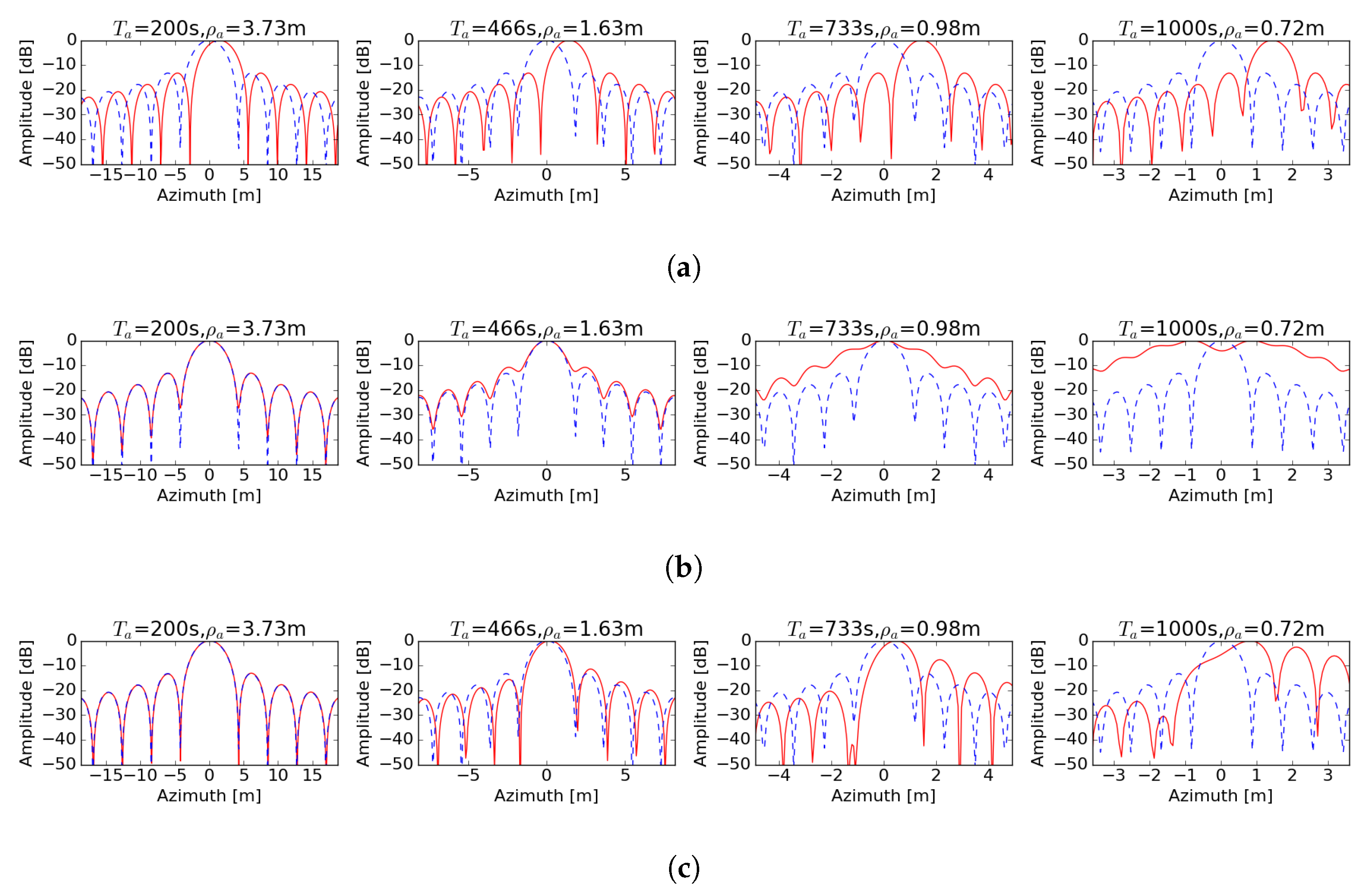
Figure 10.
2D spatially variant geometry model of GEO SAR imaging.

Figure 11.
2D spatially variant geometry model of GEO SAR imaging.

Figure 12.
Point target distribution in the scene.
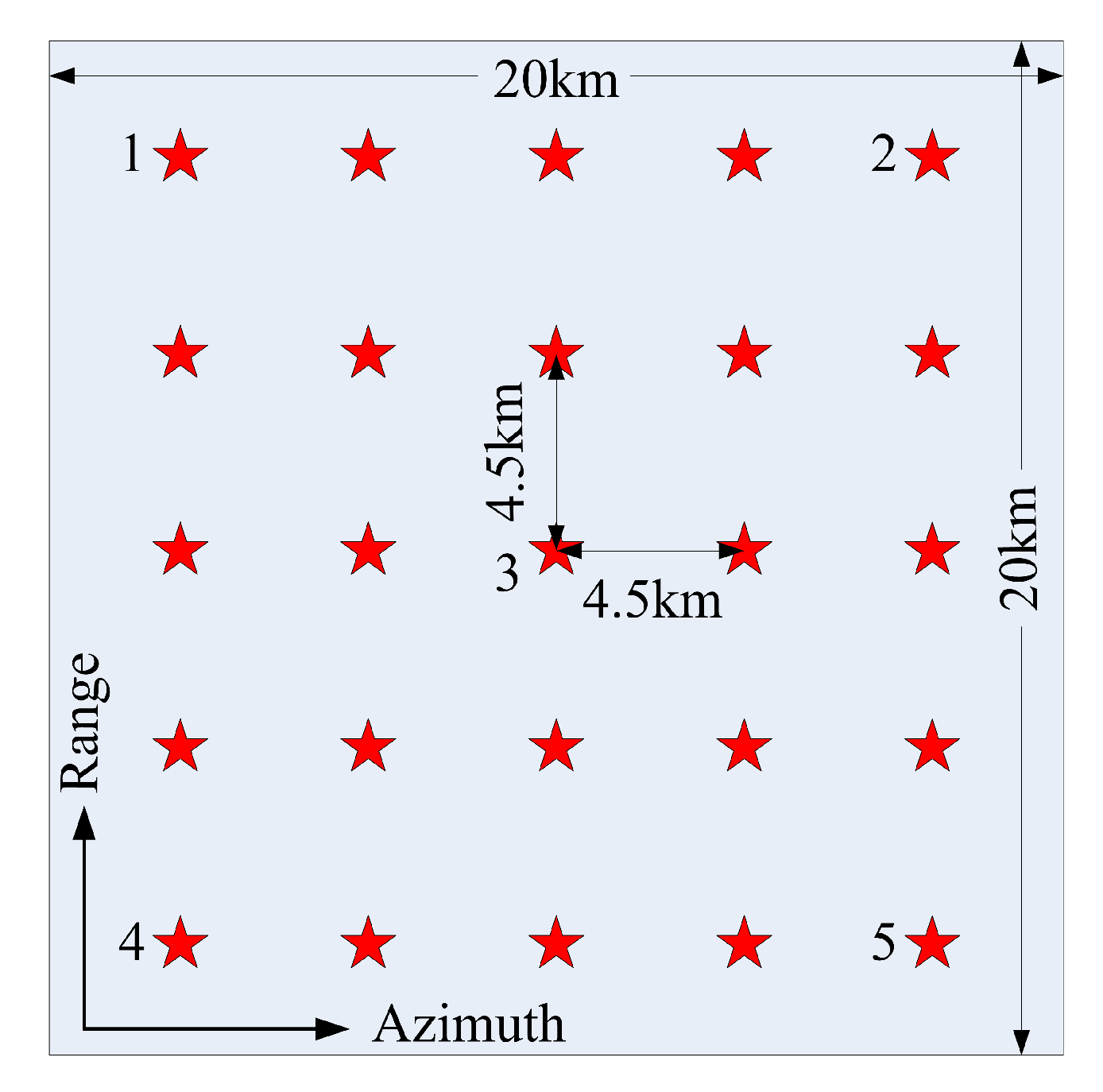
Figure 13.
Two typical BTD errors for the GEO SAR imaging simulation. (a) Case 1: the main component is quadratic. (b) Case 2: the main component is cubic.
Figure 13.
Two typical BTD errors for the GEO SAR imaging simulation. (a) Case 1: the main component is quadratic. (b) Case 2: the main component is cubic.

Figure 14.
Imaging results of Case 1 without the BTD error compensation.

Figure 15.
Imaging results of Case 1 with the BTD error compensation.

Figure 16.
Imaging results of Case 2 without the BTD error compensation.
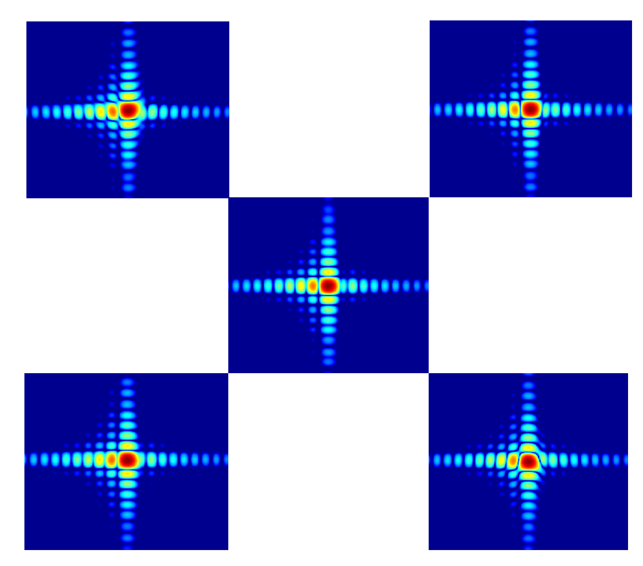
Figure 17.
Imaging results of Case 2 with the BTD error compensation.

Table 1.
Parameters for Vienna mapping functions.
| Parameters | Values | Parameters | Values |
|---|---|---|---|
| 0.0029 | 0.062 | ||
| (, 0) | (0.007, 0.005) | ||
| (0.002, 0.001) | 0.0000253 | ||
| 0.00549 | 0.00114 | ||
| 0.00146 | 0.04391 |
Table 2.
Systematic parameters of typical spaceborne SAR.
| Parameters (Units) | TerraSAR | ALOS-PSAR | GF3 | GEO SAR |
|---|---|---|---|---|
| Orbital height (km) | 514 | 691.65 | 755 | 36,000 |
| Eccentricity (-) | 0 | 0 | 0 | 0 |
| Orbital inclination (deg) | 97.44 | 98.16 | 97 | 60 |
| Incident angle (deg) | 15∼60 | 8∼60 | 10∼60 | 25 |
| Antenna size (m × m) | 0.7 × 4.78 | 3.1 × 8.9 | 1.5 × 15 | 30 × 30 |
| Waveband | X | L | C | L |
Table 3.
Systematic parameters of GEO SAR configurations.
| Parameters | Values | Units |
|---|---|---|
| Semi-major axis | 42,164.17 | km |
| Eccentricity | 1 × 10⁻⁸ | |
| Orbital inclination | 60 | deg |
| Right ascension of ascending (RAAN) | 0 | deg |
| Perigee | 0 | deg |
| True anomaly | 0 | deg |
| Carrier frequency | 1.25 | GHz |
| Antenna size | 30 × 30 | m × m |
| Squint angle | 0 | deg |
| Incident angle | 30.28 | deg |
| Pulse repetition frequency (PRF) | 200 | Hz |
| Chirp duration | 1 | s |
| Chirp bandwidth | 30 | MHz |
Table 4.
The meteorological parameters of BTD errors.
| Cases | Point | A | B | C | D | E |
|---|---|---|---|---|---|---|
| Case 1 | 1008.1 | 1008.44 | 1008.4 | 1008.92 | 1009.29 | |
| 28 | 29.5 | 30 | 29 | 30 | ||
| 5.79 | 8.59 | 8.6 | 11.38 | 22.95 | ||
| Case 2 | 1008.1 | 1008.44 | 1008.47 | 1009.29 | 1008.9 | |
| 28 | 29.5 | 29 | 30 | 29.3 | ||
| 5.79 | 14.28 | 14.26 | 22.95 | 17.21 |
Table 5.
The imaging quality of point targets.
| Targets | 1 | 2 | 3 | 4 | 5 | ||||||
|---|---|---|---|---|---|---|---|---|---|---|---|
| Cases | Azimuth | Range | Azimuth | Range | Azimuth | Range | Azimuth | Range | Azimuth | Range | |
| Case 1 without BTD compensation | IRW | 2.14 | 4.44 | 2.10 | 4.41 | 2.14 | 4.45 | 2.13 | 4.41 | 2.12 | 4.45 |
| PSLR | −8.95 | −14.23 | −8.88 | −13.99 | −8.32 | −13.85 | −8.96 | −13.90 | −8.60 | −13.90 | |
| ISLR | −6.21 | −11.09 | −7.22 | −10.96 | −6.20 | −10.60 | −6.22 | −10.88 | −6.96 | −10.83 | |
| Case 1 with BTD compensation | IRW | 2.04 | 4.45 | 2.03 | 4.45 | 2.04 | 4.41 | 2.04 | 4.45 | 2.04 | 4.48 |
| PSLR | −13.06 | −13.89 | −13.22 | −13.71 | −13.26 | −14.07 | −13.25 | −13.72 | −13.14 | −13.90 | |
| ISLR | −9.78 | −10.93 | −9.77 | −10.74 | −9.84 | −10.98 | −9.89 | −10.69 | −9.81 | −10.82 | |
| Case 2 without BTD compensation | IRW | 2.08 | 4.47 | 2.04 | 4.45 | 2.06 | 4.41 | 2.09 | 4.47 | 2.05 | 4.48 |
| PSLR | −8.48 | −13.95 | −9.48 | −13.71 | −9.07 | −14.08 | −8.47 | −13.72 | −9.40 | −13.90 | |
| ISLR | −12.21 | −10.93 | −12.97 | −10.74 | −12.99 | −10.96 | −12.28 | −10.67 | −13.31 | −10.81 | |
| Case 2 with BTD compensation | IRW | 2.04 | 4.47 | 2.04 | 4.45 | 2.04 | 4.41 | 2.05 | 4.45 | 2.04 | 4.48 |
| PSLR | −13.05 | −13.90 | −13.19 | −13.71 | −13.27 | −14.07 | −13.21 | −13.72 | −13.12 | −13.90 | |
| ISLR | −9.71 | −10.93 | −9.82 | −10.74 | −9.85 | −10.98 | −9.85 | −10.70 | −9.90 | −10.82 | |
Note: IRW, impulse response width; PSLR, peak side lobe ratio; ISLR, integral side lobe ratio.
© 2020 by the authors. Licensee MDPI, Basel, Switzerland. This article is an open access article distributed under the terms and conditions of the Creative Commons Attribution (CC BY) license (http://creativecommons.org/licenses/by/4.0/).
Share and Cite
MDPI and ACS Style
Li, D.; Zhu, X.; Dong, Z.; Yu, A.; Zhang, Y. Background Tropospheric Delay in Geosynchronous Synthetic Aperture Radar. Remote Sens. 2020, 12, 3081. https://doi.org/10.3390/rs12183081
AMA Style
Li D, Zhu X, Dong Z, Yu A, Zhang Y. Background Tropospheric Delay in Geosynchronous Synthetic Aperture Radar. Remote Sensing. 2020; 12(18):3081. https://doi.org/10.3390/rs12183081
Chicago/Turabian StyleLi, Dexin, Xiaoxiang Zhu, Zhen Dong, Anxi Yu, and Yongsheng Zhang. 2020. "Background Tropospheric Delay in Geosynchronous Synthetic Aperture Radar" Remote Sensing 12, no. 18: 3081. https://doi.org/10.3390/rs12183081
Note that from the first issue of 2016, this journal uses article numbers instead of page numbers. See further details here.