Topological Space Knowledge Distillation for Compact Road Extraction in Optical Remote Sensing Images

1
Aerospace Information Research Institute, Chinese Academy of Sciences, Beijing 100190, China
2
Key Laboratory of Network Information System Technology (NIST), Aerospace Information Research Institute, Chinese Academy of Sciences, Beijing 100190, China
3
University of Chinese Academy of Sciences, Beijing 100190, China
4
School of Electronic, Electrical and Communication Engineering, University of Chinese Academy of Sciences, Beijing 100190, China
*
Author to whom correspondence should be addressed.
Remote Sens. 2020, 12(19), 3175; https://doi.org/10.3390/rs12193175
Submission received: 22 August 2020
/
Revised: 21 September 2020
/
Accepted: 23 September 2020
/
Published: 28 September 2020
(This article belongs to the Special Issue Remote Sensing for Urban Development and Sustainability)
Abstract
:Road extraction from optical remote sensing images has drawn much attention in recent decades and has a wide range of applications. Most of the previous studies rarely take into account the unique topological characteristics of the road. It is the most apparent feature of linear structure that describes the variety of connection relationships of the road. However, designing a particular topological feature extraction network usually results in a model that is too heavy and impractical. To address the problems mentioned above, in this paper, we propose a lightweight topological space network for road extraction based on knowledge distillation (TSKD-Road). Specifically, (1) narrow and short roads easily influence topological features extracted directly in optical remote sensing images. Therefore, we propose a denser teacher network for extracting road structures; (2) to enhance the weight of topological features, we propose a topological space loss calculation model with multiple widths and depths; (3) based on the above innovations, a topological space knowledge distillation framework is proposed, which aims to transfer different kinds of knowledge acquired in a heavy net to a lightweight net, while significantly improving the lightweight net’s accuracy. Experiments were conducted on two publicly available benchmark datasets, which show the obvious superiority and effectiveness of our network.
1. Introduction
Road extraction in remote sensing images is always a research hotspot for its wide applications, such as in navigation [1], map updating [2], disaster detection [3,4,5], and so on. Especially with the development of intelligent transportation, it is of considerable significance to develop not only high accuracy, but also compact methods for road extraction.
In the past few decades, road extractions have mainly been based on handcrafted features, such as road color, geometry, spectral characteristics, and so on. Lue et al. [6] used the spectral difference between roads and others to extract road pixels. Ghaziani, M. et al. [7] utilized the segmentation method, which set several thresholds based on statistical road features, to achieve the binary classification of road and non-road. Hao Chen et al. [8] proposed the fusion of prior topological the road data with a road skeleton to obtain high-accuracy road extraction. These methods play a significant role in the performance improvement of road extraction. However, due to the strong dependence on handcrafted features, they have poor performance in robustness and generalization, especially for images with complicated backgrounds.
Recently, due to the automatic learning abilities of modeling feature expression, many deep- learning-based methods have been proposed for road extraction in remote sensing images. The research on road extraction based on deep learning is mainly divided into two stages. The first stage mainly introduces the existing deep learning segmentation network into road extraction. These methods mostly rely on convolutional neural networks (CNNs) and fully convolutional neural networks (FCNs) [9]. Mnih and Hinton et al. [10] first applied deep learning methods to road extraction tasks. They employed restricted Boltzmann machines to segment roads based on patch images. In 2018, the D-LinkNet network proposed by Lichen Zhou et al. [11] won the championship of the DeepGlobe Road Extraction Challenge [12]. This method increases the network reception domain, retains the spatial details of the road, and effectively improves the road’s recognition accuracy. The above methods can obtain high-order features of and information on the road, which increases the power of handling road scene variations and deep semantic information. However, the characteristics of the road itself have rarely been introduced. For example, the centerline and boundary features of roads can be regarded as the other two forms of roads. In addition, humans usually follow the road in a specific direction, so the direction information is also a kind of road feature. In addition, topological features are also unique features of roads. The above features can better summarize the road characteristics, but such features are rarely used in the methods mentioned above.
In the second stage, researchers try to extract and detect features that match the characteristics of road targets in remote sensing images based on existing networks. Therefore, more road characteristics are added, such as direction information [13,14], centerline and edge of the road [15,16,17,18], and topological features. As for the topological features, Hu Xiaoling et al. [19] achieved both per-pixel accuracy and topological correctness with an end-to-end deep segmentation network. They put forward a topological loss that forces the segmentation results to have the same Betti number (number of connected components and handles) as the ground truth. Because the matching process needs to compute the Betti number, the computation of topological information is relatively expensive. Mosinska et al. [20] proposed the use of a pre-trained VGG19 net to construct a topological space loss. Although promising performance was achieved, their model still suffered from two drawbacks. The first problem is that the above method does not take into account the different forms of road connectivity or the typical topological structures. As shown in Figure 1, there are three classical topological structures: bifurcated structures, cruciform structures, and ring structures. They all have multiple connected components and decentralized structures in which the feature pixels of the road in the optical remote sensing image are scattered in position. They are different from other cluster features, such as buildings, airplanes, and so on, which is the main feature of linear structures like roads. However, the above methods use image patches as the input of the network; thus, it is difficult for the network to extract different forms of topological structures if the receptive field is too small. Another problem is that to extract the topology and achieve high accuracy, they usually design complex and heavy networks, requiring extensive computing resources and memory consumption. However, for example, in the case of flood [3], tsunami, earthquake [4], and landslide [5] disaster relief efforts, they all desire live drone imagery of the damaged roads. Therefore, it would bring more benefits if segmentation efficiency could be further improved. Moreover, when on-the-ground analysis of newly acquired images is required, this would require the use of smaller GPUs embedded into a laptop, implying significant memory constraints. To conclude, there is a need for a simple, lightweight road topological loss solution to improve the segmentation efficiency and reduce limitations by the capacity of available hardware (GPU and memory-wise).
In order to simplify the network structure, a lot of research on lightweight networks has recently appeared, such as mobilenet [21] and shufflenet [22], which have simple network structures and require little in terms of computing resources. However, applying them directly to road extraction will achieve low accuracy and rough extraction results. Recently, a method that can combine the high precision of complex networks and the light weight of compact networks has emerged, which is knowledge distillation. Knowledge distillation is an effective method to achieve a lightweight network with considerable accuracy. As can be seen in Figure 2a,b, compared with the ordinary network, knowledge distillation aims at transferring knowledge acquired in one model (teacher net, which is heavy but has high accuracy) to another model (student net, which is light but has low accuracy) without requiring any special operators while getting enhanced generalization. In 2014, Rich Caruana et al. [23] proposed that the shallow model imitates the behavior of the deep model and achieves considerable accuracy. In 2015, Hinton et al. [24] formally proposed the concept of knowledge distillation, which has been applied in many fields, including classification [25], object detection [26], semantic segmentation [27], and so on. W. Park et al. [28] proposed relational knowledge distillation, which can transmit interrelated data instances. It uses the distance-wise and angle-wise distillation losses to compensate for the structural differences of the relationship between different pixels. Especially in metric learning, it allows students to outperform teachers’ performance. Liu Y. et al. [27] proposed the use of three distillation methods: pixel distillation, pair-wise distillation, and structural distillation (GAN) in semantic segmentation, which focused on the three different aspects of distillation (pixel, pair relationship, structure) and achieved outstanding segmentation results. Knowledge distillation provides new insights into model compression, which lets us know that a lightweight network can achieve better performance.
In this work, to better utilize the topological structures of roads and improve the accuracy and efficiency in road extraction, we propose a topological space distillation method, which does not need to redesign or match a topological loss function, but also solves the problem of complex and heavy networks. As can be seen in Figure 2c, it distills two kinds of knowledge from the teacher network: the widely used pixel-level feature distillation and a new kind of structure-level knowledge, which is also called the topological space feature. It can achieve the migration of topological space features from a teacher network to a lightweight network. Therefore, it can help the lightweight network summarize the topological information of surrounding pixels and pay attention to key areas, such as intersections. By introducing this, the network can achieve more continuous road detection results.
The main contributions can be summarized as the following:
- A topological space knowledge distillation model named TSKD-Road is proposed for road extraction in remote sensing images. Our framework achieves high accuracy on a lightweight network. Compared with the state-of-art networks, TSKD-Road has fewer parameters and achieved considerable road detection accuracy. To the best of our knowledge, it is the first attempt to combine knowledge distillation with road extraction.
- To enhance the weight of topological features, inspired by [29], we apply a topological space loss calculation model (TSKD) to train a lightweight topological integrity framework, which is based on knowledge distillation. The new topological space model can help the network achieve more consistent road detection results.
- To better extract topological features of the road, a robust and dense encoder–decoder teacher network (D-EDTN) is designed. The network could better recover more detailed spatial information on roads that are too short or too narrow. Therefore, the network can better collect more topological features and improve network accuracy.
2. Materials and Methods
In this section, our proposed method for road extraction is discussed in detail. This section consists of four main parts. The first part is the overview of the whole network, which describes in detail the composition of our method. The second part is the pre-distillation part, which is used to output the prediction score map and transpose the pixel-based knowledge from the teacher net to the student net. The third part is the post-distillation part, which generates topological space loss and transposes the teacher net’s structure-based knowledge to the student net. The last part is all the loss functions used in TSKD-Road.
2.1. Overview of the Whole Method
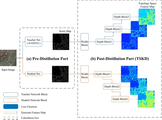
The common distillation method is mostly based on the output of the teacher network. For example, as can be seen in Figure 2b, the basic knowledge distillation method is mostly distilling the prediction output of the network. In order to let students learn more road features from the network, other than the pre-distillation part, the post-distillation model is applied, which not only allows the student network to learn more generalized topological features, but also ensures the model’s light weight. Figure 3 shows the detailed configuration of the proposed method, which mainly includes two parts: the pre-distillation part and the post-distillation part. The pre-distillation part is a kind of pixel-level distillation, and the post-distillation part is the structure-level distillation. The remote sensing image is first input into the pre-distillation part to get the prediction (score maps). Then, the score map is input into the post-distillation part for assisting the pre-distillation part in extracting topological space information.
To realize a lightweight road extraction student network, we choose the lightweight MobileNetV2 as the backbone, which is used as a student network in knowledge distillation. Moreover, the teacher network output is used to guide the student network so that the knowledge learned by the teacher net can be transferred to the student network. The above process is the pre-distillation. What is more, to better extract the topological structure of the road, we designed a more powerful teacher net (D-EDTN) that could better extract the details of narrow and short roads. In addition, a robust teacher model yields a proportional increase in the accuracy of the student model, which also means that a stronger teacher network can teach a better student network; when the accuracy of the teacher network increases, the accuracy of the student network will also improve.
The common pixel-based loss function has the limitation that it only calculates the difference between the corresponding pixels without considering the overall structure. To extract different forms of road features, especially topological features, and increase the amount of knowledge transferred from the teacher network to the student network, we designed the post-distillation stage using the road topology characteristics learned by the teacher network to guide the output of the student network. So, the student network has not only the supervision of the pixel layer, but also the overall supervision. This post-distillation is also named the topological space knowledge distillation part (TSKD). The input of this part is the output of the teacher net and student net. Its outputs are the multi-width and multi-depth feature maps of topological space.
Taking into account the analysis as mentioned above, we propose a new kind of distillation framework for road extraction. The entire method can be reformulated in Algorithm 1.
| Algorithm 1 Topological space network for road extraction based on knowledge distillation (TSKD-Road). |
| Input: The RGB remote sensing image ; The corresponding ground-truth labeling y, where ; |
| Output: Student network model, and the road segmentation results; |
| 1: step1: pre-distillation |
| 2: Extract the prediction segmentation results by the teacher net (D-EDTN) and the student net ; |
| 3: Calculate the semantic segmentation loss ; |
| 4: Calculate the pre-distillation loss ; |
| 5: step2: post-distillation |
| 6: Normalize and ; |
| 7: Extract features and by the width TSKD; |
| 8: Initialize = 0; |
| 9: for do |
| 10: ; |
| 11: Calculate the post-distillation loss = + (, ); |
| 12: end for |
2.2. Pre-Distillation Part
To effectively extract narrow and short roads, we propose the use of a dense encoder–decoder teacher network (D-EDTN) to guide the lightweight student net, which is the pre-distillation process.
2.2.1. Dense Encoder–Decoder Teacher Network (D-EDTN)
For the task of road extraction, it is hard to get both the high-resolution features and rich semantic information. Furthermore, in remote sensing images, a large part of the road looks short and narrow. The urban branch roads and rural roads have fewer pixels in width, and there are many short roads in the communities of cities. In multiple downsampling operations, semantic information became wealthy, but the location information was reduced a lot. Thus, it has a strong desire for high-resolution spatial information. The encoder–decoder network D-LinkNet has achieved high computational efficiency, but a simple encoder–decoder module cannot satisfy the extraction requirements. Although the multi-stage series–parallel atrous convolution increases the receptive field, it cannot solve the problem of the loss of spatial information caused by multiple downsampling, especially for images with lower resolution. The detailed feature information of the road is complete in the high-resolution layer. As a result, rather than restore high resolution from low resolution, we choose to keep high resolution with more encoder and decoder blocks.
As can be seen in Figure 4, the network uses ResNet34 pre-trained on an ImageNet dataset as its encoder: e00, e10, e20, e30, and e40. The input size of the net is pixels of each image. Thus, the output size of each feature layer is 256 pixels, 128 pixels, 64 pixels, or 32 pixels. For the decoder block: d31, d22, d13, d16, and d01; Figure 4a shows the details. It has two convolutions, and one transposed convolution with the stride of 2; m is the input channel size, and n is the out channel size. The output of each horizontal line is at the same size.
To better obtain the semantic information of the high-resolution layers, six blue blocks, e11, e12, e21, d14, d15, and d23, called High-Resolution Blocks (HRBs), as shown in Figure 4b, are added; here, m is the input channel size, and n is the out channel size. In addition, except for the addition operation from encoder block to decoder block, as shown in the figure in orange skip lines, more concatenation operations are added to assist the HRBs in recovering the semantic information of the high resolution, as shown in the figure with the blue skip dotted connections.
We formulate the six blocks as follows: Let denote the encoder block of the three blue circles in Figure 4, and represents the three blue decoder blocks, where i indexes the same down-sampling layer and j indexes the convolution layer of the net.
where function is the convolution operation, like in Figure 4a. means the up-sampling to the same size as the ith layer. denotes the concatenation layer, and + is the addition operation. D represents the output feature of the Dblock. Here, the e in Equation (1) is the e in Equation (2); therefore, we make full use of the HRB in the decoder block. The decoder block not only relies on the low-resolution layer, but also the same resolution layer to get more detailed information. Therefore, the net can efficiently extract the narrow and short roads that are similar to the background or have small loops. The above two equations show how feature maps travel through the dense net.
2.2.2. The Lightweight Student Network
In order to train a lightweight model and reduce memory, the backbone of the student net we choose is the MobileNetV2, which is based on Depthwise Separable Convolutions [30]. The entire student net is composed of seven basic blocks, M1, M2, ..., M7, as can be seen in Figure 5. Each basic block is a linear bottleneck depthwise separable convolution with residuals, which significantly reduces the memory requirement and prevents nonlinearities from destroying too much information. Moreover, rather than directly getting the final feature maps from M7, the M3 and a coarse bilinear interpolation upsampling of M7 are fused to combine the low-level spatial road information with abundant high-level semantic features.
2.3. Post-Distillation Part
To extract topological road features and improve the student net’s accuracy, we design a simple but efficient framework called the topological space knowledge distillation model (TSKD). It can help the network acquire multidimensional topological structures from several convolutional layers.
The detailed framework of the TSKD is presented in Figure 6. On the one hand, for extracting multi-width topological features, the width-TSKD is designed. Rather than actually resampling features, the multiple parallel atrous convolutional layers are combined with different rates to effectively capture multi-scale information. This includes: (a) one convolution and three convolutions with rates = (6, 12, 18) (all with 32 channels and batch normalization that follows), and (b) the image-level features. The above structure resembles the Atrous Spatial Pyramid Pooling (ASPP) module [31]; the difference is that, in order to certainly reduce computational burden and achieve translation invariance over small spatial shifts in the image, as well as to expand the receptive field, four max-pooling layers with a pixel filter are added after the atrous convolutional layer. By combining the multi-scaled local receptive field and global information of topological structures efficiently and flexibly, the width-TSKD can capture multi-scaled feature layers.
On the other hand, for extracting multi-depth topological features, one convolution and three convolutional layers are added after the width-TSKD. Here, a convolutional layer with nonlinear units follows. These convolutions are applied to generalize different dimensions and sizes of topological space features. The output feature size of each convolutional layer is , and . Consequently, the three convolutional layers make up the high-level semantic features of topological space that might be missing from the common distillation. Meanwhile, combining multiple intermediate features at different scales contributes to improving the road extraction results.
The TSKD module tries to obtain higher-order semantic information of the road topology. This includes some key points of bifurcated structures, road connectivity, and clear edges with accurate holes. To verify our method’s effectiveness, we visualized the output of the last three convolutional layers, which is also the output of three width-TSKD blocks. This can be seen in Figure 7. The three images on the upper right are the output from the teacher net, and the corresponding three images below are the output from the student net. With the increase of the width-TSKD block, the topological features of the roads are extracted well. We noticed from the figure that the topological characteristics of the teacher network’s output are more evident and prominent. Compared with the student net’s outputs, the road lines are more visible, the area of the road is more precise, and more bifurcated structures are concerned. Then, by reducing the error between the output feature maps of the student net and the teacher net, the topological features can be better transferred from the teacher net to the student net.
2.4. Loss Function of TSKD-Road
The composition of the entire loss is shown below, which consists of three parts: the segmentation part, the pre-distillation part, and the post-distillation part, as shown in Figure 3.
Given RGB remote sensing imagery as the input, we get the output . Let y be the ground truth label. Each y and is the pixel i of the image.
Sematic segmentation loss: The road extraction is a primary semantic segmentation task. We use the binary cross-entropy loss. Due to the unbalanced samples of road and background, we add the SoftIoU loss [32].
Pre-distillation loss: Knowledge distillation aims to transform more information from the teacher net to student net. Thus, we apply two different kinds of strategies in the pre-distillation part.
One is pixel-wise distillation. The student net learns and fits the output of the teacher net pixel by pixel. The form of the loss function is the Kullback–Leibler divergence, defined as:
where and stands for the outputs from the last layers of the student net and teacher net.
The other is pair-wise distillation, which can help the student net learn a similarity-preserving knowledge distillation. For example, similar (dissimilar) output in the teacher network will produce similar (dissimilar) activation in the student net. The form of the loss function adopted is the mean squared error loss, which can be denoted as:
where and represent the similarity between pixel i and pixel j of the student net and teacher net, which can be simply computed from the features and as:
Because the framework of the teacher net and the student net are entirely different, the above two distillation strategies are only used in the last output layer of the networks.
Post-distillation loss: The post-distillation loss tries to minimize the differences between what the teacher net describes in the three feature maps’ topological space and what the corresponding student net describes, which is introduced by Mosinska et al. [28].
where N represents three feature maps, n=1,2,3. C represents the channels of each feature map. R represents each pixel of the feature map. and represent the outputs of the teacher net and student net. Such an operation allows us to increase the depth and width of the high-dimension topological space. In other words, by minimizing this loss, the student net can better learn a function of the teacher net to extract the topological space.
3. Experiments
In this section, to demonstrate the effectiveness of the proposed method, extensive experiments were conducted based on two well-known publicly available road extraction datasets. Concerning comparative evaluation, we adopted some well-known methods as baselines.
3.1. Datasets
3.1.1. Massachusetts Roads Dataset
This dataset [10] consists of 1171 aerial images. The training set, test set, and validation set are split into 1108 images, 49 images, and 14 images. Each image is pixels in size, covering an area of 2.25 square kilometers. The resolution is 1 m/pixel. The whole dataset covers over 2600 square kilometers, including urban, suburban, and rural regions. Such a complex background has various topological structures, which can be used to evaluate the efficiency of our method and make the road extraction extremely challenging.
3.1.2. RoadNet Dataset
This dataset is from [18]. The dataset consists of 20 aerial images. The training set and test set are split into 14 images and 6 images. It covers 21 regions, about 8 square kilometers. They are all from Ottawa, Canada. The resolution is m/pixel. This is five times the resolution of the Massachusetts Roads Dataset, so it can effectively detect our method’s adaptability to high-resolution images.
3.2. Experimental Setting
All the methods in this paper were implemented with Google colab, based on a K80GPU (with 12 GB GPU memory). The “polynomial” learning rate (with power = 0.9) policy was employed for all the experiments. The learning rate was originally set to 2 × 10. Data augmentation is adopted on both datasets to avoid overfitting. Three common kinds of flips are used: horizontal, vertical, and diagonal, and uncommon color jittering is added as well. The last step is image shifting and scaling.
For the Massachusetts Roads Dataset, since all the images in the Massachusetts Roads Dataset are pixels, to adapt to the receptive field in this method, we resize all the images to pixels for adapting our network. For the RoadNet Dataset, because each image’s size is different, we crop the image into the same size, pixels with a step of 512 pixels. Thus, the training and test sets are made up of 918 images and 192 images, respectively.
3.3. Evaluation Metrics
We employed the six most common metrics for evaluating road extraction results, including the parameters (to calculate the number of network parameters during testing), the inference time (Infer Time) of each image patch with a size of pixels on the K80GPU (with 12 GB GPU memory), recall, precision, F1 score, mIoU, and Road IoU. Precision measures the true pixels of the road in all the predicted pixels of road, and recall represents the ratio of predicted pixels of the road to all the true pixels of the road. F1 score and mIoU are the comprehensive evaluation indexes. Road IoU is also a comprehensive metric, which is for the road class only. The above four metrics are calculated as follows:
Here, TP, TN, FN, and FP denote the count of true positives, the count of true negatives, the count of false negatives, and the count of false positives, respectively.
3.4. Ablation Study
We conducted ablation studies on the Massachusetts dataset, considering that it has over 2600 square kilometers and covers three regions: urban, rural, and suburban. It could fully evaluate the ability to deform various kinds of roads with a diverse background.
3.4.1. Comparison of the Dense Encoder–Decoder Teacher Network (D-EDTN)
To compare the performance of our proposed D-EDTN with the baseline D-LinkNet, we report the results in Figure 8 and Table 1. From the visual results in Figure 8, it can be seen that D-LinkNet had high performance due to its substantial center dilation part that expanded the receptive field of convolution. However, it still can not pay attention to the short and narrow roads; with our proposed method, this problem is alleviated. The D-EDTN shows more short and narrow roads in Figure 8c compared with the baseline D-LinkNet in Figure 8b. The D-EDTN establishes more contact between encoder and decoder, especially in high resolution, which helps the net obtain detailed semantic information to recover the short and narrow roads.
The first two rows of Table 1 show the quantitative comparison of our method with D-LinkNet. The segmentation performance was evaluated using six different feature descriptors: Road IoU, mIoU, F1 score, recall, precision, parameters, and Infer Time. These show that our proposed method achieves slight improvements compared with the D-LinkNet; the F1 score, mIOU, and Road IoU are respectively increased by 1.28%, 0.88%, and 1.64%, while the Infer Time and the parameters just increased by 60.1 ms and 0.7 MB. With such a strong teacher net, the student net can be trained better and can extract more topological space features.
3.4.2. Comparison of Different Kinds of Knowledge Distillation on the Student Net
In this comparative experiment, we applied different kinds of knowledge distillation strategies on the lightweight network. As shown in Figure 9, the middle feature results of three images were displayed, which are all from the M7 feature map of the student net. From left to right, each column is the image, the result of student net, the result of common knowledge distillation, the result of D-EDTN distillation, the result of TSKD, and the label. It can be seen in Figure 9b that the student net gets weak semantic information, and the features of the road cannot be well noticed. In Figure 9c,d, some regions are activated. Especially with the application of D-EDTN, some short and narrow roads are noticed. When applying the TSKD, the features of the roads are gathered together and shown more continuously. In particular, from Figure 9e, it can be seen that the road not only has strong semantic information, but the method also starts to pay attention to the topological information of the road where it has cruciform structures and bifurcated structures.
As seen in the outputs of the different methods shown in Figure 10, the student net performs better and better with the application of knowledge distillation. The basic lightweight net without distillation misses many roads. From Figure 10c, it is clear to see that the student net with knowledge distillation captures more information than before. Apart from this, with the dense encoder–decoder teacher net (D-EDTN), the student yields better results. This is attributed to our dense model, which can get more detailed information about the narrow and short roads. This also verified the effectiveness of the proposed teacher net in contributing to the student net’s learning more spatial information about the unique scaled road. What is more, by integrating the topological space knowledge distillation (TSKD), the results are the best of all, demonstrating that the topological loss based on distillation is suitable for the road extraction task. As we shall see, with the topological loss, the student net produces a more consistent result, no matter if the roads are long or short.
To quantitatively assess the knowledge distillation performances of the proposed method, we list the quantitative comparison in the last four rows of Table 1. The metrics for evaluation are Road IoU, mIoU, F1 score, recall, precision, parameters, and Infer Time. Compared with the previously mentioned teacher net, the parameters of the student net are only 3.25 M, and the Infer Time is 33.5 ms, which are all the smallest and almost ten times smaller than those of the teacher net. The performance of the teacher net (D-EDTN) and student net (TSKD) can also be seen in Figure 11a. The student net shows a balanced performance between the parameters and the accuracy. Although it is only one-tenth of the parameter amount of the teacher network, it can still exhibit similar accuracy performance. As for Road IoU, mIoU, and F1 score, as shown in Figure 11b, with the distillation, the student net outperforms the baseline by 0.82%, 0.46%, and 0.70%. When applying the multi-scaled teacher net to the distillation (D-EDTN KD), it outperforms by 1.90%, 1.03%, and 1.57%, whereas with the TSKD, it outperforms by 2.59%, 1.39%, and 2.13%, which are consistent with our visual judgment.
Therefore, the results mentioned above demonstrated that the knowledge distillation and topological space loss could effectively help the lightweight network achieve higher accuracy without increasing any parameters or models of the lightweight network.
3.5. Comparison with the State-of-the-Art Methods
To evaluate the effectiveness of the proposed method (TSKD-Road), we compared with different recent state-of-the-art road extraction methods, including DeepLab-v3, PSPNet, ENet, D-LinkNet, and RoadNet, and also compared the most relevant topology model, Mosinska’s method.
3.5.1. Results with the Massachusetts Dataset
Figure 12 shows the visualized results of the Massachusetts Dataset. It can be seen that our proposed method generally performs better than the baseline methods. The RoadNet, ENet, Mosinska, and PSPNet methods miss road regions and over-extracted in some places, especially for roads in which spectral characteristics are very similar to surrounding features, while the deeplab-v3 generally performs better, but a few discontinuities still exist. The D-LinkNet misses some roads when the roads are too narrow. Compared with all the baseline methods, our method learns more high-resolution semantic information and topological features of the road from the teacher network, which remarkably improved its fitting and understanding ability. As can be seen in Figure 13, for some small and narrow roads in the image, our network can effectively extract these parts of the roads and supplement the complete topology of the roads.
Table 2 presents the comparative quantitative results measured in terms of Road IoU, mIoU metrics, F1 score, recall, precision, parameters, and Infer Time. It can be seen from the table that our method has fewer parameters and lower Infer Time (compared with PSPNet, Deeplab-v3, RoadNet, and D-LinkNet), which are more than 5–20 times less than with those methods. This brings more possibilities for use in mobile computation. What is more, for the F1 score, Road IoU, and mIoU, our method tends to yield the best performance. In order to better show the difference between Mosinska‘s method and our net, Table 3 lists the comparison in terms of Road IoU, mIoU metrics, F1 score, topo-parameters, and whether a pre-trained model is used. Here, the topo-parameters indicate the number of topological network parameters. We use the same main network, MobilenetV2, to compare the differences in the topological networks. It can be seen that our topological network is more than 20 times smaller than Mosinska‘s. We do not need to use a pre-trained network, which makes the training process lighter and does not require storage of huge parameters of the model. More importantly, our method shows better performance in accuracy of Road IoU, mIoU, and F1 score.
3.5.2. Results with the RoadNet Dataset
In this subsection, we evaluate our method when used on the RoadNet Dataset. It is a high-resolution dataset and has many shadow-occluded areas, which brings challenges to our method. This can test the adaptability of our network to different resolutions. A visual comparison between the extraction results is shown in Figure 14. We can see from the figure that our method achieved a more promising performance than the other methods. Figure 14b shows that there are serious “salt and pepper” phenomena and wrong segmentation in Deeplabv3, while the ENet, RoadNet, Mosinska’s method, and PSPNet in Figure 14c–f improved a lot in this regard. However, these methods are likely to over-extract and have rough edges. Among all the methods, D-LinkNet and our method have smoother edges and performed better. However, the D-LinkNet shows some false positive parts. In summary, compared with the above methods, our method shows more completeness of the road, which means that our proposed TSKD model can capture the road’s topological characteristics. Meanwhile, Figure 15 shows the detailed segmentation results of our network. We can see that the underlying topological structure of the road is segmented clearly, especially for the shadow occlusion area. It can be seen in the four enlarged parts of the image that our network can overcome this problem and get the smooth road edges. The above results show that our method can effectively extract the topological structure of the road and overcome the non-obvious road features caused by environmental factors, such as tree shadows.
Table 4 shows the quantitative results compared with different methods. Our method yields the fewest parameters (3.25 M) and lowest Infer Time (33.5 ms) compared with Deeplab-v3, RoadNet, PSPNet, Mosinska, and D-LinkNet. Moreover, our method shows better results compared with Deeplab-v3, RoadNet, PSPNet, Mosinska, and ENet. In general, this method has achieved a relatively balanced performance between accuracy and parameters.
4. Discussion
We present our analysis and discussion in this section. The topological features of the road are used in this paper to enhance the ability of our network. In order not to increase the parameters of the network and to avoid the complicated topological loss calculation model, we adopted the knowledge distillation method. Knowledge distillation not only does not need to design a particular topological feature extraction network, but can also solve the problem of heavy models. It can be seen from Section 3 that our method has made great progress on two datasets.
In terms of the first dataset with low-resolution imagery, it is vital to get the high-resolution features, which have rich spatial information. In conditions in which low-resolution images have few pixels on small roads and multiple down-sampling operations easily lose position information, we designed the dense encoder–decoder teacher network (D-EDTN) structure to focus the position information in the pre-distillation stage. As can be seen in Figure 12 and Figure 13, our method has shown excellent extraction capabilities in areas where road features are not obvious, as well as where roads are small and narrow.
In terms of the second dataset with high-resolution imagery, which has a lot of shadow occlusion areas, it is vital to focus on the broken segmentation road results. Therefore, the topological space loss calculation model (TSKD) we designed in the post-distillation stage is used to extract the topological characteristics of the road and, at the same time, to restore the areas occluded by shadows. It can be seen in Figure 14 and Figure 15 that our method can get a relatively complete road structure, which means that the topological characteristics we extracted are more consistent with the labeling.
Finally, we also compared many methods using parameters of the networks and the Infer Time. As can be seen in Table 1 and Figure 11, our method can obtain a lightweight model while retaining a certain accuracy rate. Compared with our baseline model (D-LinkNet), our parameters and Infer Time are both reduced by about ten times. We can also see in Table 2 and Table 4 that our method keeps a balance between accuracy and Infer Time.
However, our proposed method could not get delicate information about the edges of roads due to the lightweight network itself and the way of knowledge distillation. We will leave it for future work to incorporate sufficient semantic information and different kinds of knowledge distillation to extract roads well.
5. Conclusions
In this paper, a high-accuracy and lightweight topological space network based on knowledge distillation is proposed for road extraction. The two knowledge distillation methods, pre-distillation and post-distillation, can dramatically improve the accuracy of the lightweight network while maintaining the computing power and parameters of the network. The pre-distillation can especially pay attention to small and narrow roads, and the post-distillation provides a specific topological space distillation model for road extraction that can produce more continuous roads. Extensive experiments verify the advantages of our method, which achieves not only a light weight, but also performs better than state-of-the-art methods. To the best of our knowledge, this is the first time that such a lightweight but high-accuracy network has been trained for road extraction. In summary, this research sheds new light on road extraction based on a lightweight network. In future work, we will pay more attention to extracting more smooth road edges to make the model more accurate.
Author Contributions
Formal analysis, K.G.; Funding acquisition, X.S., Z.Y., W.D., and X.G.; Investigation, K.G.; Methodology, K.G.; Supervision, X.S., Z.Y., W.D., and X.G.; Visualization, K.G.; Writing—original draft, K.G.; Writing—review and editing, K.G., X.S., Z.Y., W.D., and X.G. All authors have read and agreed to the published version of the manuscript.
Funding
This work is supported by the National Natural Science Foundation of China under Grants 41701508 and 61725105.
Conflicts of Interest
The authors declare no conflict of interest.
References
- Li, Q.; Chen, L.; Li, M.; Shaw, S.L.; Nüchter, A. A sensor-fusion drivable-region and lane-detection system for autonomous vehicle navigation in challenging road scenarios. IEEE Trans. Veh. Technol. 2013, 63, 540–555. [Google Scholar] [CrossRef]
- Bonnefon, R.; Dhérété, P.; Desachy, J. Geographic information system updating using remote sensing images. Pattern Recognit. Lett. 2002, 23, 1073–1083. [Google Scholar] [CrossRef]
- Ahmad, K.; Pogorelov, K.; Riegler, M.; Ostroukhova, O.; Halvorsen, P.; Conci, N.; Dahyot, R. Automatic detection of passable roads after floods in remote sensed and social media data. Signal Process. Image Commun. 2019, 74, 110–118. [Google Scholar] [CrossRef] [Green Version]
- Coulibaly, I.; Spiric, N.; Sghaier, M.O.; Manzo-Vargas, W.; Lepage, R.; St-Jacques, M. Road extraction from high resolution remote sensing image using multiresolution in case of major disaster. In Proceedings of the 2014 IEEE Geoscience and Remote Sensing Symposium, Quebec City, QC, Canada, 13–18 July 2014; pp. 2712–2715. [Google Scholar]
- Liu, C.; Li, W.; Lei, W.; Liu, L.; Wu, H. Architecture planning and geo-disasters assessment mapping of landslide by using airborne LiDAR data and UAV images. In Proceedings of the International Symposium on Lidar and Radar Mapping 2011: Technologies and Applications. International Society for Optics and Photonics, Nanjing, China, 26–29 May 2011; Volume 8286, p. 82861Q. [Google Scholar]
- Lu, P.; Du, K.; Yu, W.; Wang, R.; Deng, Y.; Balz, T. A new region growing-based method for road network extraction and its application on different resolution SAR images. IEEE J. Sel. Top. Appl. Earth Obs. Remote Sens. 2014, 7, 4772–4783. [Google Scholar] [CrossRef]
- Ghaziani, M.; Mohamadi, Y.; Koku, A.B.; Konukseven, E.I. Extraction of unstructured roads from satellite images using binary image segmentation. In Proceedings of the 2013 21st Signal Processing and Communications Applications Conference (SIU), Haspolat, Turkey, 24–26 April 2013; pp. 1–4. [Google Scholar]
- Chen, H.; Yin, L.; Ma, L. Research on road information extraction from high resolution imagery based on global precedence. In Proceedings of the 2014 Third International Workshop on Earth Observation and Remote Sensing Applications (EORSA), Changsha, China, 11–14 June 2014; pp. 151–155. [Google Scholar]
- Long, J.; Shelhamer, E.; Darrell, T. Fully convolutional networks for semantic segmentation. In Proceedings of the IEEE Conference on Computer Vision and Pattern Recognition, Boston, MA, USA, 7–12 June 2015; pp. 3431–3440. [Google Scholar]
- Mnih, V.; Hinton, G.E. Learning to detect roads in high-resolution aerial images. In Lecture Notes in Computer Science, Proceedings of the European Conference on Computer Vision, Heraklion, Crete, Greece, 5–11 September 2010; Springer: Berlin/Heidelberg, Germany, 2010; pp. 210–223. [Google Scholar]
- Zhou, L.; Zhang, C.; Wu, M. D-LinkNet: LinkNet With Pretrained Encoder and Dilated Convolution for High Resolution Satellite Imagery Road Extraction. In Proceedings of the ICVPR Workshops, Salt Lake City, UT, USA, 18–22 June 2018; pp. 182–186. [Google Scholar]
- Demir, I.; Koperski, K.; Lindenbaum, D.; Pang, G.; Huang, J.; Basu, S.; Hughes, F.; Tuia, D.; Raska, R. Deepglobe 2018: A challenge to parse the earth through satellite images. In Proceedings of the 2018 IEEE/CVF Conference on Computer Vision and Pattern Recognition Workshops (CVPRW), Salt Lake City, UT, USA, 18–22 June 2018; pp. 172–17209. [Google Scholar]
- Batra, A.; Singh, S.; Pang, G.; Basu, S.; Jawahar, C.; Paluri, M. Improved road connectivity by joint learning of orientation and segmentation. In Proceedings of the IEEE Conference on Computer Vision and Pattern Recognition, Long Beach, CA, USA, 15–21 June 2019; pp. 10385–10393. [Google Scholar]
- Bastani, F.; He, S.; Abbar, S.; Alizadeh, M.; Balakrishnan, H.; Chawla, S.; Madden, S.; DeWitt, D. Roadtracer: Automatic extraction of road networks from aerial images. In Proceedings of the IEEE Conference on Computer Vision and Pattern Recognition, Salt Lake City, UT, USA, 18–22 June 2018; pp. 4720–4728. [Google Scholar]
- Cheng, G.; Wang, Y.; Xu, S.; Wang, H.; Xiang, S.; Pan, C. Automatic road detection and centerline extraction via cascaded end-to-end convolutional neural network. IEEE Trans. Geosci. Remote Sens. 2017, 55, 3322–3337. [Google Scholar] [CrossRef]
- Lu, X.; Zhong, Y.; Zheng, Z.; Liu, Y.; Zhao, J.; Ma, A.; Yang, J. Multi-Scale and Multi-Task Deep Learning Framework for Automatic Road Extraction. IEEE Trans. Geosci. Remote Sens. 2019, 57, 9362–9377. [Google Scholar] [CrossRef]
- Yang, X.; Li, X.; Ye, Y.; Lau, R.Y.; Zhang, X.; Huang, X. Road Detection and Centerline Extraction Via Deep Recurrent Convolutional Neural Network U-Net. IEEE Trans. Geosci. Remote Sens. 2019, 57, 7209–7220. [Google Scholar] [CrossRef]
- Liu, Y.; Yao, J.; Lu, X.; Xia, M.; Wang, X.; Liu, Y. Roadnet: Learning to comprehensively analyze road networks in complex urban scenes from high-resolution remotely sensed images. IEEE Trans. Geosci. Remote Sens. 2018, 57, 2043–2056. [Google Scholar] [CrossRef]
- Hu, X.; Li, F.; Samaras, D.; Chen, C. Topology-preserving deep image segmentation. In Proceedings of the Advances in Neural Information Processing Systems, Vancouver, BC, Canada, 8–14 December 2019; pp. 5658–5669. [Google Scholar]
- Mosinska, A.; Marquez-Neila, P.; Koziński, M.; Fua, P. Beyond the pixel-wise loss for topology-aware delineation. In Proceedings of the IEEE Conference on Computer Vision and Pattern Recognition, Salt Lake City, UT, USA, 18–22 June 2018; pp. 3136–3145. [Google Scholar]
- Sandler, M.; Howard, A.; Zhu, M.; Zhmoginov, A.; Chen, L.C. Mobilenetv2: Inverted residuals and linear bottlenecks. In Proceedings of the IEEE Conference on Computer Vision and Pattern Recognition, Salt Lake City, UT, USA, 18–22 June 2018; pp. 4510–4520. [Google Scholar]
- Zhang, X.; Zhou, X.; Lin, M.; Sun, J. Shufflenet: An extremely efficient convolutional neural network for mobile devices. In Proceedings of the IEEE Conference on Computer Vision and Pattern Recognition, Salt Lake City, UT, USA, 18–22 June 2018; pp. 6848–6856. [Google Scholar]
- Ba, J.; Caruana, R. Do deep nets really need to be deep? In Proceedings of the Advances in Neural Information Processing Systems, Montreal, QC, Canada, 8–13 December 2014; pp. 2654–2662. [Google Scholar]
- Hinton, G.; Vinyals, O.; Dean, J. Distilling the knowledge in a neural network. arXiv 2015, arXiv:1503.02531. [Google Scholar]
- Liu, Y.; Cao, J.; Li, B.; Yuan, C.; Hu, W.; Li, Y.; Duan, Y. Knowledge Distillation via Instance Relationship Graph. In Proceedings of the IEEE Conference on Computer Vision and Pattern Recognition, Long Beach, CA, USA, 15–21 June 2019; pp. 7096–7104. [Google Scholar]
- Li, Q.; Jin, S.; Yan, J. Mimicking very efficient network for object detection. In Proceedings of the IEEE Conference on Computer Vision and Pattern Recognition, Honolulu, HI, USA, 21–26 July 2017; pp. 6356–6364. [Google Scholar]
- Liu, Y.; Chen, K.; Liu, C.; Qin, Z.; Luo, Z.; Wang, J. Structured knowledge distillation for semantic segmentation. In Proceedings of the IEEE Conference on Computer Vision and Pattern Recognition, Long Beach, CA, USA, 15–21 June 2019; pp. 2604–2613. [Google Scholar]
- Park, W.; Kim, D.; Lu, Y.; Cho, M. Relational knowledge distillation. In Proceedings of the IEEE Conference on Computer Vision and Pattern Recognition, Long Beach, CA, USA, 15–21 June 2019; pp. 3967–3976. [Google Scholar]
- Simonyan, K.; Zisserman, A. Very deep convolutional networks for large-scale image recognition. arXiv 2014, arXiv:1409.1556. [Google Scholar]
- Chollet, F. Xception: Deep learning with depthwise separable convolutions. In Proceedings of the IEEE Conference on Computer Vision and Pattern Recognition, Honolulu, HI, USA, 21–26 July 2017; pp. 1251–1258. [Google Scholar]
- Chen, L.C.; Papandreou, G.; Kokkinos, I.; Murphy, K.; Yuille, A.L. Deeplab: Semantic image segmentation with deep convolutional nets, atrous convolution, and fully connected crfs. IEEE Trans. Pattern Anal. Mach. Intell. 2017, 40, 834–848. [Google Scholar] [CrossRef] [PubMed]
- Máttyus, G.; Luo, W.; Urtasun, R. Deeproadmapper: Extracting road topology from aerial images. In Proceedings of the IEEE International Conference on Computer Vision, Venice, Italy, 22–29 October 2017; pp. 3438–3446. [Google Scholar]
- Paszke, A.; Chaurasia, A.; Kim, S.; Culurciello, E. Enet: A deep neural network architecture for real-time semantic segmentation. arXiv 2016, arXiv:1606.02147. [Google Scholar]
- Zhao, H.; Shi, J.; Qi, X.; Wang, X.; Jia, J. Pyramid scene parsing network. In Proceedings of the IEEE Conference on Computer Vision and Pattern Recognition, Honolulu, HI, USA, 21–26 July 2017; pp. 2881–2890. [Google Scholar]
- Chen, L.C.; Papandreou, G.; Schroff, F.; Adam, H. Rethinking atrous convolution for semantic image segmentation. arXiv 2017, arXiv:1706.05587. [Google Scholar]
Figure 1.
Samples of common topological structures of the road. (a) Bifurcated structure: often appears on city slip roads and country roads; (b) Cruciform structure: indicates crossroads; (c) Ring structure: often appears in parking lots and parks.
Figure 1.
Samples of common topological structures of the road. (a) Bifurcated structure: often appears on city slip roads and country roads; (b) Cruciform structure: indicates crossroads; (c) Ring structure: often appears in parking lots and parks.

Figure 2.
An illustration of the distillation pipeline. (a) Ordinary network: this is the familiar deep learning process. (b) Distillation Network: the classic knowledge distillation process in which the pixel-level feature can be transformed from the teacher net to student net. (c) Topological Space Distillation Network: this is our proposed strategy of knowledge distillation. It distills two kinds of knowledge: one is the pixel-level feature, and another is the structure-level feature.

Figure 3.
Flowchart of our proposed method for road extraction based on knowledge distillation. It contains two distillation convolutional neural networks: the pre-distillation part and post-distillation part. The former is the pixel-level distillation, which consists of the teacher net (dense encoder–decoder teacher network (D-EDTN)) and the student net (lightweight net). The latter is the structure level of topological space knowledge distillation (TSKD), which consists of a width block and depth block.

Figure 4.
Dense encoder–decoder teacher network (D-EDTN). The left images are the inputs of the network, and the right images are the outputs. The indexes the encoder block and indexes the decoder block. Here, i indexes the same size of the feature layer, and j indexes the net’s convolution layer. Dblock is the center dilation part in D-LinkNet [11]. The skip orange lines are the addition operation, and the skip blue line is the concatenation operation. The two blocks in the lower right corner are the (a) Decoder Block: the encoder block in the teacher net, and the (b) High-Resolution Blocks (HRBs): the blue blocks in the teacher net.

Figure 5.
The student network framework is based on MobileNetV2. It is composed of seven basic blocks, M1, M2, ..., M7. The M3 feature map and a coarse bilinear interpolation upsampling of M7 are fused for combining the low-level spatial road information with abundant high-level semantic features. The next two convolutional layers and one convolution layer follows.

Figure 6.
The topological space knowledge distillation (TSKD). It contains two TSKD parts: (a) the width-TSKD and (b) the depth-TSKD. The former is to extract multi-width topological feature maps, and the latter is to extract multi-depth topological feature maps.
Figure 6.
The topological space knowledge distillation (TSKD). It contains two TSKD parts: (a) the width-TSKD and (b) the depth-TSKD. The former is to extract multi-width topological feature maps, and the latter is to extract multi-depth topological feature maps.

Figure 7.
Visualized mid-feature layers of the topological space knowledge distillation (TSKD). The two pictures on the left are the (a) label and (e) image. The three pictures on the upper right are the outputs from the teacher net with different depth-TSKD (b–d), and the three pictures on the bottom right are the outputs from the student net with different depth-TSKD (f–h).

Figure 8.
Visual comparisons of the D-EDTN (ours) with the D-LinkNet on the Massachusetts Dataset. The three rows illustrate the results of three images. (a) Image; (b) results of D-LinkNet [11]; (c) our results (D-EDTN); (d) label.
Figure 8.
Visual comparisons of the D-EDTN (ours) with the D-LinkNet on the Massachusetts Dataset. The three rows illustrate the results of three images. (a) Image; (b) results of D-LinkNet [11]; (c) our results (D-EDTN); (d) label.

Figure 9.
Middle-layer feature comparison of the student networks based on different kinds of knowledge distillation with the Massachusetts Dataset. (a) Image; (b) results of the student net; (c) results of student net with knowledge distillation (KD); (d) results of the student net with D-EDTN KD; (e) results of the student net with TSKD; (f) label.

Figure 10.
Performance comparison of student networks based on knowledge distillation with the Massachusetts Dataset. (a) Image; (b) results of the student net; (c) results of the student net with knowledge distillation (KD); (d) results of the student net with D-EDTN KD; (e) results of the student net with TSKD; (f) label.

Figure 11.
Segmentation results of our method, the topological space network for road extraction based on knowledge distillation (TSKD-Road), with the Massachusetts Dataset. (a) Comparison of the performance of the student net and the teacher net (D-EDTN) with different parameters in Road IoU, mIou, and F1 score. (b) The growth ratio of evaluation metrics includes Road IoU, mIou, and F1 scores between our proposed methods and the baseline.

Figure 12.
Performance comparison of student networks based on different methods with the Massachusetts Dataset. (a) Image; (b) results of RoadNet [18]; (c) results of ENet [33]; (d) results of PSPNet [34]; (e) results of Mosinska [20]; (f) results of DeepLabV3 [35]; (g) results of D-LinkNet [11]; (h) results of our method (TSKD-Road); (i) label.

Figure 13.
The visualized segmentation results of the lightweight network with an image from the Massachusetts Dataset. The four images on the left and right are the enlarged renderings of the figure.
Figure 13.
The visualized segmentation results of the lightweight network with an image from the Massachusetts Dataset. The four images on the left and right are the enlarged renderings of the figure.

Figure 14.
Performance comparison of student networks based on different methods with the RoadNet Dataset. (a) Image; (b) results of DeepLabV3 [35]; (c) results of ENet [33]; (d) results of RoadNet [18]; (e) results of Mosinska [20]; (f) results of PSPNet; [34]; (g) results of D-LinkNet [11]; (h) results of our method (TSKD-Road); (i) label.

Figure 15.
The visualized segmentation results of the lightweight network with an image from the RoadNet Dataset. The four images on the left and right are the enlarged renderings of the figure.
Figure 15.
The visualized segmentation results of the lightweight network with an image from the RoadNet Dataset. The four images on the left and right are the enlarged renderings of the figure.


Table 1.
Performance comparisons of student nets based on knowledge distillation of the Massachusetts Dataset in terms of Road IoU, mIoU, F1 score, recall, precision, parameters, and inference time (Infer Time). The best results are shown in bold.
Table 1.
Performance comparisons of student nets based on knowledge distillation of the Massachusetts Dataset in terms of Road IoU, mIoU, F1 score, recall, precision, parameters, and inference time (Infer Time). The best results are shown in bold.
| Method | Road IoU (%) | mIoU (%) | F1 (%) | Recall (%) | Precision (%) | Parameters (MB) | Infer Time (ms) |
|---|---|---|---|---|---|---|---|
| Teacher Net (D-LinkNet) | 58.76 | 78.27 | 73.85 | 79.51 | 69.24 | 31.1 | 309.1 |
| Teacher Net (D-EDTN) | 60.40 | 79.15 | 75.13 | 79.94 | 71.13 | 31.8 | 369.2 |
| Student Net | 56.57 | 77.10 | 72.02 | 78.14 | 67.19 | 3.25 | 33.5 |
| + KD | 57.39 | 77.56 | 72.72 | 77.50 | 68.86 | 3.25 | 33.5 |
| + D-EDTN KD | 58.47 | 78.13 | 73.59 | 78.07 | 69.92 | 3.25 | 33.5 |
| + TSKD | 59.16 | 78.49 | 74.15 | 79.38 | 69.85 | 3.25 | 33.5 |
Table 2.
Performance comparisons of different methods on the Massachusetts Dataset in terms of Road IoU, mIoU, F1 score, recall, precision, parameters, and Infer Time. The best results are shown in bold.
Table 2.
Performance comparisons of different methods on the Massachusetts Dataset in terms of Road IoU, mIoU, F1 score, recall, precision, parameters, and Infer Time. The best results are shown in bold.
| Method | Road IoU (%) | mIoU (%) | F1 score (%) | Recall (%) | Precision (%) | Parameters (MB) | Infer Time (ms) |
|---|---|---|---|---|---|---|---|
| PSPNet | 50.94 | 74.01 | 67.31 | 76.28 | 60.47 | 68.1 | 213.4 |
| ENet | 55.01 | 76.24 | 70.71 | 77.08 | 65.70 | 0.35 | 28.7 |
| Deeplab-v3 | 56.79 | 77.18 | 72.25 | 80.46 | 65.79 | 44.1 | 125.7 |
| Mosinska | 57.50 | 77.38 | 72.49 | 79.16 | 67.19 | 3.25 | 33.5 |
| RoadNet | 57.14 | 77.58 | 72.82 | 79.54 | 67.50 | 17.1 | 96.4 |
| D-LinkNet | 58.76 | 78.27 | 73.85 | 79.51 | 69.24 | 31.1 | 309.1 |
| Ours | 59.16 | 78.49 | 74.15 | 79.38 | 69.85 | 3.25 | 33.5 |
Table 3.
Performance comparisons of Mosinska‘s method on the Massachusetts Dataset in terms of Road IoU, mIoU, F1 score, and topo-parameters, as well as whether a pre-trained model is needed. The best results are shown in bold.
Table 3.
Performance comparisons of Mosinska‘s method on the Massachusetts Dataset in terms of Road IoU, mIoU, F1 score, and topo-parameters, as well as whether a pre-trained model is needed. The best results are shown in bold.
| Method | Road IoU (%) | mIoU (%) | F1 Score (%) | Topo-Parameters (MB) | Pre-Trained Model |
|---|---|---|---|---|---|
| Mosinska | 57.50 | 77.38 | 72.49 | 2.33 | ✓ |
| Ours | 59.16 | 78.49 | 74.15 | 0.11 |
Table 4.
Performance comparisons of different methods on the RoadNet Dataset in terms of Road IoU, mIoU, F1 score, recall, precision, parameters, and Infer Time. The best results are shown in bold.
Table 4.
Performance comparisons of different methods on the RoadNet Dataset in terms of Road IoU, mIoU, F1 score, recall, precision, parameters, and Infer Time. The best results are shown in bold.
| Method | Road IoU (%) | mIoU (%) | F1 Score (%) | Recall (%) | Precision (%) | Parameters (MB) | Infer Time (ms) |
|---|---|---|---|---|---|---|---|
| Deeplab-v3 | 95.12 | 84.21 | 97.43 | 96.95 | 98.06 | 44.1 | 125.7 |
| ENet | 97.29 | 90.73 | 98.61 | 98.28 | 98.97 | 0.35 | 28.7 |
| RoadNet | 97.29 | 91.69 | 98.56 | 98.13 | 99.13 | 17.1 | 96.4 |
| PSPNet | 97.84 | 92.69 | 97.84 | 98.58 | 99.24 | 68.1 | 213.4 |
| Mosinska | 97.91 | 92.82 | 98.95 | 98.80 | 99.13 | 3.25 | 33.5 |
| D-LinkNet | 98.16 | 93.63 | 99.06 | 98.83 | 99.31 | 31.1 | 309.1 |
| Ours | 97.96 | 93.01 | 98.97 | 98.77 | 99.20 | 3.25 | 33.5 |
© 2020 by the authors. Licensee MDPI, Basel, Switzerland. This article is an open access article distributed under the terms and conditions of the Creative Commons Attribution (CC BY) license (http://creativecommons.org/licenses/by/4.0/).
Share and Cite
MDPI and ACS Style
Geng, K.; Sun, X.; Yan, Z.; Diao, W.; Gao, X. Topological Space Knowledge Distillation for Compact Road Extraction in Optical Remote Sensing Images. Remote Sens. 2020, 12, 3175. https://doi.org/10.3390/rs12193175
AMA Style
Geng K, Sun X, Yan Z, Diao W, Gao X. Topological Space Knowledge Distillation for Compact Road Extraction in Optical Remote Sensing Images. Remote Sensing. 2020; 12(19):3175. https://doi.org/10.3390/rs12193175
Chicago/Turabian StyleGeng, Kai, Xian Sun, Zhiyuan Yan, Wenhui Diao, and Xin Gao. 2020. "Topological Space Knowledge Distillation for Compact Road Extraction in Optical Remote Sensing Images" Remote Sensing 12, no. 19: 3175. https://doi.org/10.3390/rs12193175
Note that from the first issue of 2016, this journal uses article numbers instead of page numbers. See further details here.