1. Introduction
Building extraction from remotely sensed data is a prerequisite for many applications, such as three-dimensional (3D) building modeling, city planning, disaster assessment, and updating of digital maps and GIS databases [
1,
2,
3,
4,
5]. Airborne light detection and ranging (LiDAR) data have been widely used for building extraction because of their high accuracy, large area coverage, fast acquisition, and additional information. Due to the lack of comprehensive spectral information of LiDAR data, many studies integrated LiDAR data with high spatial resolution multi-spectral images to improve the performance of building extraction [
6,
7]. They try to fuse the two different data sources to compensate for their weaknesses. However, how to accurately register different data sources to the same spatial coordinate system is still an open problem [
8].
With the development of sensor technology, many institutes and companies have successfully developed the prototypes of multi-spectral LiDAR systems. For example, Teledyne Optech’s Titan, the first commercial multi-spectral LiDAR system, was released in Canada in December 2014. Multi-spectral LiDAR data provide more comprehensive and consistent spectral information without data fusion, which has obvious advantages for building extraction tasks.
At the approach level, although there are recent advances in LiDAR data processing, several challenges are still to be resolved, especially in the areas of massive data processing, approach universality, and processing automation. Traditionally, classical machine learning methods are still considered as a mainstream tool in this field. The paradigmatic architectures first convert the raw point clouds into other forms to extract various features, which is usually called “feature representation.” Then, to map the features into desired outputs, the architectures select and design a serial of classifiers to map the features into the desired outputs. Typical techniques include support vector machines (SVMs) [
9], conditional Markov random fields [
10], region-growing [
11], k-means [
12], and graph cut algorithms [
13]. However, the extraction performance of these methods is highly affected by the parameters and adopted features, which are usually content and/or application-dependent [
14].
In recent years, the success of deep convolutional neural networks (CNNs) for image processing has motivated the data-driven approaches to extract buildings from airborne LiDAR data. In current studies, CNNs were applied to the existing architectures [
15,
16] or simply served as a powerful classifier [
14]. Nevertheless, due to the unstructured properties of point clouds, these CNN-based methods had to convert the raw point clouds into other data forms or the chosen feature representations from the raw point clouds, which still did not completely solve the drawbacks of the traditional data-driven methods and did not make full use of the inference ability of CNNs. The key challenges of introducing deep learning methods into building extraction from airborne LiDAR data are still to be resolved, not to mention building extraction from multi-spectral LiDAR data.
To address these issues, in this paper, we propose a novel deep learning-based framework for building extraction from multi-spectral point cloud data. With this framework, the multi-spectral LiDAR data are directly used for building extraction without transforming them into other data forms, e.g., the multi-view projected images, digital surface model (DSM), or digital terrain model (DTM). Besides, the universality of the framework allows us to handle any size of scenes and any shape of buildings without beforehand limitations or assumptions. In addition, the flexibility of the framework allows to replace the model (CNNs) freely.
The main contributions of this paper are listed as follows:
We propose a deep learning-based framework for building extraction from multi-spectral LiDAR data, which only inputs raw multi-spectral point clouds and directly outputs point-wise building extraction results.
We propose a sample generation method to generate the samples from raw multi-spectral LiDAR data, which have structured data to meet the input requirement of CNNs and achieve the full coverage of the original input point clouds.
We propose a novel learn-from-geometric-moments convolution operator, called GGM convolution, that can explicitly encode the local geometric structure of a point set.
We propose a hierarchical architecture equipped with the GGM convolution, called GGM convolutional neural networks, which achieves the best performance of building extraction by comparing with previous state-of-the-art networks.
The rest of this paper is organized as follows:
Section 2 presents the related work.
Section 3 introduces the study area and the preprocessing of multi-spectral LiDAR data.
Section 4 details the proposed framework and model.
Section 5 and
Section 6 present and discuss the experimental results, respectively.
Section 7 provides the concluding remarks and the future work.
2. Related Work
To the best of our knowledge, there are no previous studies about building extraction directly from multi-spectral LiDAR data. Thus, we review the previous works related to only LiDAR data. Correspondingly, in terms of input data, the methods are grouped into two categories: the only raw LiDAR data and the integration of raw LiDAR data and additional remotely sensed data. In terms of approaches to be used, generally, building extraction methods using LiDAR data are grouped into model-driven and data-driven methods. The former estimates the buildings by fitting the input data to a hypothetical model library [
12,
17], e.g., flat- and gable-roof buildings; thus, the building extraction results are always topologically correct and relatively robust. However, for a complex building, the respective model may not be present in the model library [
18]. In contrast, the latter has no limitations on the building appearance and can recognize buildings with any shape. Because deep-learning-based methods belong to the data-driven approaches, we will review and discuss the most representative data-driven methods in terms of their inputs.
2.1. The Use of Only Raw LiDAR Data
Maas and Vosselman [
19] presented two approaches for the automatic derivation of building models from laser altimetry data. For the first approach, they utilized the invariant moments of point clouds to model the shape of buildings and calculated the closed solution for the parameters of different kinds of building types to extract building points. After constructing the triangular meshes of the extracted building points, the second approach detected the planar roof faces by clustering the Delaunay triangulation and determined the roof outline with a Douglas–Peucker-like algorithm. Both of these two approaches required no additional data, such as 2D GIS data, and do not need to convert the original 3D data points into other data forms. However, the first extraction approach can only model the limited types of buildings, which constrained its applications.
Dorninger and Pfeifer [
12] proposed a comprehensive approach for automated determination of 3D city models from airborne laser scanning (ALS) data. They used the results of mean shift segmentation as the initial roof area. Then, the roof points were extracted by applying an iterative region growing process. The approach can generate detailed 3D building models with rooftop overhangs. However, manual interventions were required during the preprocessing and post-processing steps. Besides, for the complex building rooftop structures, the interior structure lines cannot be well extracted.
Zhou and Neumann [
20] proposed an automatic algorithm that reconstructed building models from LiDAR data of urban areas. First, they utilized the SVM algorithm to classify the vegetation from other urban objects. Then, they identified the ground points and roof points by using a distance-based region-growing algorithm. However, some tree points with similar heights to the buildings might not be eliminated clearly, and some of the ground points were divided by the roads into patches, both of which caused the outlier points of building extraction result.
Poullis and You [
21] proposed a method for the rapid reconstruction of photorealistic large-scale virtual environments. Based on the segmented data, they used the region-growing algorithm to detect the buildings and applied a polygonal Boolean operation to refine the boundaries. For the complex and nonlinear surfaces buildings, some control points were needed to be specified. Obviously, the building extraction results of this approach depended on the segmentation algorithm, and the requirement of interactive operation limited its application.
Sampath and Shan [
13] presented a solution framework for the segmentation and reconstruction of polyhedral building roofs from LiDAR data. First, they applied eigen analysis to every point to exclude the nonplanar points. Then, they used the fuzzy k-means algorithm to cluster the planar points, instead of the commonly used region-growing based methods. Finally, the clustered points were merged by the breakline into the integrated rooftop. For this approach, although the feature elements of the most sampled rooftops could be obtained by adjacency matrix, the complex rooftop models, e.g., Dutch gable rooftop, would not be generated correctly.
Zou et al. [
22] proposed a method based on a strip strategy to filter the building points and extract the edge point set from LiDAR data. First, they divided the point clouds into several data strips and filtered building points from them with an adaptive-weight polynomial. Then, the building edges were extracted by a modified scanline method. However, this method was only suitable for urban area with dense buildings.
Santos et al. [
23] proposed a building roof boundary extraction method from LiDAR data. The method overcame the limitation of the original alpha-shape algorithm by applying an adaptive strategy. A local parameter α was estimated for each edge, instead of using a global parameter. With this approach, the extracted boundaries showed better consistency.
Most of the aforementioned methods follow the traditional building extraction architecture and are equipped with the classical machine learning methods as the classifier. There are three main aspects of their common drawbacks. First, the handcrafted computed or selected features are always required for point separation or classification, which leads to additional manual interventions and the assumptions or limitations of building shape or research area. Second, because the handcrafted computed or selected features are just low-level features, such as heights and normal vectors, their distinguishability and representability are not good enough; for example, the ground and non-ground points could not be separated clearly by heights in many cases. Third, the classical machine learning methods need to specify the parameters, but how to adjust the parameters requires professional experience, which limits the universality and application of these approaches.
2.2. The Fusion of Raw LiDAR and Additional Data
In contrast to the aforementioned building extraction approaches, which only use the raw LiDAR data as the input data, there are methods using additional data, e.g., DSM, DTM, orthoimage, and multi-spectral orthoimage, to enhance the extraction performance.
Mohammad et al. [
7] proposed a method for automatic 3D roof extraction through an integration of LiDAR data and multi-spectral orthoimage. First, they generated the DEM from raw point clouds normalized difference vegetation index (NDVI) image from multi-spectral orthoimage and an entropy image from greyscale orthoimage, respectively. Then, the ground height from the DEM was used to separate the ground points and non-ground points, and the structural lines extracted from greyscale orthoimage were classified into various classes by using the NDVI image and entropy image. Finally, the lines belonging to the “building” class were used to fit the planes and boundaries. Their further work [
24] added the texture information from the orthoimage and iteratively applied a region-growing technique to extract the complete roof plane. Compared with their works [
25,
26], which only used LiDAR data as the input data, this method has further enhanced the building extraction effectiveness. However, they mainly used LiDAR data as the source data of the DEM, which did not make full use of the precious spatial geometry information contained in the LiDAR data.
Gilani et al. [
27] proposed a method to extract and regularize the buildings using features from LiDAR data and orthoimage. Similar to Awrangjeb et al. [
7], first, they generated the building mask, height difference, NDVI image, entropy image, image lines from LiDAR data and orthoimage. Then, they detected the candidate building regions by using connected component analysis and estimated the boundaries using the Moore–Neighborhood tracing algorithm. Finally, through a series of processing, the boundaries and building regions were associated and refined to a complete roof. However, this approach had the same drawbacks as in Awrangjeb et al. [
7] and inevitably lost information during the data generation.
Sohn and Dowman [
28] proposed an approach for automatic extraction of building footprints from the integration of multi-spectral image and LiDAR data. First, they recognized the isolated building by the height information from LiDAR data and NDVI from IKONOS imagery. Then, to obtain the better building boundaries, they used both data-driven and model-driven methods to compensate their weakness. Finally, they merged the convex polygons to obtain the complete building outlines. One of the characteristics in this approach was to use both data-driven and model-driven methods to compensate their weakness, which contributed to a better extraction result and less information loss.
Nguyen et al. [
29] presented a super-resolution-based snake model (SRSM) to extract buildings using LiDAR data and optical image. First, they also preliminary extracted the candidate building points by using the DTM and NDVI derived from LiDAR data and optical image, respectively. Then, they generated the Z-image by the super-resolution of LiDAR data. Finally, they used the SRSM to extract the building boundary points. With the SRSM, this approach achieved better performance of building boundary generation than the basic snake and previous modified snake model. However, this approach only used the height information of LiDAR data, and the extraction results mainly depended on the SRSM.
The approaches taking the fused data as input are facing two main problems. First, the data collected from different sensors have different data format, projection, resolution and collection time. Thus, the errors are inevitably produced during the data fusion process. Next, because most of these approaches extract buildings by using DEM, DTM, NDVI, or other information derived from the input data, only a small part of input spatial and spectral information is utilized. The precious spatial information contained in LiDAR data is usually ignored.
2.3. The Deep-Learning-Related Methods
With the success of deep convolutional neural networks for image processing, many researchers have tried to apply CNNs to extract buildings on airborne LiDAR data. However, this is still a primeval field to research. To the best of our knowledge, there are few deep-learning-related approaches developed to extract buildings from LiDAR data.
Bittner et al. [
15] proposed a method to automatically generate a building mask out of a DSM using a fully convolution network (FCN) architecture. Unlike the previous methods, which generated the mask to separate the ground and non-ground points from the DSM and NDVI, they utilized an FCN to learn a binary building mask from the DSM. Besides, they combined Conditional Random Field (CRF) and FCN as a comparison version to achieve the better performance. However, this approach needed to convert the LiDAR data into the DSM and used the DSM as the input fed into the FCN. That means only a part of the LiDAR data (mainly height) has been used.
Nahhas et al. [
16] proposed a building detection approach based on deep learning using the fusion of LiDAR data and orthophotos. Compared with the previous methods, this approach went beyond using the DSM or the NDVI to create the mask by fusing various low-level features derived from the orthophoto and LiDAR data, e.g., the spectral information, DSM, DEM, nDSM. Then, they utilized the powerful learning ability of CNN to extract the high-level features from the input low-level features to recognize the building points. Nevertheless, this method needed to convert the LiDAR data and caused information loss during the data or feature fusion.
Maltezos et al. [
14] proposed a building extraction method using LiDAR data by applying deep CNNs. Unusually, they did not simply derive the DSM from LiDAR data but extracted the features from raw LiDAR data with a physical interpretation. The seven extracted features (or information) included entropy, height variation (HV), intensity, distribution of the normal vectors, number of returns (NR), planarity, and standard deviation (STD). Then, the features were fed into a CNN to learn an optimal classification result. Like the former two methods, this approach did not use the raw LiDAR data as the inputs to the neural networks, and there was information loss during the feature extraction stage inevitably. Actually, the CNN was just taken as a powerful classifier in this approach.
In conclusion, the existing deep-learning-related approaches still cannot directly handle the raw point clouds as the input. Although the current approaches try to avoid the information loss as much as possible during the data transformation or data fusion stage, but it seems still an open problem. Thus, in this paper, we propose a deep-learning-based framework and model to extract buildings directly from the raw multi-spectral LiDAR data.
4. Methodology
4.1. Framework Overview
Similar to [
32], we propose a framework (
Figure 2) designed for building extraction from multi-spectral LiDAR data, which also contains the common process steps.
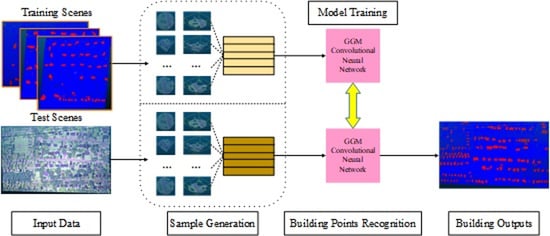
After data preprocessing, we obtain the available multi-spectral LiDAR data. As a supervised method, we have to manually label each of the selected training and test areas before we feed them into the framework. As shown in
Figure 3, our proposed deep learning-based building extraction framework consists of two main stages. First, we feed the labeled training scenes into the GGM convolutional neural networks. Then, we use the trained model to recognize the building points from the input test scenes. Remarkably, the framework requires only point cloud data as the input and directly outputs the labels of each point in the test scenes. There are no limitations about the number of training and test scenes and the size of each input scene. The framework requires no assumptions of the shape and size of the buildings. Furthermore, the model used for training and test is replaceable. That is, any networks, only if they can output the required data form, can be applied in this framework.
During the sample generation stage, the training and test scenes are split into individual samples with a fixed size. Thus, the sampled data can be directly fed into the neural networks, and the input scenes are completely covered by the sampled data at the same time. The details are illustrated in
Section 4.2.
For the building points recognition task, we designed a convolution operator, called GGM convolution, which learns local geometric features from geometric moments representation of a local point set. Then, a hierarchical architecture equipped with the GGM convolution contributes to our model, called GGM convolutional neural networks. The related details are illustrated in
Section 4.3.
4.2. Sample Generation
To keep the scene integrity and ensure every point in the original scene being labeled, inspired by RandLA-Net [
33], we propose a farthest point sampling–k nearest neighbors (FPS-KNN) sample generation method to generate the training and test samples for neural networks. The samples generated by the FPS-KNN both satisfy the input data form requirement of standard convolutional neural networks and obtain the full coverage of the scene.
Figure 4 shows the data processing workflow with the FPS-KNN method. The details of the FPS-KNN sample generation method are carried out as follows:
Step 1: For a given scene, we duplicate an identical point set as the evaluation point set. We randomly choose one point in the evaluation point set as the seed point and search its k nearest neighbors in the original point set. The value of k is set depending on the sample size. For example, if each sample contains 4096 points, then the value of k is configured as 4096.
Step 2: We calculate the distance from the rest points in the evaluation point set to the seed point and select the most distant point as the next seed point. The seed point and its k nearest neighboring points are saved as one sample and removed from the evaluation point set.
Step 3: We iteratively search the farthest point as the seed point in the evaluation point set, search its k nearest neighbors in the original point set, and remove the sampled points from the evaluation point set, until the evaluation point set is empty.
Thus, we obtain numerous samples with the fixed number of points from the given scene, which can be directly fed into a standard convolutional neural network. At the same time, we can ensure that every point in the scene is contained in some samples, which means the full coverage of the scene. We also notice that some samples are inevitably overlapped. For the points within the overlapped part, we choose the most predicted label as its final predicted label.
In this way, theoretically, for any scene, the generated samples can be directly fed into the neural networks by the proposed FPS-KNN sample generation method to obtain the predicted label for every point in the scene.
4.3. Graph Geometric Moments Convolutional Neural Networks
4.3.1. Geometric Moments
Moments and functions of moments have been widely utilized as pattern features in pattern recognition [
34,
35,
36], edge detection [
37,
38], image segmentation [
39], texture analysis [
40], and other domains of image analysis [
41,
42] and computer vision [
43,
44].
The general two-dimensional
th order moments of a density distribution function
is defined as follows:
where
. The lower order moments (small values of
and
) have well defined geometric interpretations. For example,
is the area of the region,
and
give the
and
coordinates of the centroid of the region, respectively [
38]. Similarly, the three-dimensional geometric moments of
th order of a 3D object is defined as follows [
39]:
where
. The discrete implementation of the moments of a 3D homogeneous object could be defined as follows [
38]:
where
is a 3D region. For the 10 low order 3D moments (order up to 2), we have:
For a raw point cloud, we define its geometric moments representation referring to [
45] as follows:
where
and
are the first and second order geometric moments of a point cloud, respectively. Usually, parameters fitting ability is one of the most fundamental and powerful abilities of neural networks. The different order of geometric moments representation of point clouds could be seen as the spatial distribution function with the different variables and orders. Thus, it can upgrade the neural networks to learn more precise features by feeding the geometric moments representation of point clouds.
Besides, the moment-based methods have advantageous qualities like translation and rotation invariance, both of which are important properties for feature descriptors. Translation invariance is obtained by using the central moments for which the origin is at the centroid of the density function [
40]. For 3D objects, the translation invariance is obtained by using the central moments
defined in the same way as for 2D objects [
34]. The central moments
is defined as follows:
where
is the centroid of the object, which can be obtained from the first order moments,
The higher order moments represent more detailed shape characteristics [
40], which means more comprehensive geometric features in deep learning. Mo-Net [
45] first utilizes the second order geometric moments representation of point clouds as the input features. Compared with PointNet [
46], which only considers the first order geometric moments, Mo-Net validates the function of higher order geometric moments. Inspired by that, we design our network to learn features from the geometric moments representation of point clouds.
4.3.2. Graph Generation
Since the graph neural networks (GNNs) proposed by [
47], it has been widely used in learning on unstructured data. GNNs apply neural networks for walks on the graph structure, propagating node representations until a fixed point is reached. The resulting node representations are then used as features in classification and regression problems [
48]. To apply the graph neural network to the point cloud, first, we need to convert it to a directed graph.
A graph is a pair with denoting the set of vertices and representing the set of edges. As the consideration of computational complexity, most of the networks would rather construct a k-nearest neighbors (KNN) than a fully connected edges for the whole point cloud.
As shown in
Figure 5, we utilize the k-nearest neighbors of each point to construct a local directed graph. In this local directed graph, point
is a central node, and
are the edges between the central node and its k-nearest neighbors, which are calculated as follows:
where
are the neighbors of the central point
.
4.3.3. GGM Convolution
In this section, first, we detailed introduce the design of the GGM convolution, which acts as the core module of our model, and then analyze the reason why we design in this way.
Generally, the core module could be seen as an encoder with the given input and output dimension. Meanwhile, to fit various network architectures, the core module should be designed with sufficient universality and pluggability, such as the EdgeConv in DGCNN and relation-shape convolution in RS-CNN. Inspired by the previous core modules, we design the GGM convolution by using the geometric moments representation of point clouds,
Figure 6 shows the details of the GGM convolution.
Given a
-dimensional point cloud with
points, denoted by
. For the initial input,
= 3, which indicates the spectral values of three channels. In a hierarchical neural network, the subsequent layer operates on the output of the previous layer, so more generally the dimension
represents the feature dimension of a given layer [
49], which indicates as the point features in
Figure 6.
As show in
Figure 6, the point features are combined with its 3D coordinates as the input to the GGM Convolution, and the GGM Convolution contains two main branches. The bottom branch indicates the input point features directly fed into a multi-layer perceptron (MLP), which is a skip connection like residual block. The other branch is designed to extract the local features of each point. Firstly, we construct a local directed graph by searching its k-nearest neighbors and calculate the first and second order geometric moments representations of the point and its local directed edges, respectively. Then, they were separately fed into two independent MLPs, and the output of the MLP on the top branch is aggregated by the average-pooling operation. Finally, an addition operation is utilized to fuse all the outputs.
The analysis of local features aggregation strategy: The reason why we use the average-pooling operation instead of the max-pooling operation to aggregate the extracted local features is that we want to obtain the local feature as the compensation of the point feature. The max-pooling operation takes only the max value at each feature channel, which tends to capture the most “special” features and shows less representativeness. To guarantee the extracted compensation feature is sufficiently reliable, the more reasonable local feature should be the average of all local features extracted from the edges.
The analysis of global features aggregation strategy: Although the concatenation and multiplication operations are quite commonly used in related methods. For example, PointNet++ [
50] and DGCNN [
49] fuse features by using concatenation operation, RS-CNN [
51] and GACNet [
52] fuse features by using multiplication operation. Here, we choose the addition operation to fuse features. The main reasons are as follows: (1) the concatenation operation is effective to fuse the multiscale features, and the multiplication operation is commonly used in attention mechanism methods. However, we are fusing the features extracted from higher order geometric moments of original coordinates, which contain different forms of underlying geometric information. Thus, we cannot use the concatenation or multiplication operations roughly here. (2) Essentially, the feature space in deep learning is a kind of probability space, the convolution could be viewed as the filter. The value in different channel of the output feature shows the probability that passes the filter with specific parameters. The addition operation could highlight the befitting filters and restrain the improper filters, which effectively refine the point feature.
4.3.4. Network Architecture
Figure 7 shows the detailed architecture of the GGM Convolutional Neural Networks. The network follows the widely used hierarchical structure. After sample generation, the point clouds of each test area are split into many batches, and each batch contains 4096 points. Through the GGM Convolutional Neural Networks, the input points, which contains spatial coordinates and spectral values of three channels, are labeled with their predicted labels, e.g., 1 indicates the building point and 0 indicates the background point. The details of the GGM Convolutional Neural Networks are illustrated as follows:
Hierarchical structure: Our hierarchical structure is referenced from PointNet++. The hierarchical structure is composed of a number of set abstraction levels. The set abstraction level is made of the following two key layers: the sampling layer and the GGM convolution layer. The sampling layer selects a set of points from the input points via the Farthest Point Sampling (FPS) algorithm, which defines the centroids of local regions. The GGM convolution layer is illustrated in
Section 4.3.3, which combines local feature extraction and grouping function. A set abstraction level takes an
matrix as input that is from
points with
-dimensional coordinates and
-dimensional point feature. It outputs an
matrix of
subsampled points with
-dimensional coordinates and new
-dimensional feature vectors summarizing local features.
Farthest point sampling (FPS): In the sampling layer, we utilize iterative farthest point sampling (FPS) to choose a subset of points. Given the input points , firstly, the FPS randomly picks one point as the seed point, then, calculates the distance from the input points to the seed point and selects the most distant point as the next seed point. The selected points will be removed from the input points. Finally, all the selected seed points constitute the subset of input points with a specified size. In this way, the selected subset of input points could have good coverage of the entire input points.
Multi-scale grouping (MSG): Inspired by PointNet++, we implement the MSG strategy to make our model more robust. For every set abstraction level, we apply a GGM convolution with three different scales, e.g., we set the k-nearest neighbors of 16, 32, and 48 for the first set abstraction level. Then, the features at different scales are concatenated to form a multi-scale feature. Thus, as shown in
Figure 7, we use 3*D to indicate the number of scales and the dimension of features at different scales, respectively.
Feature propagation (
FP): To predict the labels for all the original points, we need to propagate features from subsampled points to the original points. Here, we choose a hierarchical propagation strategy similar to PointNet++. Firstly, we find one nearest neighboring point for each point, whose point feature set is up-sampled through a nearest-neighbor interpolation. Then, the up-sampled features are concatenated with the intermediate feature produced by set abstraction layers through skip connections, which is indicated by the dotted lines in
Figure 6. Finally, we apply a shared MLP and ReLU layer to the concatenated features to update each point’s feature vector.
Final label prediction: The final label of each point is obtained through two shared MLP with 128 and two output dimensions. After a softmax operation, the max value of the two channels indicates the final predicted label.
6. Discussion
Building extraction is a basic task to the applications of land use survey and population change evaluation. According to the statistics in [
2], 40% building extraction methods utilizes the additional data as the compensation of LiDAR data. Although the LiDAR data have been long-term considered as a promising data source, which contain the precious geometric information of the real world, its potential is still not fully realized by the existing methods. The newly emerged multi-spectral LiDAR data provide rich spectral information without the regular data fusion, which inspired us trying to explore the extraction effects with this new data.
As we mentioned before, those common drawbacks of the traditional building extraction approaches (classical machine learning-based methods) might fail to extract buildings from LiDAR data. We think these problems or drawbacks are basically coming from two stages, feature extraction and feature classification. For early studies, because there is no good feature extractor or encoder, they have to extract features manually, which limits the distinguishability and representability of the extracted features. Apparently, without a “good” feature, there is no “good” extraction result. Moreover, the traditional classifiers, which are based on classical machine learning methods, are suitable for small data sets and low-level features, have difficulty handling the large data volume and high-level features. Additionally, the traditional classifiers need to specify the parameters, the researchers are always beset by which classifier should be used and how to adjust its parameters. With the powerful inference ability of CNNs, the deep-learning-based methods automatically learn the high-level features from low-level features, like original coordinates and spectral values, and also learn the suitable or useful features automatically. Besides, the deep learning-based methods could be used as a classifier naturally, and the parameters contained in the network are adjusted by the optimizer automatically. Compared with the traditional approaches, the deep learning-based methods could effectively solve the main drawbacks without extra assumptions or limitations.
Although the deep-learning-based methods have obvious advantages for building extraction tasks, the existing approaches and frameworks still have room for improvement. Due to the unstructured properties of point clouds, the characteristics of point clouds in sparsity, permutation invariance, and transformation invariance, are the thorny problems for standard convolution implementations [
54]. In previous studies, many researchers transformed the point cloud data into multi-view projected images or voxel grids before feeding them to a standard convolutional neural network. Few researchers separated the whole scene into many cuboid regional subsets, and utilized the down-sampling and up-sampling techniques to meet the data form requirement of the standard convolutional neural networks. However, the number of points in unit area is not fixed and the sampling techniques damage the scene integrity, which cannot ensure that every point in the original scene could be labeled. Unlike the existing deep-learning-based point classification frameworks, whose main purpose is to evaluate the accuracy of the model, the building extraction is a practical task, in which every point in the test scenes needs to be predicted for the future real-world applications. That motivated us to develop a new framework. Fortunately, we eventually address these issues by introducing the FPS-KNN sample generation method into the framework. Obviously, the proposed framework also could be applied to the other similar practical tasks, e.g., land cover classification. The limitations of the proposed framework mainly reflect in two ways: the hardship of manually labeling sample and the requirement of massive training data. However, these are the common drawbacks of deep-learning-based frameworks or methods, and there are still no good solutions so far.
Compared with the other state-of-the-art networks, we introduced the geometric moments into our model to extract the local geometric feature more efficiently. Because the special geometry of the buildings or rooftops, e.g., they are normally composited by a set of planar faces, the geometric moments representation contributes to distinguish the building points from the background points significantly. Although the other general models may achieve higher accuracies on benchmarks, our designated model achieves better performance on building extraction tasks. Through the experiments in
Section 5.4, the accuracies and visualization results demonstrated the effectiveness and efficiency of the proposed framework and methods. It is worth mentioning that the test scenes we used are more complicated than the commonly used urban areas, which dramatically increase the difficulty for building extraction tasks. The point-based evaluation we used has higher resolution, which means the stricter evaluation way, compared with pixel-based and object-based evaluations.
Besides, we specially designed the experiments in
Section 5.3.1. On the one hand, we want to investigate and evaluate the effect of additional spectral information. On the other hand, we want to confirm the universality of our model and framework for its future potential extensions. The results confirm our speculations. This motives us to explore the combination of the other additional information, e.g., normal vectors, in our future work.
Since the large volume of point clouds, the inefficient massive data processing of the existing methods has been the obstruction of practical applications. Compared with the classical machine learning based methods, the deep-learning-based methods show significant improvement in this respect, but still limited. For example, with the limitation of GPU memory, by using our model, we can only set the maximum sample size and batch size as 4096 and 16, respectively. It is far from the requirement of building extraction from large scale scenes. In addition, the experiment we designed in
Section 5.3.2 demonstrated that the larger sample size contributes to the better performance. Thus, how to improve the architecture of our model with larger sample size to handle the large-scale building extraction tasks would be our next work.
7. Conclusions
In this paper, we proposed a novel deep-learning-based framework for building extraction from multi-spectral point cloud data. Meanwhile, a sample generation method, a convolution operator and a convolutional neural network implemented in the framework were proposed. The proposed framework provided a novel architecture for the better application of deep learning methods in this research field. Besides, with the characteristic of good universality, theoretically, the proposed framework could handle any point sets and be implemented in any networks, which could greatly promote the practical applications of the proposed framework. As for the point-based evaluation we used in this paper, obviously, it is more difficult to achieve the same accuracy compared with the traditionally used pixel-based and object-based evaluation. However, it has higher resolution and reflects the direct connection with the real world, which is of greater practical significance. Compared with the other state-of-the-art networks, our method achieved the best comprehensive performance with regard to the four metrics. In addition, the corresponding visualization results showed the strong capacity of our model, especially for the difficult cases such as the buildings surrounded by tall trees and the multi-story buildings with complex structure rooftops, our model still achieved outstanding performance than the others. In future work, we will test the influence of adding the other additional features to our method and try to process the larger area scenes by using our method in our framework.

 ,
, 


