A Multi Sensor Approach to Forest Type Mapping for Advancing Monitoring of Sustainable Development Goals (SDG) in Myanmar

Abstract

Monitoring forests is important for measuring overall success of the 2030 Agenda because forests play an essential role in meeting many Sustainable Development Goals (SDG), especially SDG 15. Our study evaluates the contribution of three satellite data sources (Landsat-8, Sentinel-2 and Sentinel-1) for mapping diverse forest types in Myanmar. This assessment is especially important because Myanmar is currently revising its classification system for forests and it is critical that these new forest types can be accurately mapped and monitored over time using satellite imagery. Our results show that using a combination of Sentinel-1 and Sentinel-2 yields the highest accuracy (89.6% ± 0.16 percentage point(pp)), followed by Sentinel-2 alone (87.97% ± 0.11 pp) and Landsat-8 (82.68% ± 0.13 pp). The higher spatial resolution of Sentinel-2 Blue, Green, Red, Narrow Near Infrared and Short Wave Infrared bands enhances accuracy by 4.83% compared to Landsat-8. The addition of the Sentinel-2 Near Infrared and three Vegetation Red Edge bands further improve accuracy by 0.46% compared to using only Sentinel-2 Blue, Green, Red, Narrow Near Infrared and Short Wave Infrared bands. Adding the radar information from Sentinel-1 further increases the accuracy by 1.63%. We were able to map the two major forest types, Upper Moist and Upper Dry Mixed Deciduous Forest, which comprise 90% of our study area. Accuracies for these forest types ranged from 77 to 96% depending on the sensors used, demonstrating the feasibility of using satellite data to map forest categories from a newly revised classification system. Our results advance the ongoing development of the National Forest Monitoring System (NFMS) by the Myanmar Forest Department and United Nations-Food and Agriculture Organization (UN-FAO) and facilitates future monitoring of progress towards the SDGs.

1. Introduction

Forests play an essential role in addressing the Sustainable Development Goals (SDG) set by the United Nations in the 2030 Agenda, by providing goods and services necessary to meet the SDGs [1,2]. Specifically, SDG 15 (Life on Land) explicitly mentions forests and sustainable forest management in its targets 15.1 and 15.2, respectively. Afforestation and halting deforestation are recognized as key pathways for countries to reach their mitigation targets, because forests can serve as major carbon sinks (SDG 13). Given the significant contribution of forests to the SDGs, monitoring of forests is critical to measuring overall success of the 2030 Agenda.

In the context of SDG 15, accurate information on a country’s forest area, as implied by indicator 15.1.1, is dependent on many factors including definitions of national classifications, data source and methodology [3]. Ensuring high quality data for monitoring and reporting, specifically accurate and up-to-date forest type baseline data, remains a logistic, financial and technical challenge in many countries, including Myanmar [4].

Myanmar lies in the Indo-Burma biodiversity hotspot [5] and has the highest forest cover in mainland Southeast Asia [6]. In 2011, the country started the process of political transition from a military government to a democracy accompanied by the opening of its economy. This led to a surge in foreign investments and resulted in increased deforestation. Myanmar had the third highest rate of deforestation globally between 2010 and 2015 [7]. In response, the Government is strengthening the existing National Forestry Master Plan which aims at demarcating 30% of the country’s area for permanent forest cover and 10% of country’s total area for protected areas [7] and has established ambitious targets for reducing emissions from land use change and forestry under the 2015 Paris Agreement and the Nationally Determined Contributions (NDCs), presently in the process of updating. However, different forest types differ in their conservation value, representation within protected areas and vulnerability to loss and degradation. A primary challenge for the management of Myanmar’s unique forests is the absence of recent and accurate forest type maps. Furthermore, forest type definitions differ by national and international agencies and do not accurately represent the forest types at subnational levels. To address this issue, the Myanmar Forest Department is working with the United Nations-Food and Agriculture Organization (UN-FAO) to harmonize and modernize the forest type classifications under the United Nations Programme on Reducing Emissions from Deforestation and Forest Degradation (UN-REDD Programme) supported enhancement of the National Forest Monitoring System (NFMS). An important consideration while developing the revised forest type classification is the feasibility of using current satellite data sources to map the revised forest types accurately.

Earth observations recorded from various platforms (satellite, airborne or ground based) have been widely used to monitor forests because they allow for collecting information about large spatial areas more efficiently compared to ground surveys only [8,9,10,11,12]. Landsat has been traditionally used for most landscape level land cover mapping applications [13,14,15] including forest mapping [16,17,18,19]. The launch of Sentinels (1-2) provided an unprecedented opportunity to advance forest mapping applications [20,21,22,23,24] because of its improved spatial and spectral resolution [25,26]. Sentinel-2 (A and B) has more spectral bands (13 Sentinel-2 vs. 7 Landsat-8 bands), including three Vegetation Red Edge (VRE) and one Narrow Near Infrared (NNIR) bands. The VRE bands are expected to contribute to improved vegetation mapping [25,26,27,28]. Additionally, the R, G, B and NIR bands at higher spatial resolution (10 m for Sentinel-2 vs. 30 m for Landsat-8) and 10 m C band radar from Sentinel-1 are expected to facilitate better vegetation composition mapping [29,30,31].

Studies evaluating Landsat-8 and Sentinel-2 imagery to map land-cover land-use change [26,32], forests attributes such as forest successional stages [33], canopy cover and leaf area index [27] and other forest variables such as stem volume, stem diameter, tree height and basal area [25], have found Sentinel-2’s performance comparable to or better than Landsat-8 depending on the band combination used in the evaluation process. Classification of land use and land cover in Burkina Faso [19] using all Sentinel-2 bands produced an overall accuracy that is 5% higher than using Landsat-8 bands only, while classification of land use and land cover using Sentinel-2 bands, similar to Landsat-8, improved accuracy by 4%. Sentinel-2 outperformed Landsat-8 in forest variable prediction on account of its Vegetation Red Edge band and better spatial resolution. In their study, [25] found that the average of the absolute value of the relative systematic error was 0.8% for Sentinel-2 and 1.2% for Landsat-8. However, research in boreal forests shows that the performance of Sentinel-2 was comparable or slightly better than Landsat-8 in discrimination of different successional forest stages (kappa = 0.98 vs. 0.9) [25] and estimation of canopy cover (root mean square error = 24% vs. 24.5%) and leaf area index (root mean square error =19.6% vs. 20.2%) [20]. Though studies have been conducted on the synergistic use of Landsat-8, Sentinel-2 and Sentinel-1 on the topics of land cover change, successional stages of tropical forests and forestry related variables, only one study has evaluated the potential of Sentinel-1 and -2 to classify detailed tropical forest types [34].

Random Forest is a popular machine learning algorithm for classifying large multiclass datasets as it effectively handles multi-collinearity and noise in multidimensional, non-parametric datasets, without overfitting. It works well even with datasets that have a large number of predictive variables [35,36]. Random Forest algorithm has been widely used in applications ranging from urban mapping [37,38] to forestry [35], exploiting information from spectral reflectance, texture and spatial metrics [39] derived from remotely-sensed datasets. Other methods of statistical analysis, such as discriminant analysis and logistic regression, have been used successfully to differentiate tillage classes in Nebraska from Landsat-5 TM [15]. A comparison of six base models of supervised classification, which included linear and quadratic discriminant analysis, logistic regression, classification trees, neural networks and support vector machines, found that Random Forest performed best in the prediction of Oak habitat [40]. Hence, we decided to use a Random Forest algorithm for our study. The availability of free moderate resolution satellite imagery and machine learning algorithms in open source cloud computing platforms provides an opportunity to analyze large satellite datasets quickly and with minimum computing infrastructure [41]. These advances now significantly aid broad-scale mapping for forest monitoring and management applications at subnational, national or continental scales.

Past satellite-based forest mapping studies in Myanmar have focused on assessing changes in forest cover at the national level [6,42] and in forest type at regional level [43] using Landsat images, but the utility of Sentinel-1 and -2 has not been investigated for forest type mapping in Myanmar. We used a Random Forest algorithm implemented in Google Earth Engine (GEE), a web-based cloud computing platform for geospatial analysis [41], to classify forest types from freely available, multi-temporal Landsat-8 and Sentinel-1 and -2 images for the year 2018.

The overall goal of this study is to compare the contribution of multi-temporal images from Landsat-8 and Sentinel-1 and -2 for developing forest type maps focusing on a pilot study area, the Bago Region in Myanmar. This pilot area was selected because its landscape is dominated by Mixed Deciduous Forests which is assumed to represent the largest forest type by area (39%) in Myanmar [44]. Henceforth, Mixed Deciduous Forest is abbreviated to MDF in text, tables and figures.

Our objectives are:

(i)

To provide a simple, open-source method to map forest types using satellite data sources that can be easily adopted by other countries.

(ii)

Test the accuracy of mapping the revised forest classes using recent active and passive sensors—Sentinel-1, Sentinel-2 and Landsat-8.

(iii)

Evaluate the contribution of each sensor and its metrics to successfully map the revised forest types.

We hypothesize that:

• The accuracy of the Sentinel-2-based forest type classifications is higher compared to Landsat-8 because of improved spatial resolution of Sentinel-2 Red (R), Green (G), Blue (B), Narrow Near Infrared (NNIR), Short Wave Infrared 1 (SWIR1) and Short Wave Infrared 2 (SWIR2) bands and the presence of additional three Vegetation Red Edge (VRE) bands and one Near Infrared (NIR) band in Sentinel-2.
• The accuracy of the combined Sentinel-1 and -2 based forest type classification is higher than the Sentinel-2 based forest type classification because the radar data adds more information on vegetation structure and moisture.

2. Methods

2.1. Study Area

The Bago Region is in the southern part of Central Myanmar between 46°45′N and 19°20′N and 94°35′E and 97°10′E (Figure 1). The Bago Yoma mountain range (also known as Pegu Yoma or Pegu Range), runs in a north-south direction and influences the vegetation patterns in the landscape. The elevation ranges from 0 m to 1909 m with mean elevation of 146 m according to the analysis of elevation data from the Shuttle Radar Topographic Mission (SRTM) [45]. According to Geographic Information System (GIS) data shared by the Myanmar Forest Department, there are six major types of forests in Bago, including Bamboo, Indaing Forests, Lower MDF, Upper Dry MDF, Upper Moist MDF, and Swamps. Teak (Tectona grandis) is a commonly occurring species in the MDFs in this region and is commercially logged for its high-quality wood. Extensive logging of teak has resulted in degradation and soil erosion [46]. The Indaing Forests are Deciduous Dipterocarps forests, dominated mainly by Dipterocarpus tuberculatus.

2.2. Data Sources and Processing

2.2.1. Earth Observation Datasets and Processing

We used GEE [41] to select, process and classify dry season images (November 2017–April 2018) from Sentinel-1, Sentinel-2 and Landsat-8. Thus, our forest type map reflects the spatial distribution of different forests in 2018.

(a)

Landsat-8 and Sentinel-2 processing

To select images for analysis, we applied the image quality filter for all Landsat-8 images [47] and a cloud filter (< 50% cloud cover) to all Landsat-8 and Sentinel-2 ‘Top Of Atmosphere (TOA)’ reflectance products. TOA reflectance products are corrected for differences in sun elevation and sun-earth distance to account for spectral variability resulting from differences in acquisition date and time [48]. The image quality of the TOA reflectance products can be further improved by applying atmospheric corrections to yield Surface Reflectance products [49]. However, Surface Reflectance products for Sentinel-2 that cover our study area were not available for the year 2017 in GEE. Hence, to ensure that all our analyses can be transferrable via the GEE cloud computing facility and to maintain consistency between contrasting remote sensing models, we used TOA data products for both Landsat-8 and Sentinel-2. This is a common approach and has been widely implemented in land cover change products [50,51,52]. Cloud masks were applied to all Landsat-8 and Sentinel-2 TOA images based on information available in the Quality Assessment (QA) bands.

All the Landsat-8 bands used in our study have 30 m resolution. Sentinel-2 has four 10 m bands (R, B, G and NIR) and six 20 m bands (VRE1, VRE2, VRE3, NNIR, SWIR1, SWIR2). All the 10 m Sentinel-2 bands were resampled on-the-fly to 20 m using nearest neighbor in GEE to match the coarser resolution data (see https://developers.google.com/earth-engine/scale for on-the-fly resampling).

• (b) Sentinel-1 processing

We used Sentinel-1 Ground Range Detected (GRD) images available in GEE. These images were already calibrated and orthorectified using Sentinel-1 toolbox and have 10 m spatial resolution. For this analysis we chose images collected in Interferometric Wide (IW) swath mode. IW swath mode is the main acquisition mode over land for Sentinel-1. The IW mode collects data in dual polarization. It means that the microwave sensor transmits either horizontally polarized (H) or vertically polarized (V) waves. Depending on the transmission polarization, the received backscatter wave may be of one of the four types: HH (horizontal transmit and horizontal receive), HV (horizontal transmit and vertical receive), VV (vertical transmit and vertical receive) and VH (vertical transmit and horizontal receive) [53]. Details on data acquisition and processing algorithms for Sentinel-1 may be found in the Sentinel-1 User Guide Introduction (https://sentinel.esa.int/web/sentinel/user-guides/sentinel-1-sar) and Sentinel-1 Technical Guide (https://sentinel.esa.int/web/sentinel/technical-guides/sentinel-1-sar). Previous studies have found Sentinel-1 VV and VH polarizations to be useful in forest mapping applications [21,34]; hence, we used both the VV and VH backscatter in this study. As in the previous analysis, we resampled 10 m bands to 20 m.

• (c) SRTM

To include a topographic variable in our analysis we used 30 m resolution SRTM elevation data available in GEE.

2.2.2. Variables Used in Classification

To study the phenological characteristics of different forest types, we created six cloudless, monthly median composites (November(Nov), December(Dec), January(Jan), February(Feb), March(Mar) and April(Apr)) from the available images for Landsat-8 and Sentinel-2. To achieve this, we stacked images based on month and tile and then computed the monthly median value per pixel. We also calculated 18 texture metrics (

Table 1. List of texture metrics and abbreviations used as variables in supervised forest classification from satellite imagery for the Bago Region of Myanmar based on [54,55].

No.	Name of Texture Metric	Abbreviation
1.	Angular Second Moment	asm
2.	Contrast	contrast
3.	Correlation	corr
4.	Variance	var
5.	Inverse Difference Moment (Homogeneity)	idm
6.	Sum of Average	savg
7.	Sum of Variance	svar
8.	Sum of Entropy	sent
9.	Entropy	ent
10.	Difference of Variances	dvar
11.	Difference of Entropies	dent
12.	Information Measures of Correlation 1	imcorr1
13.	Information Measures of Correlation 2	imcorr2
14.	Maximum Correlation Coefficient	maxcorr
15.	Dissimilarity	diss
16.	Inertia	inertia
17.	Cluster Shade	shade
18.	Cluster Prominence	prom

, [54,55]) for each band and month for each sensor. All texture metrics were derived using a 3 × 3 window. Texture metrics [54,55] have been widely used to improve forest classifications [56,57] in complex landscapes [58] and tropical forests [59]. We also computed band ratios for all band combinations for each sensor. Finally, we include monthly Normalized Difference of all bands for Landsat-8 and Sentinel-2.

2.2.3. Masks

To restrict our analysis to forest pixels, we applied three masks: a tree cover mask based on the percent tree cover threshold, a forest loss mask and Normalized Difference Vegetation Index (NDVI) mask.

(a)

The tree cover mask was created using the Treecover2000 layer from Global Forest Change (GFC) 2018 dataset [17]. The Treecover2000 layer from GFC 2018 dataset provides a continuous percent tree cover value for all land pixels for the year 2000. The pixel values of percent tree cover layer range from 0 to 100%. Depending on the biome, Hansen et al., 2010 recommended using a threshold of 25–30% tree cover to identify woody vegetation taller than 5 m as forest. We decided to adopt the threshold of 25% considering the broad range of variation of forest types in Myanmar ranging from dry forests to evergreen forests. Compared to the 10% threshold used by FAO, the 25% threshold is more conservative but is better suited for global scale applications of mid resolution satellite image [60]. Areas with tree cover less than 25% were excluded from analysis.

(b)

The GFC 2018 dataset also provides estimates of annual forest loss for the years 2001–2018. A forest loss mask was created from the year of forest loss layer of the GFC 2018 dataset to remove all pixels which were forested in 2000 but experienced forest loss between 2000 and 2018.

(c)

Since the GFC 2018 product has a ± 1 year variation in the date of image used, and Bago region has high rate of deforestation [46], an additional NDVI mask was developed from the most recent Sentinel-2 image between November to April to ensure that the sampled pixels have vegetation. The NDVI value was computed as:

NDVI = (NIR − R)/(NIR + R)

(1)

where NIR is Sentinel-2, band 8A (Narrow Near Infrared band), and R is Sentinel-2, band 4 (Red band).

We selected pixels with NDVI values greater than 0.34 to further ensure that the samples have vegetation based on the recommendation available at https://custom-scripts.sentinel-hub.com/custom-scripts/sentinel-2/ndvi/ and preliminary analysis of the value that had the best results classifying forests. A threshold of 0.34 was determined based on visual inspection of the landscape.

2.2.4. Training and Validation Datasets

The Myanmar Forest Department provided digital data from District Forest Inventories (DFI) for Bago Region. This data was collected by Department staff during field survey between 2010 and 2017 and it consists of 3180 georeferenced points with forest type information, spaced at 2 km intervals on a rectangular grid.

We overlaid the 3180 points on forest pixels identified earlier. Only points that overlay on forested pixels were selected for further analysis. For our training, we used randomly selected 984 data points that fell inside our forest mask and that represented six major forest types: Bamboo, Indaing Forests, Lower MDF, Upper Dry MDF, Upper Moist MDF and Swamps. Since the study area is dominated by Upper Dry MDF and Upper Moist MDF, the training data points were proportional to the natural distribution of forest types. Swamp= 2.13% (21 points), Bamboo = 2.24% (22 points), Lower MDF = 11.89% (117 points), Upper Moist MDF = 41.15% (405 points), Upper Dry MDF = 39.33% (387 points) and Indaing Forest = 3.25% (32 points). We buffered each point by 20 m and used the resulting polygon to extract the values from multiband image composite.

The validation dataset was created by combining the remaining points of DFI and additional polygons groundtruthed using high resolution image on Google Earth. Additional validation polygons were created for Bamboo, Indaing, Lower MDF and Swamps that have a low number of points within DFI. Validation data for widespread forest types are randomly selected across the scene. However, because of the small coverage of a few forest types in the region, the validation data of those forest types are strategically searched and located around existing DFI data point. We searched high resolution images in Google Earth for rarer forest types around the sampled DFI points and matched them with characteristic spectral properties to identify validation data for rarer forest types. The process is a two-stage cluster sampling process, which is a valid and practical option when search cost and travel cost are prohibiting and when the extent of the study area is extensive [61]. The proportion of validation samples per classes in the validation data is: Swamp = 0.54% (40 pixels), Bamboo = 0.22% (16 pixels), Lower MDF = 0.50% (37 pixels), Upper Moist MDF = 28.9% (2125 pixels), Upper Dry MDF = 69.55% (5114 pixels) and Indaing Forest = 0.27% (20 pixels). The mixed approach of using existing data were possible and augmenting this data for validation, where needed, resulted in a split of 85% to 15% training to validation, respectively [62].

2.3. Analytical Approach and Flow

Our approach combines the time-series of moderate resolution passive (Sentinel-2, Landsat-8) and active (Sentinel-1) satellite datasets to extract spectral and structural information for each forest type and their response to seasonal variations (Figure 2). To identify the important variables for our classification, we extracted the spectral and structural values for each training polygon across all bands in GEE and exported the resulting training dataset to R [63] and ran a Random Forest classifier. The ‘importance’ function in randomForest package [64] in R was used to identify the important variables. In general, increasing the number of variables increases model accuracy. However, since Random Forest models avoid overfitting, after a certain threshold, adding more variables does not necessarily improve model accuracy. This threshold can be determined by plotting a plot of Mean Decrease in Accuracy vs. the model variables using the ‘importance’ function, run in R. For all our models we determined this threshold using the Mean Decrease in Accuracy vs. the model variables plot to ensure that we choose correct number of variables for the models. A plot of the variables introduced vs. the mean decrease in accuracy revealed a clear threshold, beyond which adding new variables did not improve classification accuracy much. The threshold values for the Landsat-8, Sentinel-2 all bands and Sentinel-1 and -2 models was 6, 5.6 and 12. Based on this threshold, we only employed important variables to run our final classification models in GEE. For example, for the Landsat-8 model, a plot of Mean Decrease in Accuracy vs. the model variables revealed that beyond a threshold of 6, adding more model variables did not improve the accuracy much.

To compare classification performance between sensors and to evaluate the contribution of different bands to the overall accuracy of the classification, we created four classification models (

Table 2. Sensors and band combinations used for each model.

Model.	Variables
Landsat-8 Purpose: Baseline model.	Input bands: Landsat-8 bands (B2, B3, B4, B5, B6, B7)
	Total variables: 145 variables derived from these bands (144 variables per month for 6 months and elevation). Total variables = 144 + 1 = 145. Note: The last variable in each model is ‘elevation.’
	The monthly variables included six spectral bands (B2, B3, B4, B5, B6, B7), 15 simple ratios of the band combinations, 15 Normalized Difference of the band combinations, 18 texture metrics for each of the six bands. Monthly variables = 6 + 15 + 15 + 18*6 = 144.
	Based on variable importance, only 18 variables were selected in the final model. They are: 5 Monthly band composites (Blue_Feb, Blue_Mar, Blue_Nov, Blue_Dec, Green_Mar); 11 Texture of monthly band composites (Blue_savg_Jan, Blue_savg_Feb, Blue_savg_Mar, Blue_savg_Apr, Blue_savg_Nov, Blue_savg_Dec, Green _savg_Feb, Green_savg_Mar, Green _savg_Nov, Red_savg_Mar, Red_savg_Nov); 1 Normalized Difference (SWIR1, Red for Apr) and elevation.
	Map resolution 30 m
Sentinel-2 with Landsat-8 like bands Purpose: Shows how increased resolution (30 m Landsat-8 vs. 20 m Sentinel-2) and characteristic wavelength of Sentinel-2 bands comparable to Landsat-8 improves the forest type classification.	Input bands: Sentinel-2 bands comparable with Landsat-8 bands (B2, B3, B4, B8A, B11 and B12).
	Total variables: 145 variables derived from these bands (144 variables per month for 6 months and elevation). Total variables = 144 + 1 = 145.
	The monthly variables included six spectral bands (B2, B3, B4, B5, B6, B7), 15 simple ratios of the band combinations, 15 Normalized Difference of the band combinations, 18 texture metrics for each of the six bands. Monthly variables = 6 + 15 + 15 + 18*6 = 144.
	The same variables as Landsat-8 model was used.
	Map resolution 20 m.
Sentinel-2-all bands Purpose: Shows the contribution of the 3 VRE and 1 NIR bands to forest type mapping.	Input bands: All Sentinel-2 bands (B2, B3, B4, B5, B6, B7, B8, B8A, B11 and B12).
	Total variables: Retained all bands in Model 2 and added 3 VRE and 1 NNIR bands and variables derived from the 3 VRE and 1 NNIR bands and 3 VRE based indices—CCCI, IRECI and S2REP. The total number of variables generated in Model 3 was 285 (284 variables per month times for 6 months and elevation). Total variables = 284 + 1 = 285.
	The monthly variables included 10 Spectral bands (B2, B3, B4, B5, B6, B7, B8, B8A, B11 and B12), 45 Simple Ratios of the consecutive bands, 45 Normalized Difference of the consecutive bands, 4 Indices (EVI, SAVI, AWEI, WRI), 18 Texture metrics of each of the 10 bands. Monthly variables = 10 + 45 + 45 + 4 + 18*10 = 284.
	Based on variable importance, only 17 new variables were added to the existing 18 variables from previous model. The final model had a total of 35 (17 + 18 = 35) variables. The 17 new variables are: 15 Texture of monthly band composites (VRE1_dent_Mar, VRE1_diss_Mar, VRE1_savg, VRE1_savg_Mar, VRE2_savg_Jan, VRE2_savg_Feb, VRE2_savg_Mar, VRE2_savg_Apr, VRE2_savg_Dec, VRE3_savg_Jan, VRE3_savg_Feb, VRE3_savg_Mar, VRE3_savg_Apr, NIR_savg_Feb, NIR_savg_Apr). 1 Normalized Difference (SWIR1, VRE1 for Apr) and elevation. 1 Simple Ratio of bands (Blue, VRE2 for Apr).
	Map resolution 20 m.
Sentinel-1 and -2 Purpose: Shows the contribution of Sentinel-1 radar bands to forest type classification.	Input bands: VV, VH and ratio of VV and VH.
	Total variables: All the variables from Model 3 and added the bands (VV, VH and ratio of VV and VH) from Sentinel-1 (radar) composite and the texture of the 3 Sentinel-1 bands. The total number of variables in Model 4 was 341 (287 per month for 6 months, 18 texture metrics for each of 3 Sentinel-1 bands and elevation). Total variables = 284 + 3 + 3*18 + 1 = 342.
	The monthly variables included 3 bands (VV, VH, ratio of VV and VH) and Texture metrics of each of the 3 bands. Monthly variables = 284 + 3 + 3*18 = 341.
	Based on variable importance, only 6 new variables were added to the existing 35 variables from previous model. The number of variables in the final model was 41 variables (35 + 6 = 41). The 6 new variables are: 6 Texture of monthly band composites (VH_contrast_Dec, VH_dvar_Dec, VV/VH_contrast_Apr, VV/VH_inertia_Apr, VV/VH_savg_Feb, VV_idm_Nov).
	Map resolution 20 m.

). They were: (i) a Landsat-8 Model (ii) a Sentinel-2 with Landsat-8 like bands Model (iii) a Sentinel-2 all bands Model and (iv) a Sentinel-1 and -2 Model. The purpose of this entire study is to show if Sentinel-2 performs better than Landsat-8 (Model 1 and Model 2) and if the new spectral bands of Sentinel-2 and Sentinel-1 (Model 3 and Model 4) increase the accuracy of forest type classification. The purpose of Models 3 and 4 was to show that the new variables generated from using the new spectral bands (VRE1, VRE2, VRE3, NIR) and radar bands (VV, VH) improve the model accuracy by adding more information compared to the existing spectral resolution of Landsat-8 (R,G,B, NIR, SWIR1, SWIR2). Hence, we attribute the improved accuracy of Model 3 and 4 to improved spectral resolution. To keep the models comparable to the baseline model (Model 1), we kept on adding the new variables to existing variables to show how the new variables improve the model accuracy at each step.

During classification in Random Forest, we set the number of trees to 500 and the number of variables/split to the square root of the total number of variables in the model. We also used a ‘seed’ setting equal to 1 for each model rerun so that models could be reproduced reliably. To assess and compare the outputs and performance of our four different models (Landsat-8 Model, Sentinel-2 with Landsat-8 like bands Model, Sentinel-2 all bands Model and Sentinel-1 and -2 Model), we calculated the absolute and percent forest area for each forest type as well as area proportion weighed area estimates, user’s accuracy and overall accuracy with 95% Confidence Intervals [24,65].

3. Results

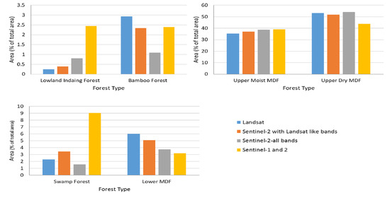
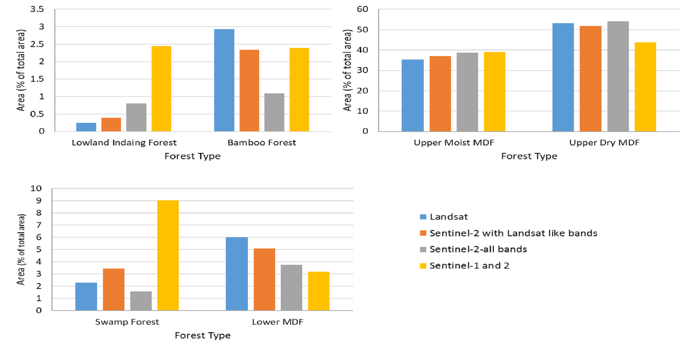
3.1. Areal Estimates

The four (Landsat-8 Model, Sentinel-2 with Landsat-8 like bands Model, Sentinel-2 all bands Model and Sentinel-1 and -2 Model) forest type classifications models produced consistent areal estimates with some minor variation among the forest types (

Table 3. Forest area estimates by different models in Bago Region, Myanmar. The values are in following order, absolute area estimated at pixel level, percentage of total area estimated at pixel level and area estimated with 95% confidence intervals. MDF: Mixed Deciduous Forest.

Model	Swamp [km2/%]	Bamboo [km2/%]	Lower MDF [km2/%]	Upper Moist MDF [km2/%]	Upper Dry MDF [km2/%]	Indaing Forest [km2/%]
Landsat-8	381.17/2.30/ 393.78 ± 0.02	486.46/2.94/ 425.65 ± 0.21	992.59/6.0/ 643.84 ± 0.39	5849.77/35.35/ 7520.16 ± 0.30	8797.72/53.16/ 7522.93 ± 0.54	42.04/0.25/ 43.38 ± 0.04
Sentinel-2 with Landsat-8 like bands	575.04/3.44/ 527.63 ± 112.86	390.04/2.33/ 380.53 ±18.65	854.1/5.10/ 855.26 ±83.05	6182.29/36.95/ 7082.91 ± 150.23	8665.27/51.79/ 7835.85 ± 88.79	65.23/0.39/ 49.78 ± 8.94
Sentinel-2-all bands	261.34/1.56/ 182.94 ± 78.24	182.12/1.09/ 155.47 ± 19.95	629.32/3.76/ 532.44 ± 66.82	6485.4/38.76/ 7492.20 ± 121.04	9040.27/54.03/ 8240.89 ± 84.16	133.51/0.80/ 128.02 ± 14.14
Sentinel-1 and -2	1513.86/9.05/ 1608.17 ± 298.55	399.58/2.39/ 389.83 ± 19.10	536.25/3.2/ 544.30 ± 56.66	6551.12/39.15/ 7436.34 ± 304.68	7322.96/43.77/ 6427.99 ± 73.35	408.28/2.44/ 325.41 ± 54.94

). The largest forest type by area is Upper Dry MDF followed by Upper Moist MDF, Lower MDF, Swamp, Bamboo and Indaing Forests. The highest variation in terms of absolute area is observed for the classes Upper Dry MDF (1717.31 km²), Swamp (568.88 km²) and Upper Moist MDF (321.31 km²) (Table 3).

The swamp has the highest variability in the area, ranging from 2.3% (Landsat-8 model) to 9.05% (Sentinel-1 and -2 model) in the order Sentinel-2-all bands < Landsat-8 < Sentinel-2 with Landsat-8 like bands < Sentinel-1 and -2. The Sentinel-1 and -2 model predicts more Swamp area, almost by a factor of 4 (Figure 3), when compared to the Landsat-8 model. The predicted Landsat-8 Swamp area estimate is 1.5 times smaller when compared to the predicted Swamp area by the Sentinel-2 with Landsat-8 like bands model, though they have same input variables derived from comparable bands. However, the area of Swamp predicted by the Landsat-8 model is 1.5 times more than the Sentinel-2 all band model.

3.2. Spatial Agreement of the Forest Types

A comparison of the maps generated by the four models (Landsat-8 Model, Sentinel-2 with Landsat-8 like bands Model, Sentinel-2 all bands Model and Sentinel-1 and -2 Model) show agreement in most areas except in the northeastern slopes of the Bago Yoma, the east side and southwest side of the maps (Figure 4). All models indicate the presence of Swamp in the northeastern slope of the Bago Yoma and the east side of the map, but the models disagree in the total extent of this forest type. The Sentinel-2 with Landsat-8 like bands model (Figure 4b) and the Sentinel-1 and -2 model classify Swamp (Figure 4d) as the dominant class. The Landsat-8 model classifies this area as Upper Dry MDF (Figure 4a) while adding the VRE bands in the Sentinel-2 all bands model decreases the number of Swamp pixels (Figure 4c).

In the southwest side of the map, the models disagree on the dominant forest type (Figure 4). The Landsat-8 model classifies this area as a mixture of Lower MDF and Swamp, while the Sentinel-2 with Landsat-8 like bands model (Figure 4a,b) classifies this area as Lower MDF. The Sentinel-2 all bands model and Sentinel-1 and -2 model classify it as dominantly Upper Moist MDF (Figure 4c,d).

3.3. Input Predictors and Model Accuracy

Important predictors in the Landsat-8 model included bands B, G, R and SWIR1 (

Table 4. Important predictors in each model.

Model	Important Predictors
Landsat-8	Blue_Feb, Blue_Mar, Blue_Nov, Blue_Dec, Green_Mar, Blue_savg_Jan, Blue_savg_Feb, Blue_savg_Mar, Blue_savg_Apr, Blue_savg_Nov, Blue_savg_Dec, Green _savg_Feb, Green_savg_Mar, Green _savg_Nov, Red_savg_Mar, Red_savg_Nov, Normalized Difference (SWIR1, Red for Apr) and elevation
Sentinel-2-all bands	VRE1_dent_Mar, VRE1_diss_Mar, VRE1_savg, VRE1_savg_Mar, VRE2_savg_Jan, VRE2_savg_Feb, VRE2_savg_Mar, VRE2_savg_Apr, VRE2_savg_Dec, VRE3_savg_Jan, VRE3_savg_Feb, VRE3_savg_Mar, VRE3_savg_Apr, NIR_savg_Feb, NIR_savg_Apr Normalized Difference (SWIR1, VRE1 for Apr) Simple Ratio of bands (Blue, VRE2 for Apr)
Sentinel-1 and -2	VH_contrast_5, VH_dvar_5, VV/VH_contrast_3, VV/VH_inertia_3, VV/VH_savg_1, VV_idm_4

). The Landsat-8 model had the lowest accuracy of all the models (

Table 5. Accuracy of each model in separating forest types in the Bago Yoma of Myanmar.

Model	Accuracy
Landsat-8	82.68% ± 0.13 pp
Sentinel-2 with Landsat-8 like bands	87.51% ± 0.12 pp
Sentinel-2 all bands	87.97% ± 0.11 pp
Sentinel-1 and -2	89.6% ± 0.16 pp

). The Sentinel-2 with Landsat-8 like bands model had the same input variables as the Landsat-8 model; however, it showed improved accuracy of 4.83%. More than 50% of the important variables in Sentinel-2 all band model were derived from the VRE bands and the Sentinel-2 NIR band (Table 4). The addition of the VRE derived metrics improved the accuracy of the Sentinel-2 all band classification by 0.46% compared to the Sentinel-2 with Landsat-8 like bands model. Overall, the Sentinel-2 all bands model had an accuracy of 87.97% ± 0.11 pp, an improvement of 5.3% from the Landsat-8 model.

The savg texture variable appeared most often on the list of important variables (Table 4) in our classification models.

Adding monthly composites and textures of VV, VH and the VV/VH bands (Table 5) in the Sentinel-1 and -2 model increased the accuracy by 1.63% and 6.92% compared to the Sentinel-2 all bands model and Landsat 8 model, respectively (Table 5).

The user’s accuracy for most common and most widely distributed forest types Upper Moist MDF and Upper Dry MDF, together comprising 90% of our study area, varying from 77 to 96% depending on the data source (

Table 6. User’s accuracy for each forest type in each model in separating forest types in the Bago Yoma of Myanmar.

	Model
Forest Type	Landsat-8	Sentinel-2 with Landsat-8 Like Bands	Sentinel-2 -All Bands	Sentinel-1 and -2
Swamp	100.00	90.00	70.00	90.00
Bamboo	87.50	97.56	85.37	97.56
Lower MDF *	64.86	74.42	65.12	86.05
Upper Moist MDF *	93.65	92.89	93.91	96.17
Upper Dry MDF *	76.54	84.43	85.85	84.18
Indaing Forest	50.00	76.32	89.47	76.92

* MDF is an abbreviation of Mixed Deciduous Forest.

).

4. Discussion

In this study we mapped the different forest types in the Bago Region, using satellite data and a revised forest classification provided by the Myanmar Forest Department. According to our maps, the Upper Dry MDF is the largest forest type by area, with its extent ranging between 7322.96 and 9040.27 km², followed by Upper Moist MDF (5849.77– 6551.12 km²). A combination of both the forest types cover approximately 90% of the total forest area in Bago Region. Indaing is the least dominant forest type by area in the region.

Our four models (Landsat-8 Model, Sentinel-2 with Landsat-8 like bands Model, Sentinel-2 all bands Model and Sentinel-1 and -2 Model) showed overall agreement in total area and spatial extent (Table 3 and Figure 4). The disagreement between the four models on the extent of Swamp in the northeastern slopes of the Bago Yoma was investigated in detail due to availability of ground truth data from DFI. The DFI classifies this area as Upper Dry MDF, which is correctly predicted by the Landsat-8 model. Inspection of the area in Google Earth imagery shows it as a low-laying low forest cover region with presence of soil moisture evident from the rivers and streams running into the several lakes in this area. The variation in the model predictions may be explained by the sensitivity of the input variables in each model to soil moisture. The VV band of Sentinel-1 is highly sensitive to soil moisture and the sensitivity decreases with the increase in vegetation cover [66]. Hence, it is no surprise that the Sentinel-1 and -2 model with VV input variable classifies it as Swamp. The Sentinel-2 NIR band (Band 8) in Sentinel-2-all band model includes water absorption wavelengths that were intentionally avoided by the Landsat-8 NIR band design [67] hence, Landsat-8 classifies the same region correctly as Upper Dry MDF, while all the Sentinel-2 models show presence of varying degrees of Swamp pixels. Landsat-8 is known to underestimate the water areas, and often misclassified water with vegetation class in moist conditions [68]. This explains the low presence of Swamp pixels in Landsat-8 model. Despite the Landsat-8 model’s tendency to underestimate Swamps, Sentinel-2 all bands model shows the lowest overall areal estimate of Swamp. A comparison of the maps in Figure 4 shows that some areas classified as Swamp by Landsat-8 and Sentinel-2 Landsat like bands are classified as Upper Moist MDF by Sentinel-2 all bands model. Thus, the confusion of Swamp with Upper Moist MDF in Sentinel-2 all bands model results in underestimation of Swamp.

Accuracy of the forest type classifications varied by sensor and forest type. Absence of overlap between the area weighted overall accuracy and associated 95% confidence intervals show that the differences between the four models are statistically significant (Table 5). Ranked in order of increasing overall accuracy, Landsat-8 (82.68% ± 0.13 pp) < Sentinel-2 bands comparable to Landsat-8 bands (87.51% ± 0.12 pp) < Sentinel-2 all bands (87.97% ± 0.11 pp) < Sentinel-1 and -2 bands (89.6% ± 0.16 pp), proving both our hypotheses to be true. Our first hypothesis holds true as the Landsat-8 based classification showed least accuracy (82.68% ± 0.13 pp) compared to both Sentinel-2 based models (87.51% ± 0.12 pp, 87.97% ± 0.11 pp). Our second hypothesis also holds true as the Sentinel-1 and -2 based classification showed higher accuracy (89.6% ± 0.16 pp) compared to the Sentinel-2 all band model (87.97% ± 0.11 pp). These results can be further explained by considering the role played by important predictors.

Important predictors in Landsat-8 model, included the B, G and SWIR bands. The Blue band is affected by atmosphere, and thus, widely known for its application in coastal and aerosol studies. However, our results are in agreement with previous studies [25,69,70] that found the Blue band to be useful in mapping broadleaf deciduous species. In leaf-off conditions the Blue and Green band of Landsat-8 is more sensitive to stand age in deciduous species [70]. The importance of Blue band can be explained based on the high absorption of blue light (~0.46 µm Landsat-8 Band 2) by chlorophyll b, but not by chlorophylls a, c or d. During the dry season, deciduous plants stop producing chlorophyll in preparation of dry/leaf-off season and, as a consequence, have lower absorption and higher reflectance in blue bands during the dry season when compared to non-deciduous plants. Landsat-8 B band was found to be among the top predictors of tree height and volume in boreal forests [25]. Combination of high-resolution drone imagery B band along with R and G has been shown to separate five deciduous species [69]. The SWIR1 band is sensitive to vegetation moisture [71]. Thus, it is expected that these bands will play an important role in identifying the moist and dry deciduous forests from other forest types.

The improvement of 4.83% accuracy of Sentinel-2 with Landsat-8 like bands model (87.51% ± 0.12 pp) when compared to Landsat-8 model (82.68% ± 0.13 pp) may be attributed to the difference in spatial resolution of Landsat-8 (30 m) and Sentinel-2 (20 m). Sentinel-2, with its higher spatial resolution, results in less mixed class pixels in the training and validation data. Efforts to discriminate grasses grown under different management practices exhibited higher accuracy for simulated Sentinel-2 MSI compared to Landsat-8 OLI (82% vs. 75%) [72]. Additionally, small differences in the wavelengths covered by each band [73] may have affected accuracy.

Comparison of the classification by the Sentinel-2-all bands model to Sentinel-2 with Landsat-8 like bands model highlight the contribution of the VRE and NIR bands to forest type mapping. Adding the different VRE and NIR band metrics increases the accuracy by 0.46% to 87.97% ± 0.11 pp. Similar increases in accuracy have been reported by other studies when using VRE bands in a Random Forest classifier to map land cover [20,21,56].

Addition of the VV and VH bands in Sentinel-1 and -2 model improve the accuracy by 1.63% and show the contribution of the C band radar to forest type mapping over the optical imagery. The radar data complement the optical data and add information on structural components and phenology of the vegetation [74,75]. Both the VV and VH band are sensitive to stem volume [76,77] and were expected to help in separating hardwood forests from Bamboo forest. The Sentinel-1 and -2 model overclassifies the Swamp and Indaing Forests in the landscape. This might be due to Sentinel-1’s sensitivity to soil moisture [66] and limited ability of VH band to discriminate between forest types [34]. Sentinel-1 has been found to have limited improvements over Sentinel-2 in homogeneous forested landscapes [21]; hence, its limited contribution to forest type mapping in Bago, 90% of which is dominated by MDFs, is not unexpected.

Among the texture metrics, the most frequently occurring metric in the important variable list was savg. “savg” is related to tree volume and basal area [78] and its importance can be explained by the dominant presence of big hardwood deciduous trees in the MDFs of Bago Yoma region.

Overall, our analysis shows that a higher resolution, multi-sensor approach using Sentinel-1 and -2 achieves better overall accuracy in mapping forest types in Bago compared to using medium resolution Landsat-8. All our Sentinel-2 based models performed better than Landsat-8 models on account of higher resolution (20 m Sentinel-2 vs. 30 m Landsat-8), added spectral bands (three VRE and one NIR in Sentinel-2) and radar (Sentinel-1) bands. Though the accuracy of the Sentinel based classifications is higher than Landsat-8, Sentinel-2 lacks the temporal legacy of Landsat. Landsat has provided satellite imagery for land cover analysis since 1972, while Sentinel-2 was launched in 2015. The Harmonized Landsat Sentinel-2 (HLS) dataset [79] combines Landsat and Sentinel-2 images to provide dense time series images, which provide improved information on vegetation phenology. The use of HLS datasets may be explored in future studies for forest type mapping. The HLS dataset is corrected for registration errors between Landsat-8 and Sentinel-2. In our study, we used Landsat-8 and Sentinel-2 images separately in the models and did not combine them into a harmonized time-series; thus, we did not co-register the Landsat-8 and Sentinel-2 images. Future studies may also consider using Sentinel-2 Surface Reflectance products, when it is available on GEE.

Our forest type map provides a transparent, unbiased and robust estimate of the distribution of different forest types in Bago Region. Identifying forest type distribution would enable the decision makers to have accurate inventory information on the unique forest resources. Forests play an important role in Myanmar’s economy by providing direct and indirect benefits to many important sectors, such as forestry and agriculture. The combined value of the services that forests provide to the Myanmar economy has been estimated at US$ 7.3 billion each year [80]. Different forest types provide different types of values, goods and services and are exposed to different types of threats. For example, hardwood trees found in mature MDFs are valuable to Myanmar’s economy. However, degradation of the MDFs due to overexploitation of the hardwood species it supports, is a serious environmental issue that needs to be addressed [46]. A distribution map of the MDF forest type is necessary to manage the remaining MDFs sustainably. Similarly, knowing distribution of the bamboo forest type would enable decision makers to formulate poverty alleviation policies, as bamboo and rattan are widely used as building material by people in rural areas. One-fourth of the country’s total population falls under poverty and 85% of the total poor live in rural areas [81] close to forests, and protected areas depend on these resources for survival [82]. The Indaing forests in Central Dry Zone also face intensive anthropogenic pressure for conversion to agriculture [83]. Identification of the current distribution of the threatened Indaing forests from our maps can help the Government to develop policies for forest conservation. Sustainable forest management is, therefore, crucial for Myanmar to achieve the SDGs.

The recent socio-political reform provided the new Government an opportunity to draft new regulations to aid forest conservation. Forest management is recognized as a priority activity, implemented through three main policy and institutional arrangements—National Forestry Master Plan, National Biodiversity Strategies and Action Plan (NBSAP), the REDD+ readiness roadmap, the National REDD+ Strategy and Action Plan and the recently updated NDC for the land use change and forestry sector. In August 2018, the Government of Myanmar adopted the Myanmar Sustainable Development Plan (MSDP), which provides a blueprint of how Myanmar as a nation seeks to achieve sustainable development and contribute to the global SDGs. The MSDP is further divided into three pillars and five goals. Goal 5 addresses the role of forests in achieving sustainability. The absence of a recent forest type map of Myanmar makes it difficult for the Government to manage forest sustainability, and our study fills the gap by demonstrating a forest type mapping methodology for Myanmar that can be scaled to nationwide application. Our study contributes to the Government’s efforts by addressing forest monitoring at a subnational level as most of the interventions contributing to these objectives operate at a local level. The forest type map developed provides a quantifiable baseline against which future changes in forest extent can be evaluated. Information on forest type distribution and quantification of changes in extent of different forest types are important for detailed assessment of carbon storage and international climate reporting requirements. Quantifying change in land cover and identifying the drivers of change also advance our understanding of land cover science.

5. Conclusions

This study demonstrates the utility of recent optical (Landsat-8, Sentinel-2) and radar (Sentinel-1) satellite data to map forest types in Myanmar using a revised forest type classification. Our analysis shows that using Sentinel-2 alone or a combination of Sentinel-1 and Sentinel-2 imagery greatly improves map accuracy (88–90%) compared to only using Landsat-8 (82.68% ± 0.13 pp) imagery. The higher spatial resolution and the characteristic wavelengths of Sentinel-2 improve the accuracy by 4.83% compared to Landsat-8. Addition of the VRE and NIR bands from Sentinel-2 and VV and VH bands from Sentinel-1 further increase the map accuracy by 0.46% and 1.63%, respectively. We were able to map the two major forest types, Upper Moist and Upper Dry MDF, which comprise 90% of our study area, with an accuracy ranging from 77 to 96% for the different sensor specific models, showing the feasibility of using recent satellite data to map the revised forest classifications.

Our approach used freely-available satellite data from the National Aeronautics and Space Administration (NASA) [84,85,86] and the European Space Agency (ESA) [87,88] and all the computation was done using free statistical software R and cloud computing environment of GEE [41], which makes our approach easily transferable across regions. This is especially useful for countries such as Myanmar, which lack recent accurate forest type map and have limited financial and technical resources to meet their international reporting obligations. Our efforts are expected to contribute to the ongoing National Forest Management System (NFMS) conducted by the Myanmar Forest Department and UN-FAO, and contribute to several SDGs, specifically SDG 15, target 15.1.

References

1. Gregersen, H.; El Lakany, H.; Blaser, J. Forests for sustainable development: A process approach to forest sector contributions to the UN 2030 Agenda for Sustainable Development. Int. For. Rev. 2017, 19, 10–23. [Google Scholar] [CrossRef]
2. Seymour, F.; Busch, J. Why forests? Why Now?: The Science, Economics, and Politics of Tropical Forests and Climate Change; Brookings Institution Press: Washington, DC, USA, 2016. [Google Scholar]
3. FAO. Keeping an Eye on SDG 15; FAO: Rome, Italy, 2017; Volume 16. [Google Scholar]
4. Htun, K. Myanmar Forestry Outlook Study; Asia-Pacific Forestry Sector Outlook Study II Working Paper Series; FAO: Rome, Italy, 2009. [Google Scholar]
5. Myers, N.; Mittermeier, R.A.; Mittermeier, C.G.; Da Fonseca, G.A.; Kent, J. Biodiversity hotspots for conservation priorities. Nature 2000, 403, 853–858. [Google Scholar] [CrossRef] [PubMed]
6. Bhagwat, T.; Hess, A.; Horning, N.; Khaing, T.; Thein, Z.M.; Aung, K.M.; Aung, K.H.; Phyo, P.; Tun, Y.L.; Oo, A.H. Losing a jewel—Rapid declines in Myanmar’s intact forests from 2002-2014. PLoS ONE 2017, 12, e0176364. [Google Scholar] [CrossRef] [PubMed] [Green Version]
7. FAO. Global Forest Resources Assessment 2015: How are the World’s Forests Changing? Food and Agriculture Organization of the United Nations: Rome, Italy, 2015. [Google Scholar]
8. Foody, G.M. Remote sensing of tropical forest environments: Towards the monitoring of environmental resources for sustainable development. Int. J. Remote Sens. 2003, 24, 4035–4046. [Google Scholar] [CrossRef]
9. Franklin, S.E. Remote Sensing for Sustainable Forest Management; CRC Press: Boca Raton, FL, USA, 2001. [Google Scholar]
10. Goetz, S.; Dubayah, R. Advances in remote sensing technology and implications for measuring and monitoring forest carbon stocks and change. Carbon Manag. 2011, 2, 231–244. [Google Scholar] [CrossRef]
11. Wulder, M. Optical remote-sensing techniques for the assessment of forest inventory and biophysical parameters. Prog. Phys. Geogr. 1998, 22, 449–476. [Google Scholar] [CrossRef]
12. Fuller, D.O. Tropical forest monitoring and remote sensing: A new era of transparency in forest governance? Singap. J. Trop. Geogr. 2006, 27, 15–29. [Google Scholar] [CrossRef]
13. Hansen, M.C.; Loveland, T.R. A review of large area monitoring of land cover change using Landsat data. Remote Sens. Environ. 2012, 122, 66–74. [Google Scholar] [CrossRef]
14. Sexton, J.O.; Urban, D.L.; Donohue, M.J.; Song, C. Long-term land cover dynamics by multi-temporal classification across the Landsat-5 record. Remote Sens. Environ. 2013, 128, 246–258. [Google Scholar] [CrossRef]
15. Sharma, S.; Dhakal, K.; Wagle, P.; Kilic, A. Retrospective tillage differentiation using the Landsat-5 TM archive with discriminant analysis. Agrosyst. Geosci. Environ. 2020, 3, e20000. [Google Scholar] [CrossRef] [Green Version]
16. Cohen, W.B.; Goward, S.N. Landsat’s role in ecological applications of remote sensing. Bioscience 2004, 54, 535–545. [Google Scholar] [CrossRef]
17. Hansen, M.C.; Potapov, P.V.; Moore, R.; Hancher, M.; Turubanova, S.A.; Tyukavina, A.; Thau, D.; Stehman, S.V.; Goetz, S.J.; Loveland, T.R. High-resolution global maps of 21st-century forest cover change. Science 2013, 342, 850–853. [Google Scholar] [CrossRef] [PubMed] [Green Version]
18. Potapov, P.V.; Turubanova, S.A.; Tyukavina, A.; Krylov, A.M.; McCarty, J.L.; Radeloff, V.C.; Hansen, M.C. Eastern Europe’s forest cover dynamics from 1985 to 2012 quantified from the full Landsat archive. Remote Sens. Environ. 2015, 159, 28–43. [Google Scholar] [CrossRef]
19. Townshend, J.R.; Masek, J.G.; Huang, C.; Vermote, E.F.; Gao, F.; Channan, S.; Sexton, J.O.; Feng, M.; Narasimhan, R.; Kim, D. Global characterization and monitoring of forest cover using Landsat data: Opportunities and challenges. Int. J. Digit. Earth 2012, 5, 373–397. [Google Scholar] [CrossRef] [Green Version]
20. Malenovsky, Z.; Rott, H.; Cihlar, J.; Schaepman, M.E.; García-Santos, G.; Fernandes, R.; Berger, M. Sentinels for science: Potential of Sentinel-1,-2, and-3 missions for scientific observations of ocean, cryosphere, and land. Remote Sens. Environ. 2012, 120, 91–101. [Google Scholar] [CrossRef]
21. Heckel, K.; Urban, M.; Schratz, P.; Mahecha, M.D.; Schmullius, C. Predicting Forest Cover in Distinct Ecosystems: The Potential of Multi-Source Sentinel-1 and-2 Data Fusion. Remote Sens. 2020, 12, 302. [Google Scholar] [CrossRef] [Green Version]
22. Phiri, D.; Simwanda, M.; Salekin, S.; R Nyirenda, V.; Murayama, Y.; Ranagalage, M. Sentinel-2 Data for Land Cover/Use Mapping: A Review. Remote Sens. 2020, 12, 2291. [Google Scholar] [CrossRef]
23. Poortinga, A.; Tenneson, K.; Shapiro, A.; Nquyen, Q.; San Aung, K.; Chishtie, F.; Saah, D. Mapping plantations in Myanmar by fusing landsat-8, sentinel-2 and sentinel-1 data along with systematic error quantification. Remote Sens. 2019, 11, 831. [Google Scholar] [CrossRef] [Green Version]
24. Steinhausen, M.J.; Wagner, P.D.; Narasimhan, B.; Waske, B. Combining Sentinel-1 and Sentinel-2 data for improved land use and land cover mapping of monsoon regions. Int. J. Appl. Earth Obs. Geoinf. 2018, 73, 595–604. [Google Scholar] [CrossRef]
25. Astola, H.; Häme, T.; Sirro, L.; Molinier, M.; Kilpi, J. Comparison of Sentinel-2 and Landsat 8 imagery for forest variable prediction in boreal region. Remote Sens. Environ. 2019, 223, 257–273. [Google Scholar] [CrossRef]
26. Forkuor, G.; Dimobe, K.; Serme, I.; Tondoh, J.E. Landsat-8 vs. Sentinel-2: Examining the added value of sentinel-2’s red-edge bands to land-use and land-cover mapping in Burkina Faso. GISci. Remote Sens. 2018, 55, 331–354. [Google Scholar] [CrossRef]
27. Korhonen, L.; Packalen, P.; Rautiainen, M. Comparison of Sentinel-2 and Landsat 8 in the estimation of boreal forest canopy cover and leaf area index. Remote Sens. Environ. 2017, 195, 259–274. [Google Scholar] [CrossRef]
28. Qiu, S.; He, B.; Yin, C.; Liao, Z. Assessments of Sentinel 2 vegetation red-edge spectral bands for improving land cover classification. Proc. Int. Arch. Photogramm. Remote Sens. Spat. Inf. Sci. 2017, 42, 1055–1059. [Google Scholar] [CrossRef] [Green Version]
29. Drusch, M.; Del Bello, U.; Carlier, S.; Colin, O.; Fernandez, V.; Gascon, F.; Hoersch, B.; Isola, C.; Laberinti, P.; Martimort, P. Sentinel-2: ESA’s optical high-resolution mission for GMES operational services. Remote Sens. Environ. 2012, 120, 25–36. [Google Scholar] [CrossRef]
30. Hojas-Gascon, L.; Belward, A.; Eva, H.; Ceccherini, G.; Hagolle, O.; Garcia, J.; Cerutti, P. Potential improvement for forest cover and forest degradation mapping with the forthcoming Sentinel-2 program. Int. Arch. Photogramm. Remote Sens. Spat. Inf. Sci. 2015, 40, 417. [Google Scholar] [CrossRef] [Green Version]
31. Hirschmugl, M.; Sobe, C.; Deutscher, J.; Schardt, M. Combined use of optical and synthetic aperture radar data for REDD+ applications in Malawi. Land 2018, 7, 116. [Google Scholar] [CrossRef] [Green Version]
32. Chaves, E.D.M.; Picoli, C.A.M.; Sanches, D.I. Recent Applications of Landsat 8/OLI and Sentinel-2/MSI for Land Use and Land Cover Mapping: A Systematic Review. Remote Sens. 2020, 12, 3062. [Google Scholar] [CrossRef]
33. Sothe, C.; Almeida, C.M.; de Liesenberg, V.; Schimalski, M.B. Evaluating Sentinel-2 and Landsat-8 data to map sucessional forest stages in a subtropical forest in Southern Brazil. Remote Sens. 2017, 9, 838. [Google Scholar] [CrossRef] [Green Version]
34. Liu, Y.; Gong, W.; Hu, X.; Gong, J. Forest type identification with random forest using Sentinel-1A, Sentinel-2A, multi-temporal Landsat-8 and DEM data. Remote Sens. 2018, 10, 946. [Google Scholar] [CrossRef] [Green Version]
35. Rodriguez-Galiano, V.F.; Ghimire, B.; Rogan, J.; Chica-Olmo, M.; Rigol-Sanchez, J.P. An assessment of the effectiveness of a random forest classifier for land-cover classification. ISPRS J. Photogramm. Remote Sens. 2012, 67, 93–104. [Google Scholar] [CrossRef]
36. Belgiu, M.; Drăguţ, L. Random forest in remote sensing: A review of applications and future directions. ISPRS J. Photogramm. Remote Sens. 2016, 114, 24–31. [Google Scholar] [CrossRef]
37. Jin, Y.; Liu, X.; Chen, Y.; Liang, X. Land-cover mapping using Random Forest classification and incorporating NDVI time-series and texture: A case study of central Shandong. Int. J. Remote Sens. 2018, 39, 8703–8723. [Google Scholar] [CrossRef]
38. Zhang, H.; Zhang, Y.; Lin, H. Urban land cover mapping using random forest combined with optical and SAR data. In Proceedings of the 2012 IEEE International Geoscience and Remote Sensing Symposium, Munich, Germany, 22–27 July 2012; pp. 6809–6812. [Google Scholar]
39. Ruiz Hernandez, I.E.; Shi, W. A Random Forests classification method for urban land-use mapping integrating spatial metrics and texture analysis. Int. J. Remote Sens. 2018, 39, 1175–1198. [Google Scholar] [CrossRef]
40. Pino-Mejías, R.; Cubiles-de-la-Vega, M.D.; Anaya-Romero, M.; Pascual-Acosta, A.; Jordán-López, A.; Bellinfante-Crocci, N. Predicting the potential habitat of oaks with data mining models and the R system. Environ. Model. Softw. 2010, 25, 826–836. [Google Scholar] [CrossRef]
41. Gorelick, N.; Hancher, M.; Dixon, M.; Ilyushchenko, S.; Thau, D.; Moore, R. Google Earth Engine: Planetary-scale geospatial analysis for everyone. Remote Sens. Environ. 2017, 202, 18–27. [Google Scholar] [CrossRef]
42. Leimgruber, P.; Kelly, D.S.; Steininger, M.K.; Brunner, J.; Müller, T.; Songer, M. Forest cover change patterns in Myanmar (Burma) 1990–2000. Environ. Conserv. 2005, 356–364. [Google Scholar] [CrossRef] [Green Version]
43. Connette, G.; Oswald, P.; Songer, M.; Leimgruber, P. Mapping distinct forest types improves overall forest identification based on multi-spectral Landsat imagery for Myanmar’s Tanintharyi Region. Remote Sens. 2016, 8, 882. [Google Scholar] [CrossRef] [Green Version]
44. Tint, K. Community forestry. In Proceedings of the National Workshop on” Strengthening Re-Afforestation Programmes in Myanmar” Resource Paper, Hamawbi, Myanmar, 29 November–1 December 1995; Volume 6, pp. 68–73. [Google Scholar]
45. Farr, T.G.; Rosen, P.A.; Caro, E.; Crippen, R.; Duren, R.; Hensley, S.; Kobrick, M.; Paller, M.; Rodriguez, E.; Roth, L. The shuttle radar topography mission. Rev. Geophys. 2007, 45, RG2004. [Google Scholar] [CrossRef] [Green Version]
46. Mon, M.S.; Mizoue, N.; Htun, N.Z.; Kajisa, T.; Yoshida, S. Factors affecting deforestation and forest degradation in selectively logged production forest: A case study in Myanmar. For. Ecol. Manag. 2012, 267, 190–198. [Google Scholar] [CrossRef]
47. USGS. Landsat 8 (L8) Data Users Handbook. Available online: https://www.usgs.gov/core-science-systems/nli/landsat/landsat-8-data-users-handbook (accessed on 20 September 2020).
48. Chander, G.; Markham, B.L.; Helder, D.L. Summary of current radiometric calibration coefficients for Landsat MSS, TM, ETM+, and EO-1 ALI sensors. Remote Sens. Environ. 2009, 113, 893–903. [Google Scholar] [CrossRef]
49. Vermote, E.; Justice, C.; Claverie, M.; Franch, B. Preliminary analysis of the performance of the Landsat 8/OLI land surface reflectance product. Remote Sens. Environ. 2016, 185, 46–56. [Google Scholar] [CrossRef] [PubMed]
50. Hansen, M.C.; Egorov, A.; Roy, D.P.; Potapov, P.; Ju, J.; Turubanova, S.; Kommareddy, I.; Loveland, T.R. Continuous fields of land cover for the conterminous United States using Landsat data: First results from the Web-Enabled Landsat Data (WELD) project. Remote Sens. Lett. 2011, 2, 279–288. [Google Scholar] [CrossRef]
51. Liu, Q.; Guo, Y.; Liu, G.; Zhao, J. Classification of Landsat 8 OLI image using support vector machine with Tasseled Cap Transformation. In Proceedings of the 2014 10th International Conference on Natural Computation (ICNC), Xiamen, China, 19–21 August 2014; pp. 665–669. [Google Scholar]
52. Mondal, P.; McDermid, S.S.; Qadir, A. A reporting framework for Sustainable Development Goal 15: Multi-scale monitoring of forest degradation using MODIS, Landsat and Sentinel data. Remote Sens. Environ. 2020, 237, 111592. [Google Scholar] [CrossRef]
53. Flores-Anderson, A.I.; Herndon, K.E.; Thapa, R.B.; Cherrington, E. The SAR Handbook: Comprehensive Methodologies for Forest Monitoring and Biomass Estimation; NASA: Washington, DC, USA, 2019.
54. Haralick, R.M.; Shanmugam, K.; Dinstein, I.H. Textural features for image classification. IEEE Trans. Syst. Man Cybern. 1973, 3, 610–621. [Google Scholar] [CrossRef] [Green Version]
55. Conners, R.W.; Trivedi, M.M.; Harlow, C.A. Segmentation of a high-resolution urban scene using texture operators. Comput. Vis. Graph. Image Process. 1984, 25, 273–310. [Google Scholar] [CrossRef]
56. Kayitakire, F.; Hamel, C.; Defourny, P. Retrieving forest structure variables based on image texture analysis and IKONOS-2 imagery. Remote Sens. Environ. 2006, 102, 390–401. [Google Scholar] [CrossRef]
57. Franklin, S.E.; Hall, R.J.; Moskal, L.M.; Maudie, A.J.; Lavigne, M.B. Incorporating texture into classification of forest species composition from airborne multispectral images. Int. J. Remote Sens. 2000, 21, 61–79. [Google Scholar] [CrossRef]
58. Rodriguez-Galiano, V.F.; Chica-Olmo, M.; Abarca-Hernandez, F.; Atkinson, P.M.; Jeganathan, C. Random Forest classification of Mediterranean land cover using multi-seasonal imagery and multi-seasonal texture. Remote Sens. Environ. 2012, 121, 93–107. [Google Scholar] [CrossRef]
59. Simard, M.; Saatchi, S.S.; De Grandi, G. The use of decision tree and multiscale texture for classification of JERS-1 SAR data over tropical forest. IEEE Trans. Geosci. Remote Sens. 2000, 38, 2310–2321. [Google Scholar] [CrossRef] [Green Version]
60. Hansen, M.C.; Stehman, S.V.; Potapov, P.V. Quantification of global gross forest cover loss. Proc. Natl. Acad. Sci. USA 2010, 107, 8650–8655. [Google Scholar] [CrossRef] [Green Version]
61. McGrew, J.C., Jr.; Monroe, C.B. An Introduction to Statistical Problem Solving in Geography; Waveland Press: Long Grove, IL, USA, 2009. [Google Scholar]
62. Sharma, S.; Ochsner, T.E.; Twidwell, D.; Carlson, J.D.; Krueger, E.S.; Engle, D.M.; Fuhlendorf, S.D. Nondestructive estimation of standing crop and fuel moisture content in tallgrass prairie. Rangel. Ecol. Manag. 2018, 71, 356–362. [Google Scholar] [CrossRef]
63. R Core Team, R. A Language and Environment for Statistical Computing [Computer Software Manual]; R Core Team: Vienna, Austria, 2016. [Google Scholar]
64. Liaw, A.; Wiener, M. Classification and regression by randomForest. R News 2002, 2, 18–22. [Google Scholar]
65. Olofsson, P.; Foody, G.M.; Herold, M.; Stehman, S.V.; Woodcock, C.E.; Wulder, M.A. Good practices for estimating area and assessing accuracy of land change. Remote Sens. Environ. 2014, 148, 42–57. [Google Scholar] [CrossRef]
66. Bousbih, S.; Zribi, M.; Lili-Chabaane, Z.; Baghdadi, N.; El Hajj, M.; Gao, Q.; Mougenot, B. Potential of Sentinel-1 radar data for the assessment of soil and cereal cover parameters. Sensors 2017, 17, 2617. [Google Scholar] [CrossRef] [PubMed] [Green Version]
67. Irons, J.R.; Dwyer, J.L.; Barsi, J.A. The next Landsat satellite: The Landsat data continuity mission. Remote Sens. Environ. 2012, 122, 11–21. [Google Scholar] [CrossRef] [Green Version]
68. Labib, S.M.; Harris, A. The potentials of Sentinel-2 and LandSat-8 data in green infrastructure extraction, using object based image analysis (OBIA) method. Eur. J. Remote Sens. 2018, 51, 231–240. [Google Scholar] [CrossRef]
69. Lisein, J.; Michez, A.; Claessens, H.; Lejeune, P. Discrimination of deciduous tree species from time series of unmanned aerial system imagery. PLoS ONE 2015, 10, e0141006. [Google Scholar] [CrossRef]
70. Li, D.; Ju, W.; Fan, W.; Gu, Z. Estimating the age of deciduous forests in northeast China with Enhanced Thematic Mapper Plus data acquired in different phenological seasons. J. Appl. Remote Sens. 2014, 8, 083670. [Google Scholar] [CrossRef] [Green Version]
71. Barsi, J.A.; Lee, K.; Kvaran, G.; Markham, B.L.; Pedelty, J.A. The spectral response of the Landsat-8 operational land imager. Remote Sens. 2014, 6, 10232–10251. [Google Scholar] [CrossRef] [Green Version]
72. Sibanda, M.; Mutanga, O.; Rouget, M. Discriminating rangeland management practices using simulated hyspIRI, landsat 8 OLI, sentinel 2 MSI, and VENμs spectral data. IEEE J. Sel. Top. Appl. Earth Obs. Remote Sens. 2016, 9, 3957–3969. [Google Scholar] [CrossRef]
73. Chastain, R.; Housman, I.; Goldstein, J.; Finco, M.; Tenneson, K. Empirical cross sensor comparison of Sentinel-2A and 2B MSI, Landsat-8 OLI, and Landsat-7 ETM+ top of atmosphere spectral characteristics over the conterminous United States. Remote Sens. Environ. 2019, 221, 274–285. [Google Scholar] [CrossRef]
74. Erinjery, J.J.; Singh, M.; Kent, R. Mapping and assessment of vegetation types in the tropical rainforests of the Western Ghats using multispectral Sentinel-2 and SAR Sentinel-1 satellite imagery. Remote Sens. Environ. 2018, 216, 345–354. [Google Scholar] [CrossRef]
75. Rüetschi, M.; Schaepman, M.E.; Small, D. Using multitemporal sentinel-1 c-band backscatter to monitor phenology and classify deciduous and coniferous forests in northern switzerland. Remote Sens. 2018, 10, 55. [Google Scholar] [CrossRef] [Green Version]
76. Argamosa, R.J.L.; Blanco, A.C.; Baloloy, A.B.; Candido, C.G.; Dumalag, J.B.L.C.; DImapilis, L.L.C.; Paringit, E.C. Modelling above Ground Biomass of Mangrove Forest Using Sentinel-1 Imagery. ISPRS Ann. Photogramm. Remote Sens. Spat. Inf. Sci. 2018, 4, 3. [Google Scholar] [CrossRef] [Green Version]
77. Jena, F.-S.-U. SAR Theory and Applications to Forest Cover and Disturbance Mapping and Forest Biomass Assessment; Friedrich-Schiller-University: Jena, Germany, 2012; Volume 57. [Google Scholar]
78. Niemi, M.T.; Vauhkonen, J. Extracting canopy surface texture from airborne laser scanning data for the supervised and unsupervised prediction of area-based forest characteristics. Remote Sens. 2016, 8, 582. [Google Scholar] [CrossRef] [Green Version]
79. Claverie, M.; Ju, J.; Masek, J.G.; Dungan, J.L.; Vermote, E.F.; Roger, J.-C.; Skakun, S.V.; Justice, C. The Harmonized Landsat and Sentinel-2 surface reflectance data set. Remote Sens. Environ. 2018, 219, 145–161. [Google Scholar] [CrossRef]
80. Emerton, L.; Aung, Y.M. The Economic Value of Forest Ecosystem Services in Myanmar and Options for Sustainable Financing; International Management Group: Yangon, Myanmar, 2013. [Google Scholar]
81. Assessment, I.H.L.C. Integrated Household Living Conditions Survey 2009-10 Myanmar: Poverty Profile; United Nations Development Programme: Yangon, Myanmar, 2011. [Google Scholar]
82. Rao, M.; Rabinowitz, A.; Khaing, S.T. Status review of the protected-area system in Myanmar, with recommendations for conservation planning. Conserv. Biol. 2002, 16, 360–368. [Google Scholar] [CrossRef]
83. Southeastern Asia: Central Myanmar (formerly Burma)|Ecoregions|WWF. Available online: https://www.worldwildlife.org/ecoregions/im0205 (accessed on 14 August 2020).
84. Loveland, T.R.; Dwyer, J.L. Landsat: Building a strong future. Remote Sens. Environ. 2012, 122, 22–29. [Google Scholar] [CrossRef]
85. Woodcock, C.E.; Allen, R.; Anderson, M.; Belward, A.; Bindschadler, R.; Cohen, W.; Gao, F.; Goward, S.N.; Helder, D.; Helmer, E. Free access to Landsat imagery. Science 2008, 320, 1011. [Google Scholar] [CrossRef]
86. Wulder, M.A.; Masek, J.G.; Cohen, W.B.; Loveland, T.R.; Woodcock, C.E. Opening the archive: How free data has enabled the science and monitoring promise of Landsat. Remote Sens. Environ. 2012, 122, 2–10. [Google Scholar] [CrossRef]
87. Showstack, R. Sentinel satellites initiate new era in earth observation. Eos Trans. Am. Geophys. Union 2014, 95, 239–240. [Google Scholar] [CrossRef]
88. International Cooperation|Copernicus. Available online: https://www.copernicus.eu/en/about-copernicus/international-cooperation (accessed on 13 August 2020).
Figure 1. Location of the study area. The Sentinel-2 image in false color composite RGB: 11, 8, 3 band combination shows the distribution of the forests (green) in the study area.
Remotesensing 12 03220 g001
Figure 2. Overview of image processing and classification steps to map forest types from satellite imagery for the Bago Region of Myanmar. TOA: Top Of Atmosphere; GRD: Ground Range Detected; NDVI: Normalized Difference Vegetation Index.
Remotesensing 12 03220 g002
Figure 3. Variation in percent area estimates for different forest types in the Bago Region of Myanmar. We are comparing different sets of spectral and textual variables from a range of satellite sensors. MDF: Mixed Deciduous Forest.
Remotesensing 12 03220 g003
Figure 4. Comparison of the forest type maps for the Bago Region of Myanmar, based on different combinations of satellite data and derived variables. The black, red and yellow boxes show areas of disagreement. (a) Landsat-8 Model, (b) Sentinel-2 with Landsat-8 like bands Model, (c) Sentinel-2 all bands Model, (d) Sentinel-1 and -2 Model.
Remotesensing 12 03220 g004