Tree Species Traits Determine the Success of LiDAR-Based Crown Mapping in a Mixed Temperate Forest

 , , , ,
Abstract
:
1. Introduction
2. Materials and Methods
2.1. Study Site Description
2.2. Remote Sensing Data
2.3. Crown Delineation
2.4. Parameter Tuning and Accuracy Assessment
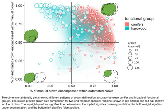
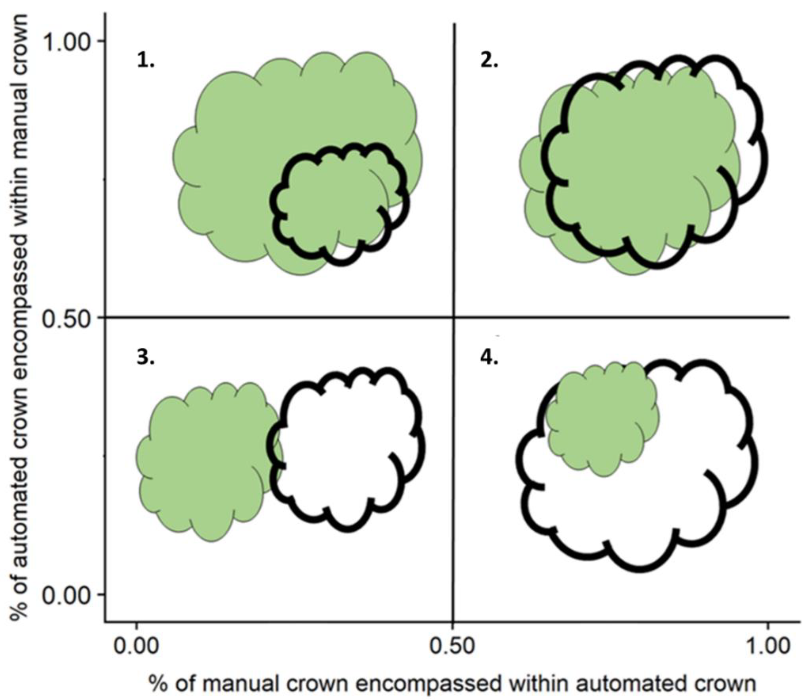
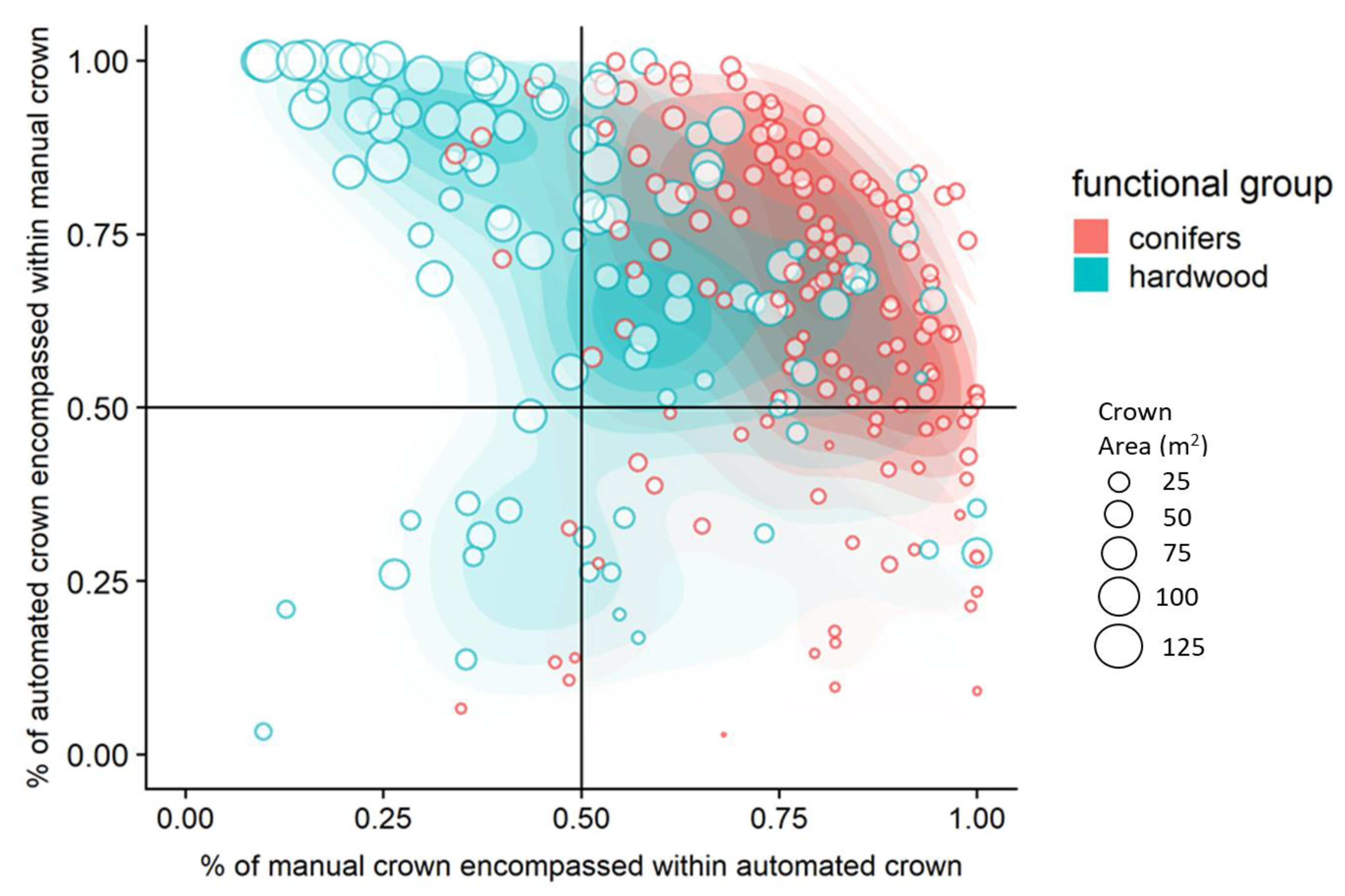
- Over-segmentation: The intersecting area between AITC and MITC is greater than or equal to 50% of the area of only AITC, indicating that the automated crown is smaller than manual crown.
- True Positive: The intersecting area between AITC and MITC is greater than or equal to 50% of the area of both AITC and MITC (as defined above), indicating that the automated crown is well matched to the manual crown.
- Under-segmentation: The intersecting area between AITC and MITC is greater than or equal to 50% of the area of only MITC, indicating that the automated crown is larger than the manual crown.
- False Positive: The intersecting area between AITC and MITC is greater than or equal to 50% of the area of neither AITC and MITC, indicating poor matching of the automated and manual crowns.
2.5. Statistical Analysis
3. Results
3.1. Manual Crown and Plot Characteristics
3.2. Automated Crown Delineation Accuracy
3.2.1. Influence of Parameter Tuning and Differences in Model Accuracies
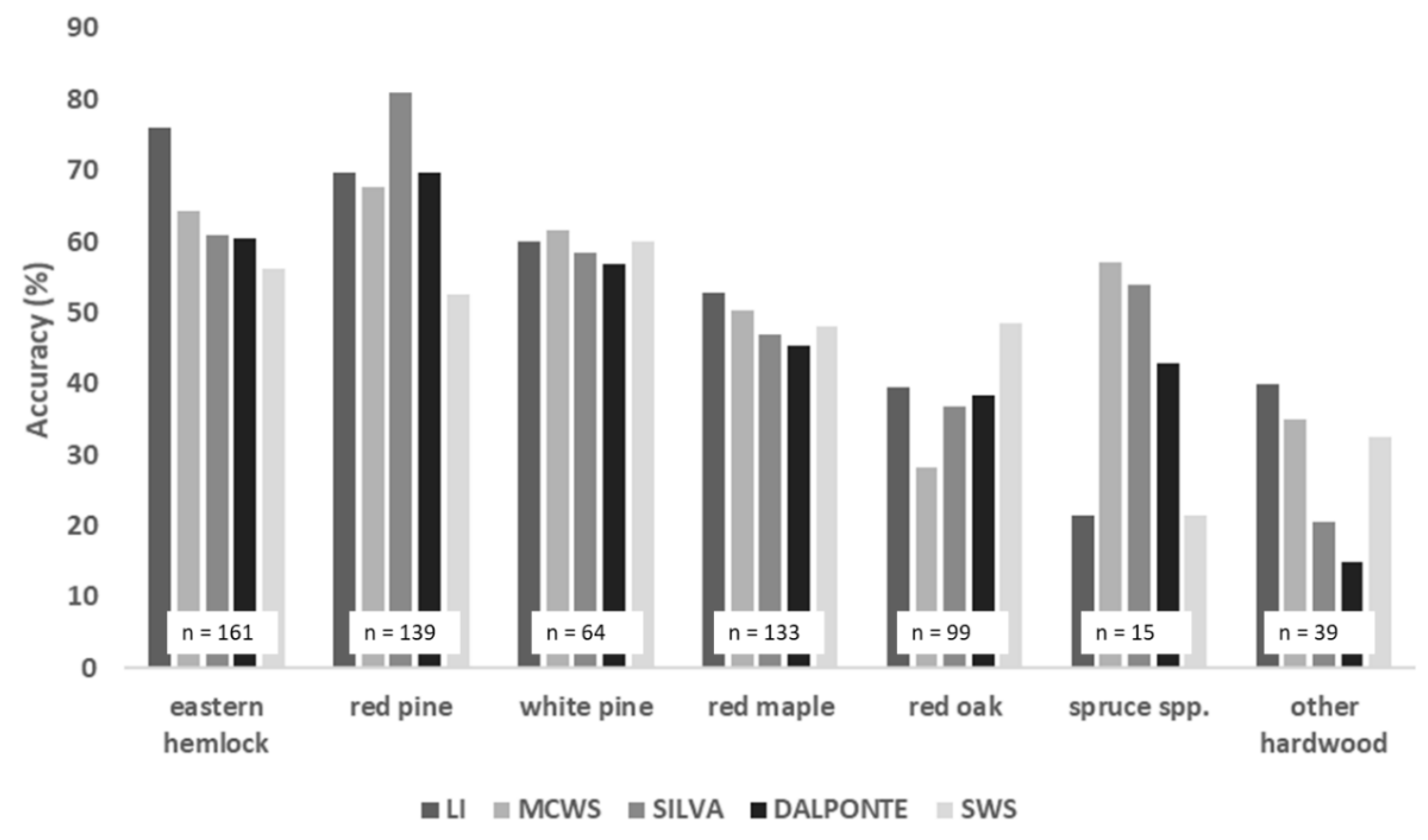
3.2.2. Differences in Accuracy across Species
3.3. Variables Influencing Accurate Automated Crown Delineation
3.3.1. Linear Regressions
3.3.2. Logistic Regressions
4. Discussion
4.1. Differences between Segmentation Methods
4.2. Tree Architecture
4.2.1. Tree Size
4.2.2. Crown Spread
4.2.3. Mechanical Interactions
4.3. Species Evenness
4.4. A Silver Lining: Where Do Automated Crown Delineation Methods Work Well?
4.5. Moving forward
5. Conclusions
Supplementary Materials
Author Contributions
Funding
Acknowledgments
Conflicts of Interest
References
- Shi, Y.; Skidmore, A.K.; Wang, T.; Holzwarth, S.; Heiden, U.; Pinnel, N.; Zhu, X.; Heurich, M. Tree species classification using plant functional traits from LiDAR and hyperspectral data. Int. J. Appl. Earth Obs. Geoinf. 2018, 73, 207–219. [Google Scholar] [CrossRef]
- Zhao, Y.; Zeng, Y.; Zheng, Z.; Dong, W.; Zhao, D.; Wu, B.; Zhao, Q. Forest species diversity mapping using airborne LiDAR and hyperspectral data in a subtropical forest in China. Remote Sens. Environ. 2018, 213, 104–114. [Google Scholar] [CrossRef]
- Coomes, D.A.; Dalponte, M.; Jucker, T.; Asner, G.P.; Banin, L.F.; Burslem, D.F.R.P.; Lewis, S.L.; Nilus, R.; Phillips, O.L.; Phua, M.-H.; et al. Area-based vs tree-centric approaches to mapping forest carbon in Southeast Asian forests from airborne laser scanning data. Remote Sens. Environ. 2017, 194, 77–88. [Google Scholar] [CrossRef] [Green Version]
- Palace, M.; Keller, M.; Asner, G.P.; Hagen, S.; Braswell, B. Amazon forest structure from IKONOS satellite data and the automated characterization of forest canopy properties. Biotropica 2008, 40, 141–150. [Google Scholar] [CrossRef]
- Clark, M.L.; Roberts, D.A.; Clark, D.B. Hyperspectral discrimination of tropical rain forest tree species at leaf to crown scales. Remote Sens. Environ. 2005, 96, 375–398. [Google Scholar] [CrossRef]
- Fang, F.; McNeil, B.E.; Warner, T.A.; Maxwell, A.E. Combining high spatial resolution multi-temporal satellite data with leaf-on LiDAR to enhance tree species discrimination at the crown level. Int. J. Remote Sens. 2018, 39, 9054–9072. [Google Scholar] [CrossRef]
- Zhang, T.; Niinemets, Ü.; Sheffield, J.; Lichstein, J.W. Shifts in tree functional composition amplify the response of forest biomass to climate. Nature 2018, 556, 99–102. [Google Scholar] [CrossRef]
- Seebens, H.; Blackburn, T.M.; Dyer, E.E.; Genovesi, P.; Hulme, P.E.; Jeschke, J.M.; Pagad, S.; Pyšek, P.; Winter, M.; Arianoutsou, M.; et al. No saturation in the accumulation of alien species worldwide. Nat. Commun. 2017, 8, 1–9. [Google Scholar] [CrossRef] [PubMed]
- Houghton, R.A. Land-use change and the carbon cycle. Glob. Chang. Biol. 1995, 1, 275–287. [Google Scholar] [CrossRef]
- Ayrey, E.; Fraver, S.; Kershaw, J.A.; Kenefic, L.S.; Hayes, D.; Weiskittel, A.R.; Roth, B.E. Layer Stacking: A Novel Algorithm for Individual Forest Tree Segmentation from LiDAR Point Clouds. Can. J. Remote Sens. 2017, 43, 16–27. [Google Scholar] [CrossRef]
- Jing, L.; Hu, B.; Noland, T.; Li, J. An individual tree crown delineation method based on multi-scale segmentation of imagery. ISPRS J. Photogramm. Remote Sens. 2012, 70, 88–98. [Google Scholar] [CrossRef]
- Lu, X.; Guo, Q.; Li, W.; Flanagan, J. A bottom-up approach to segment individual deciduous trees using leaf-off lidar point cloud data. ISPRS J. Photogramm. Remote Sens. 2014, 94, 1–12. [Google Scholar] [CrossRef]
- Wan Mohd Jaafar, W.; Woodhouse, I.; Silva, C.; Omar, H.; Abdul Maulud, K.; Hudak, A.; Klauberg, C.; Cardil, A.; Mohan, M. Improving Individual Tree Crown Delineation and Attributes Estimation of Tropical Forests Using Airborne LiDAR Data. Forests 2018, 9, 759. [Google Scholar] [CrossRef] [Green Version]
- Zhen, Z.; Quackenbush, L.J.; Stehman, S.V.; Zhang, L. Agent-based region growing for individual tree crown delineation from airborne laser scanning (ALS) data. Int. J. Remote Sens. 2015, 36, 1965–1993. [Google Scholar] [CrossRef]
- Williams, J.; Schonlieb, C.-B.; Swinfield, T.; Lee, J.; Cai, X.; Qie, L.; Coomes, D.A. 3D Segmentation of Trees Through a Flexible Multiclass Graph Cut Algorithm. IEEE Trans. Geosci. Remote Sens. 2019. [Google Scholar] [CrossRef]
- Dalponte, M.; Reyes, F.; Kandare, K.; Gianelle, D. Delineation of individual tree crowns from ALS and hyperspectral data: A comparison among four methods. Eur. J. Remote Sens. 2015, 48, 365–382. [Google Scholar] [CrossRef] [Green Version]
- Zhen, Z.; Quackenbush, L.J.; Zhang, L. Trends in automatic individual tree crown detection and delineation-evolution of LiDAR data. Remote Sens. 2016, 8, 333. [Google Scholar] [CrossRef] [Green Version]
- Vauhkonen, J.; Ene, L.; Gupta, S.; Heinzel, J.; Holmgren, J.; Pitkänen, J.; Solberg, S.; Wang, Y.; Weinacker, H.; Hauglin, K.M.; et al. Comparative testing of single-tree detection algorithms under different types of forest. Forestry 2012, 85, 27–40. [Google Scholar] [CrossRef] [Green Version]
- Valladares, F.; Niinemets, U. The Architecture of Plant Crowns: From Design Rules to Light Capture and Performance. In Functional Plant Ecology; CRC Press: Boca Raton, FL, USA, 2007; pp. 101–150. [Google Scholar]
- Chave, J.; Coomes, D.; Jansen, S.; Lewis, S.L.; Swenson, N.G.; Zanne, A.E. Towards a worldwide wood economics spectrum. Ecol. Lett. 2009, 12, 351–366. [Google Scholar] [CrossRef]
- Muth, C.C.; Bazzaz, F.A. Tree canopy displacement and neighborhood interactions. Can. J. For. Res. 2003, 33, 1323–1330. [Google Scholar] [CrossRef]
- Pretzsch, H. Canopy space filling and tree crown morphology in mixed-species stands compared with monocultures. For. Ecol. Manag. 2014, 327, 251–264. [Google Scholar] [CrossRef] [Green Version]
- Forrester, D.I.; Benneter, A.; Bouriaud, O.; Bauhus, J. Diversity and competition influence tree allometric relationships—developing functions for mixed-species forests. J. Ecol. 2017, 105, 761–774. [Google Scholar] [CrossRef] [Green Version]
- Fichtner, A.; Härdtle, W.; Li, Y.; Bruelheide, H.; Kunz, M.; von Oheimb, G. From competition to facilitation: How tree species respond to neighbourhood diversity. Ecol. Lett. 2017, 20, 892–900. [Google Scholar] [CrossRef] [PubMed]
- Givnish, T.J. Ecological Constraints on the Evolution of Breeding Systems in Seed Plants: Dioecy and Dispersal in Gymnosperms. Evolution 2002, 34, 959. [Google Scholar] [CrossRef]
- Oliver, C.D.; Stephens, E.P. Reconstruction of a Mixed-Species Forest in Central New England. Ecology 1977, 58, 562–572. [Google Scholar] [CrossRef] [Green Version]
- Brodribb, T.J.; Pittermann, J.; Coomes, D.A. Elegance versus Speed: Examining the Competition between Conifer and Angiosperm Trees. Int. J. Plant. Sci. 2012, 173, 673–694. [Google Scholar] [CrossRef] [Green Version]
- Augusto, L.; Davies, T.J.; Delzon, S.; de Schrijver, A. The enigma of the rise of angiosperms: Can we untie the knot? Ecol. Lett. 2014, 17, 1326–1338. [Google Scholar] [CrossRef]
- Li, W.; Guo, Q.; Jakubowski, M.K.; Kelly, M. A New Method for Segmenting Individual Trees from the Lidar Point Cloud. Photogramm. Eng. Remote Sens. 2012, 78, 75–84. [Google Scholar] [CrossRef] [Green Version]
- Wang, Y.; Hyyppa, J.; Liang, X.; Kaartinen, H.; Yu, X.; Lindberg, E.; Holmgren, J.; Qin, Y.; Mallet, C.; Ferraz, A.; et al. International Benchmarking of the Individual Tree Detection Methods for Modeling 3-D Canopy Structure for Silviculture and Forest Ecology Using Airborne Laser Scanning. IEEE Trans. Geosci. Remote Sens. 2016, 54, 5011–5027. [Google Scholar] [CrossRef] [Green Version]
- Silva, C.A.; Hudak, A.T.; Vierling, L.A.; Loudermilk, E.L.; O’Brien, J.J.; Hiers, J.K.; Jack, S.B.; Gonzalez-Benecke, C.; Lee, H.; Falkowski, M.J.; et al. Imputation of Individual Longleaf Pine (Pinus palustris Mill.) Tree Attributes from Field and LiDAR Data. Can. J. Remote Sens. 2016, 42, 554–573. [Google Scholar] [CrossRef]
- Broadbent, E.N.; Asner, G.P.; Peña-Claros, M.; Palace, M.; Soriano, M. Spatial partitioning of biomass and diversity in a lowland Bolivian forest: Linking field and remote sensing measurements. For. Ecol. Manag. 2008, 255, 2602–2616. [Google Scholar] [CrossRef]
- Anderson-Teixeira, K.J.; Davies, S.J.; Bennett, A.C.; Gonzalez-Akre, E.B.; Muller-Landau, H.C.; Joseph Wright, S.; Abu Salim, K.; Almeyda Zambrano, A.M.; Alonso, A.; Baltzer, J.L.; et al. CTFS-ForestGEO: A worldwide network monitoring forests in an era of global change. Glob. Chang. Biol. 2015, 21, 528–549. [Google Scholar] [CrossRef] [PubMed] [Green Version]
- Orwig, D.; Ellison, A. Harvard Forest CTFS-ForestGEO Mapped Forest Plot since 2014. Environ. Data Initiat. 2015. [Google Scholar] [CrossRef]
- Plotkins, A.B.; O’Keefe, J.; Foster, D.R. Harvard University Forest, Massachusetts, United States of America. In Forest Plans of North America; Siry, J.P., Bettinger, P., Merry, K., Grebner, D.L., Boston, K., Cieszewski, C., Eds.; Academic Press: Waltham, MA, USA, 2015; pp. 69–77. ISBN 9780127999364. [Google Scholar]
- Orwig, D.A.; Boucher, P.; Paynter, I.; Saenz, E.; Li, Z.; Schaaf, C. The potential to characterize ecological data with terrestrial laser scanning in Harvard Forest, MA. Interface Focus 2018, 8, 20170044. [Google Scholar] [CrossRef]
- Sullivan, F.B.; Ducey, M.J.; Orwig, D.A.; Cook, B.; Palace, M.W. Forest Ecology and Management Comparison of lidar- and allometry-derived canopy height models in an eastern deciduous forest. For. Ecol. Manag. 2017, 406, 83–94. [Google Scholar] [CrossRef]
- Cook, B.D.; Corp, L.A.; Nelson, R.F.; Middleton, E.M.; Morton, D.C.; Mccorkel, J.T.; Masek, J.G.; Ranson, K.J.; Ly, V.; Montesano, P.M. NASA Goddard’s LiDAR, Hyperspectral and Thermal (G-LiHT) Airborne Imager. Remote Sens. 2013, 5, 4045–4066. [Google Scholar] [CrossRef] [Green Version]
- Kampe, T.U. NEON: The first continental-scale ecological observatory with airborne remote sensing of vegetation canopy biochemistry and structure. J. Appl. Remote Sens. 2010, 4, 043510. [Google Scholar] [CrossRef]
- Quantum GIS Development Team. Quantum GIS Geographic Information System. Open Source Geospatial Foundation Project. 2018. Available online: http://qgis.osgeo.org (accessed on 10 October 2019).
- R Core Team. R: A Language and Environment for Statistical Computing; R Foundation for Statistical Computing: Vienna, Austria, 2018. [Google Scholar]
- Roussel, J.R.; Auty, D. lidR: Airborne LiDAR Data Manipulation and Visualization for Forestry Application. 2019. Available online: https://rdrr.io/cran/lidR/ (accessed on 10 October 2019).
- Dalponte, M.; Coomes, D.A. Tree-centric mapping of forest carbon density from airborne laser scanning and hyperspectral data. Methods Ecol. Evol. 2016, 7, 1236–1245. [Google Scholar] [CrossRef] [Green Version]
- Vincent, L.; Soille, P. Watersheds in Digital Spaces: An Efficient Algorithm Based on Immersion Simulations. IEEE Trans. Pattern Anal. Mach. Intell. 1991, 13, 583–598. [Google Scholar] [CrossRef] [Green Version]
- Popescu, S.C.; Wynne, R.H. Seeing the Trees in the Forest. Photogramm. Eng. Remote Sens. 2013, 70, 589–604. [Google Scholar] [CrossRef] [Green Version]
- Yin, D.; Wang, L. How to assess the accuracy of the individual tree-based forest inventory derived from remotely sensed data: A review. Int. J. Remote Sens. 2016, 37, 4521–4553. [Google Scholar] [CrossRef]
- Lamar, W.R.; McGraw, J.B.; Warner, T.A. Multitemporal censusing of a population of eastern hemlock (Tsuga canadensis L.) from remotely sensed imagery using an automated segmentation and reconciliation procedure. Remote Sens. Environ. 2005, 94, 133–143. [Google Scholar] [CrossRef]
- Leckie, D.G.; Jay, C.; Gougeon, F.A.; Sturrock, R.N.; Paradine, D. Detection and assessment of trees with Phellinus weirii (laminated root rot) using high resolution multi-spectral imagery. Int. J. Remote Sens. 2004, 25, 793–818. [Google Scholar] [CrossRef]
- Kane, V.R.; Gillespie, A.R.; McGaughey, R.; Lutz, J.A.; Ceder, K.; Franklin, J.F. Interpretation and topographic compensation of conifer canopy self-shadowing. Remote Sens. Environ. 2008, 112, 3820–3832. [Google Scholar] [CrossRef]
- Pommerening, A. Approaches to quantifying forest structures. Forestry 2002, 75, 305–324. [Google Scholar] [CrossRef]
- Ducey, M.J.; Knapp, R.A. A stand density index for complex mixed species forests in the northeastern United States. For. Ecol. Manag. 2010, 260, 1613–1622. [Google Scholar] [CrossRef]
- Heip, C.H.R.; Herman, P.M.J.; Soetaert, K. Indices of diversity and evenness. Océanis 1998, 24, 61–87. [Google Scholar]
- McCune, B.; Grace, J.B. Analysis of Ecological Communities; MjM Sotware Design: Gleneden Beach, OR, USA, 2002. [Google Scholar]
- Hair, J.F.; Anderson, R.E.; Tatham, R.L.; Black, W.C. Multivariate Data Analysis, 3rd ed.; MacMillian: New York, NY, USA, 1995. [Google Scholar]
- Burnham, K.P.; Anderson, D.R. Model Selection and Multimodel Inference: A Practical Information-Theoretic Approach, 2nd ed.; Library of Congress Cataloging-in-Publication Data; Springer: New York, NY, USA, 2002; Volume 172, ISBN 978-0-387-22456-5. [Google Scholar]
- Oberle, B.; Ogle, K.; Zanne, A.E.; Woodall, C.W. When a tree falls: Controls on wood decay predict standing dead tree fall and new risks in changing forests. PLoS ONE 2018, 13, 1–22. [Google Scholar] [CrossRef] [Green Version]
- Bates, D.; Maechler, M.; Bolker, B.; Walker, S. Fitting Linear Mixed-Effects Models Using lme4. J. Stat. Softw. 2015, 67, 1–48. [Google Scholar] [CrossRef]
- Aubry-Kientz, M.; Dutrieux, R.; Ferraz, A.; Saatchi, S.; Hamraz, H.; Williams, J.; Coomes, D.; Piboule, A.; Vincent, G. A comparative assessment of the performance of individual tree crowns delineation algorithms from ALS data in tropical forests. Remote Sens. 2019, 11, 1086. [Google Scholar] [CrossRef] [Green Version]
- Xiao, W.; Zaforemska, A.; Smigaj, M.; Wang, Y.; Gaulton, R. Mean shift segmentation assessment for individual forest tree delineation from airborne lidar data. Remote Sens. 2019, 11, 1263. [Google Scholar] [CrossRef] [Green Version]
- Lindberg, E.; Holmgren, J. Individual Tree Crown Methods for 3D Data from Remote Sensing. Curr. For. Rep. 2017, 3, 19–31. [Google Scholar] [CrossRef] [Green Version]
- Eysn, L.; Hollaus, M.; Lindberg, E.; Berger, F.; Monnet, J.M.; Dalponte, M.; Kobal, M.; Pellegrini, M.; Lingua, E.; Mongus, D.; et al. A benchmark of lidar-based single tree detection methods using heterogeneous forest data from the Alpine Space. Forests 2015, 6, 1721–1747. [Google Scholar] [CrossRef] [Green Version]
- Miles, P.D.; Smith, W.B. Specific Gravity and Other Properties of Wood and Bark for 156 Tree Species Found in North America. In Research Note Nrs-38; United States Forest Service: Newtown Square, PA, USA, 2009; Volume 35. [Google Scholar]
- Anten, N.P.R.; Schieving, F. The Role of Wood Mass Density and Mechanical Constraints in the Economy of Tree Architecture. Am. Nat. 2010, 175, 250–260. [Google Scholar] [CrossRef] [PubMed]
- Horn, H.S. The Adapative Geometry of Trees; Princeton University Press: Princeton, NJ, USA, 1971. [Google Scholar]
- Ducey, M.J. Evergreenness and wood density predict height-diameter scaling in trees of the northeastern United States. For. Ecol. Manag. 2012, 279, 21–26. [Google Scholar] [CrossRef]
- Thompson, J.R.; Carpenter, D.N.; Cogbill, C.V.; Foster, D.R. Four Centuries of Change in Northeastern United States Forests. PLoS ONE 2013, 8, e72540. [Google Scholar] [CrossRef] [Green Version]
- Abrams, M.D. Eastern White Pine Versatility in the Presettlement Forest. Bioscience 2001, 51, 967–979. [Google Scholar] [CrossRef] [Green Version]
- Strigul, N.; Pristinski, D.; Purves, D.; Dushoff, J.; Pacala, S. Scaling from trees to forests: Tractable macroscopic equations for forest dynamics. Ecol. Monogr. 2008, 78, 523–545. [Google Scholar] [CrossRef] [Green Version]
- Gower, S.T.; Isebrands, J.G.; Sheriff, D.W. Carbon Allocation and Accumulation in Conifers. In Resource Physiology of Conifers; Academic Press: New York, NY, USA, 1995; pp. 217–254. [Google Scholar]
- Ollinger, S.V. Sources of variability in canopy reflectance and the convergent properties of plants. New Phytol. 2011, 189, 375–394. [Google Scholar] [CrossRef]
- Pretzsch, H.; Rais, A. Wood quality in complex forests versus even-aged monocultures: Review and perspectives. Wood Sci. Technol. 2016, 50, 845–880. [Google Scholar] [CrossRef]
- Hajek, P.; Seidel, D.; Leuschner, C. Mechanical abrasion, and not competition for light, is the dominant canopy interaction in a temperate mixed forest. For. Ecol. Manag. 2015, 348, 108–116. [Google Scholar] [CrossRef]
- Putz, F.E.; Parker, G.G.; Archibald, R. Mechanical Abrasion and Intercrown Spacing. Am. Midl. Nat. 1984, 112, 24–28. [Google Scholar] [CrossRef] [Green Version]
- Goudie, J.W.; Polsson, K.R.; Ott, P.K. An empirical model of crown shyness for lodgepole pine (Pinus contorta var. latifolia [Engl.] Critch.) in British Columbia. For. Ecol. Manag. 2009, 257, 321–331. [Google Scholar] [CrossRef]
- Rainey, S.M.; Nadelhoffer, K.J.; Silver, W.L.; Martha, R. Effects of Chronic Nitrogen Additions on Understory Species in a Red Pine Plantation. Ecol. Appl. 1999, 9, 949–957. [Google Scholar] [CrossRef]
- Wonn, H.T.; O’Hara, K.L. Height:diameter ratios and stability relationships for four northern Rocky Mountain tree species. West. J. Appl. For. 2001, 16, 87–94. [Google Scholar] [CrossRef] [Green Version]
- Rudnicki, M.; Silins, U.; Lieffers, V.J.; Josi, G. Measure of simultaneous tree sways and estimation of crown interactions among a group of trees. Trees Struct. Funct. 2001, 15, 83–90. [Google Scholar] [CrossRef]
- Orwig, D.A.; Foster, D.R. Forest Response to the Introduced Hemlock Woolly Adelgid in Southern New England, USA. J. Torrey Bot. Soc. 1998, 125, 60–73. [Google Scholar] [CrossRef]
- Foster, D.R.; Baiser, B.; Plotkins, A.B.; D’Amato, A.; Ellison, A.M.; Orwig, D.; Oswald, W.; Thompson, J. Hemlock: A Forest Giant on the Edge; Foster, D.R., Ed.; Yale University Press: New Haven, CT, USA, 2014. [Google Scholar]
- Jucker, T.; Bouriaud, O.; Coomes, D.A. Crown plasticity enables trees to optimize canopy packing in mixed-species forests. Funct. Ecol. 2015, 29, 1078–1086. [Google Scholar] [CrossRef] [Green Version]
- Oliver, C.D.; Larson, B.C. Forest Stand. Dynamics; John Wiley and Sons Inc.: New York, NY, USA, 1996; ISBN 0471138339. [Google Scholar]
- Sapijanskas, J.; Paquette, A.; Potvin, C.; Kunert, N.; Loreau, M. Tropical tree diversity enhances light capture through plastic architectural changes and spatial and temporal niche differences. Ecology 2012, 95, 1–32. [Google Scholar]
- Morin, X.; Fahse, L.; Scherer-Lorenzen, M.; Bugmann, H. Tree species richness promotes productivity in temperate forests through strong complementarity between species. Ecol. Lett. 2011, 14, 1211–1219. [Google Scholar] [CrossRef]
- Pretzsch, H.; Schütze, G. Effect of tree species mixing on the size structure, density, and yield of forest stands. Eur. J. For. Res. 2016, 135, 1–22. [Google Scholar] [CrossRef]
- Williams, L.J.; Paquette, A.; Cavender-Bares, J.; Messier, C.; Reich, P.B. Spatial complementarity in tree crowns explains overyielding in species mixtures. Nat. Ecol. Evol. 2017, 1, 0063. [Google Scholar] [CrossRef] [PubMed]
- Roberts, D.; Roth, K.; Perroy, R. Hyperspectral Vegetation Indices. In Hyperspectral Remote Sensing of Vegetation; CRC Press: Boca Raton, FL, USA, 2011; ISBN 978-1-4398-4537-0. [Google Scholar]
- Qiao, K.; Zhu, W.; Xie, Z.; Li, P. Estimating the Seasonal Dynamics of the Leaf Area Index Using Piecewise LAI-VI Relationships Based on Phenophases. Remote Sens. 2019, 11, 689. [Google Scholar] [CrossRef] [Green Version]
- Waring, R.H.; Law, B.E.; Goulden, M.L.; Bassow, S.L.; McCreight, R.W.; Wofsy, S.C.; Bazzaz, F.A. Scaling gross ecosystem production at Harvard Forest with remote sensing: A comparison of estimates from a constrained quantum-use efficiency model and eddy correlation. Plant. Cell Environ. 1995, 18, 1201–1213. [Google Scholar] [CrossRef] [Green Version]
- Hui, G.; Zhao, X.; Zhao, Z.; Gadow, K. Von Evaluating Tree Species Diversity Based on Neighborhood Relationships. For. Sci. 2011, 57, 292–300. [Google Scholar]
- Freckleton, R.P.; Watkinson, A.R. Asymmetric competition between plant species. Funct. Ecol. 2001, 15, 615–623. [Google Scholar] [CrossRef]
- Stephenson, N.L.; Das, A.J.; Condit, R.; Russo, S.E.; Baker, P.J.; Beckman, N.G.; Coomes, D.A.; Lines, E.R.; Morris, W.K.; Rüger, N.; et al. Rate of tree carbon accumulation increases continuously with tree size. Nature 2014, 507, 90–93. [Google Scholar] [CrossRef]
- Lutz, J.A.; Furniss, T.J.; Johnson, D.J.; Davies, S.J.; Allen, D.; Alonso, A.; Anderson-Teixeira, K.J.; Andrade, A.; Baltzer, J.; Becker, K.M.L.; et al. Global importance of large-diameter trees. Glob. Ecol. Biogeogr. 2018, 27, 849–864. [Google Scholar] [CrossRef] [Green Version]
- Orwig, D.A.; Thompson, J.R.; Povak, N.A.; Manner, M.; Niebyl, D.; Foster, D.R. A foundation tree at the precipice: Tsuga canadensis health after the arrival of Adelges tsugae in central New England. Ecosphere 2012, 3, 1–16. [Google Scholar] [CrossRef]
- Small, M.J.; Small, C.J.; Dreyer, G.D.; The, S.; Society, B.; Sep, N.J.; Small, M.J.; Small, C.J.; Dreyer, G.D. Changes in a Hemlock-Dominated Forest following Woolly Adelgid Infestation in Southern New England. J. Torrey Bot. Soc. 2005, 132, 458–470. [Google Scholar] [CrossRef]
- van Ewijk, K.Y.; Treitz, P.M.; Scott, N.A. Characterizing Forest Succession in Central Ontario using Lidar-derived Indices. Photogramm. Eng. Remote Sens. 2013, 77, 261–269. [Google Scholar] [CrossRef]
- Lorimer, C.; Frelich, L.E. A structural Alternative to Chronosequence Analysis for Uneven-Aged Northern Hardwood Forests. J. Sustain. For. 1998, 6, 347–365. [Google Scholar] [CrossRef]
- Bradford, J.B.; Kastendick, D.N. Age-related patterns of forest complexity and carbon storage in pine and aspen–birch ecosystems of northern Minnesota, USA. Can. J. For. Res. 2010, 40, 401–409. [Google Scholar] [CrossRef]
- Ogunjemiyo, S.; Parker, G.; Roberts, D. Reflections in bumpy terrain: Implications of canopy surface variations for the radiation balance of vegetation. IEEE Geosci. Remote Sens. Lett. 2005, 2, 90–93. [Google Scholar] [CrossRef]
- Klosterman, S.; Melaas, E.; Wang, J.; Martinez, A.; Frederick, S.; O’Keefe, J.; Orwig, D.A.; Wang, Z.; Sun, Q.; Schaaf, C.; et al. Fine-scale perspectives on landscape phenology from unmanned aerial vehicle (UAV) photography. Agric. For. Meteorol. 2018, 248, 397–407. [Google Scholar] [CrossRef]
- Yang, J.; He, Y.; Caspersen, J.P.; Jones, T.A. Delineating Individual Tree Crowns in an Uneven-Aged, Mixed Broadleaf Forest Using Multispectral Watershed Segmentation and Multiscale Fitting. IEEE J. Sel. Top. Appl. Earth Obs. Remote Sens. 2017, 10, 1390–1401. [Google Scholar] [CrossRef]
- Maschler, J.; Atzberger, C.; Immitzer, M. Individual tree crown segmentation and classification of 13 tree species using Airborne hyperspectral data. Remote Sens. 2018, 10, 1218. [Google Scholar] [CrossRef] [Green Version]
- Huang, H.; Li, X.; Chen, C. Individual tree crown detection and delineation from very-high-resolution UAV images based on bias field and marker-controlled watershed segmentation algorithms. IEEE J. Sel. Top. Appl. Earth Obs. Remote Sens. 2018, 11, 2253–2262. [Google Scholar] [CrossRef]
- Ke, Y.; Quackenbush, L.J. A comparison of three methods for automatic tree crown detection and delineation from high spatial resolution imagery. Int. J. Remote Sens. 2011, 32, 3625–3647. [Google Scholar] [CrossRef]


| Crown Delineation Routine | Reference |
|---|---|
| Marker-controlled Watershed (MCWS) † | [43] |
| Simple Watershed (SWS) † | [43] |
| Dalponte2016 (DALPONTE) † | [42] |
| Silva2016 (SILVA) † | [30] |
| Li2012 (LI) ‡ | [29] |
| Routine | Default | Generalized | Plot-tuned | Conifer ǂ | Broadleaf ǂ |
|---|---|---|---|---|---|
| MCWS | 0.49 | 0.53 | 0.55 | 0.65 | 0.40 |
| SWS | 0.08 | 0.49 | 0.51 | 0.54 | 0.46 |
| DALPONTE | 0.46 | 0.48 | 0.52 | 0.63 | 0.38 |
| SILVA | 0.48 | 0.49 | 0.54 | 0.67 | 0.39 |
| LI | 0.38 | 0.55 | 0.59 | 0.69 | 0.46 |
| Routine | Variable | CV % | Coefficient | SE (Coef) | Z Value | p-Value | |
|---|---|---|---|---|---|---|---|
| MCWS | 60.77 | ||||||
| Intercept | 0.19 | 0.16 | 1.16 | 0.25 | |||
| Crown Area | −0.38 | 0.11 | −3.41 | 0 | *** | ||
| DBH | 0.42 | 0.14 | 3.06 | 0 | ** | ||
| Height | 0.39 | 0.28 | 1.39 | 0.16 | |||
| J | −0.68 | 0.26 | −2.64 | 0.01 | ** | ||
| Rumple | −0.49 | 0.26 | −1.89 | 0.06 | . | ||
| SWS | 70 | ||||||
| Intercept | −0.1 | 0.33 | −0.3 | 0.76 | |||
| Crown Area | 0.76 | 0.12 | 6.39 | 0 | *** | ||
| Height | 1.25 | 0.25 | 4.91 | 0 | *** | ||
| DALPONTE | 62 | ||||||
| Intercept | 0.12 | 0.09 | 1.35 | 0.18 | |||
| AGI | 0.36 | 0.12 | 2.88 | 0 | ** | ||
| DBH | 0.6 | 0.11 | 5.51 | 0 | *** | ||
| J | −0.25 | 0.12 | −2.11 | 0.03 | * | ||
| SILVA | 65.32 | ||||||
| Intercept | 0.27 | 0.2 | 1.33 | 0.18 | |||
| AGI | 0.47 | 0.21 | 2.21 | 0.03 | * | ||
| Height | 1.04 | 0.24 | 4.37 | 0 | *** | ||
| LI | 61.54 | ||||||
| Intercept | 0.41 | 0.11 | 3.78 | 0 | *** | ||
| Crown Area | −0.2 | 0.1 | −1.97 | 0.05 | * | ||
| DBH | 0.5 | 0.11 | 4.39 | 0 | *** | ||
| J | −0.33 | 0.12 | −2.75 | 0.01 | ** |
© 2020 by the authors. Licensee MDPI, Basel, Switzerland. This article is an open access article distributed under the terms and conditions of the Creative Commons Attribution (CC BY) license (http://creativecommons.org/licenses/by/4.0/).
Share and Cite
Hastings, J.H.; Ollinger, S.V.; Ouimette, A.P.; Sanders-DeMott, R.; Palace, M.W.; Ducey, M.J.; Sullivan, F.B.; Basler, D.; Orwig, D.A. Tree Species Traits Determine the Success of LiDAR-Based Crown Mapping in a Mixed Temperate Forest. Remote Sens. 2020, 12, 309. https://doi.org/10.3390/rs12020309
Hastings JH, Ollinger SV, Ouimette AP, Sanders-DeMott R, Palace MW, Ducey MJ, Sullivan FB, Basler D, Orwig DA. Tree Species Traits Determine the Success of LiDAR-Based Crown Mapping in a Mixed Temperate Forest. Remote Sensing. 2020; 12(2):309. https://doi.org/10.3390/rs12020309
Chicago/Turabian StyleHastings, Jack H., Scott V. Ollinger, Andrew P. Ouimette, Rebecca Sanders-DeMott, Michael W. Palace, Mark J. Ducey, Franklin B. Sullivan, David Basler, and David A. Orwig. 2020. "Tree Species Traits Determine the Success of LiDAR-Based Crown Mapping in a Mixed Temperate Forest" Remote Sensing 12, no. 2: 309. https://doi.org/10.3390/rs12020309