Using Leaf-Off and Leaf-On Multispectral Airborne Laser Scanning Data to Characterize Seedling Stands

Abstract

Information from seedling stands in time and space is essential for sustainable forest management. To fulfil these informational needs with limited resources, remote sensing is seen as an intriguing alternative for forest inventorying. The structure and tree species composition in seedling stands have created challenges for capturing this information using sensors providing sparse point densities that do not have the ability to penetrate canopy gaps or provide spectral information. Therefore, multispectral airborne laser scanning (mALS) systems providing dense point clouds coupled with multispectral intensity data theoretically offer advantages for the characterization of seedling stands. The aim of this study was to investigate the capability of Optech Titan mALS data to characterize seedling stands in leaf-off and leaf-on conditions, as well as to retrieve the most important forest inventory attributes, such as distinguishing deciduous from coniferous trees, and estimating tree density and height. First, single-tree detection approaches were used to derive crown boundaries and tree heights from which forest structural attributes were aggregated for sample plots. To predict tree species, a random forests classifier was trained using features from two single-channel intensities (SCIs) with wavelengths of 1550 (SCI-Ch1) and 1064 nm (SCI-Ch2), and multichannel intensity (MCI) data composed of three mALS channels. The most important and uncorrelated features were analyzed and selected from 208 features. The highest overall accuracies in classification of Norway spruce, birch, and nontree class in leaf-off and leaf-on conditions obtained using SCI-Ch1 and SCI-Ch2 were 87.36% and 69.47%, respectively. The use of MCI data improved classification by up to 96.55% and 92.54% in leaf-off and leaf-on conditions, respectively. Overall, leaf-off data were favorable for distinguishing deciduous from coniferous trees and tree density estimation with a relative root mean square error (RMSE) of 37.9%, whereas leaf-on data provided more accurate height estimations, with a relative RMSE of 10.76%. Determining the canopy threshold for separating ground returns from vegetation returns was found to be critical, as mapped trees might have a height below one meter. The results showed that mALS data provided benefits for characterizing seedling stands compared to single-channel ALS systems.

1. Introduction

Conifer-dominated forest stands with a mean height below 7 m, or deciduous-dominated stands with a mean height below 9 m, are considered seedling stands in Finland [1]. In seedling stands, the tree species of interest compete for limited growing resources with understory vegetation or other trees. The management of seedling stands, involving tending, cleaning of competing vegetation, and thinning treatments, defines the later stand development [2]. For instance, timely cleaning was shown to reduce canopy competition and increase mean diameter growth of young Norway spruce stands (Picea abies (L.) Karst.) by 21–32% [3].

The management of seedling stands requires spatially explicit and up-to-date information about tree density, height, and species composition. Conventionally, the required information is collected using field visits, which are laborious, time-consuming, and costly. As a result, alternative technologies, such as remote sensing (RS)-based inventorying [4], must be developed and investigated to complement or replace the costly methods of acquiring the information from seedling stands. Considering the required spatial resolution and scale, the most intriguing RS technologies include aerial imaging and airborne laser scanning (ALS).

Aerial images can be used to construct point clouds using a photogrammetric method known as automatic image matching, which is a technique for matching and extracting the correspondence between two or more overlapping images captured from the same scene [5,6]. To characterize seedling stands, aerial imagery is often acquired from an unmanned aerial vehicle (UAV) and processed with an image matching technique. The data can include photogrammetric point clouds (PPC) and image mosaics from spectral bands such as red, green, blue (RGB), near infrared (NIR), red edge, or hyperspectral bands. For example, UAV data have been processed with individual tree detection (ITD) methods and used for tree density estimation [7,8]. Other methods, such as area-based approach (ABA [9]), computer visioning [10], convolutional neural networks (CNNs [11]), manual interpretation [12], and object-based image analysis (OBIA [13,14,15]), have also been used for tree density estimation. Previously, aerial imagery was used to investigate stocking and regeneration density using manual image interpretation [16,17], competition assessment [18], and to develop an ITD method [19]. The ITD method has rarely been used in seedling stands studies, although it is capable of detecting individual trees. ALS was shown to be better able to penetrate the canopy and retrieve forest attributes than aerial imagery [20]. Therefore, ALS data could be suitable for seedling stand inventories.

ALS is an active RS technology that measures the distance to a target by sending and receiving laser pulses [21]. The data acquired from ordinary single-channel (monochromatic) ALS systems were used in a few seedling stands inventory-focused RS studies using ITD methods to analyze small trees in the forest-tundra ecotone [22,23], to estimate aboveground biomass (AGB) in young forests [24], and to predict and model AGB changes in young forests [25]. Single-channel ALS data were also used in the ABA method for tree density and height estimations during regeneration or for young forests [26,27], and to estimate the biophysical properties of regeneration forest stands [9]. A combination of single-channel ALS and airborne imagery was studied for the characterization seedling stands vegetation using ITD [28] and to detect the requirement for seedling stand tending using ABA [29].

The majority of these seedling stands studies using ALS applied a single canopy threshold (Cth, a.k.a. ground threshold or height threshold) of 0.5 m [25,27,29]. The Cth is used to differentiate the canopy laser returns from all laser returns, which can be from obstacles such as ground vegetation, tree stumps, and rocks. In studying seedling stands using ALS data, as C_th decreases, the likelihood of interference from obstacles such as ground vegetation, tree stumps, and rocks increases [29]. Therefore, the interference should be minimized, although increasing C_th is not the solution, as it leads to the loss of seedlings shorter than the C_th. Optimizing C_th in studies of mature forests has improved the final models for each metric [30]. An optimum C_th that provides a reasonable balance between the interference of obstacles and tree detection accuracy is also needed for seedling stand studies.

With single-channel ALS for forest inventories at a species level, aerial images are required. However, mALS providing multichannel intensity (MCI) data which are equivalent to aerial photos can eliminate this need. This was demonstrated in the study of Yu et al. [31], where it was applied as a single-senor solution for mature forest inventories. Moreover, treetops are more likely to be hit with the increase of point density, which is important for seedling stand inventories, because treetops are closely located to one another, and penetrating between canopies is important. Hence, the features of mALS make it potentially capable of characterizing seedling stands. To the best of authors knowledge, this has not been studied yet, and understanding is limited about how well it could be applied.

This study was mainly designed to investigate the ability of mALS data to provide dense and MCI point clouds to estimate tree density and height in young (mean tree height ≤ 1.3 m, YoS) and advanced seedling (mean tree height > 1.3 m, AdS) stands. In addition, we compared characterizations of the seedling stands in leaf-off and leaf-on conditions, and optimized C_th in tree detection, classification, and height estimation. We hypothesized that:

• MCI data, together with dense point clouds from mALS, will improve the classification of segments to spruce, birch, and nontrees, compared to single-channel ALS data from 1550 nm and 1064 nm in seedling stands,
• Leaf-off data will be more suitable for inventories of coniferous seedlings, and
• Lowering C_th improves tree detection, classification, and height estimation.

2. Materials and Methods

2.1. Study Area and Establishment of Sample Plots

The study area is located in southern boreal forest zone in Evo, Finland (61.20° N, 25.08° E, 133–150 m above sea level; Figure 1). It mainly includes managed forests where Scots pine (Pinus sylvestris L.) and Norway spruce are the dominant tree species.

One YoS and two AdS stands from the study area were selected based on existing forest resource information. The seedling stands were selected based on tree density, which had to be higher than 2400 trees per hectare (TPH), since this density was required to establish sample plots and thin them into different densities. Five sample plots were established with an 8 m radius for YoS, and 7 sample plots with a 10-m radius were established for AdS. The YoS sample plots were thinned approximately into the following target tree densities: 1200, 1400, 1600, 1800, and 2000 TPH. Similarly, the sample plots in AdS were thinned to the following tree densities: 1000, 1200, 1400, 1600, 1800, 2200, and 2400 TPH.

The sample plots were established between April and May 2016. The locations of sample plots were recorded using the Trimble GeoXT Global Navigation Satellite System (GNSS) device (Trimble, Sunnyvale, CA, USA). The GNSS locations were differentially corrected by applying the data from the local reference station. The expected accuracy was below 1 m in an open area. Next, thinning treatments were applied followed by measuring the tree attributes in June 2016 (

Table 1. Tree density and height variation in sample plots. YoS: young seedling stands; AdS: advanced seedling stands; min, max, mean, and std: minimum, maximum, mean, and standard deviation of field-measured tree heights, respectively; TPH%: proportion of spruce trees over birch (TPH: trees per hectare, Height unit: meter).

		Total Trees		Spruce						Birch
Stand development class	Plot name	Tree density	Height	Tree density		Height				Tree density	Height
		(TPH)	mean (m)	(TPH)	TPH %	min (m)	max (m)	mean (m)	std (m)	(TPH)	min (m)	max (m)	mean (m)	std (m)
YoS	GT1	1989	1.19	1989	100	0.73	1.87	1.19	0.33	0
(n = 5)	GT2	1790	1.16	1790	100	0.77	1.78	1.16	0.24	0
	GT3	1194	1.12	1194	100	0.77	1.61	1.12	0.19	0
	GT4	1393	1.05	1393	100	0.82	1.48	1.05	0.20	0
	GT5	1592	1.14	1592	100	0.86	1.56	1.14	0.19	0
AdS	G3	1592	3.20	1369	85.99	1.71	4.00	3.12	0.58	223	3.28	4.33	3.67	0.3
(n = 7)	G4	1814	3.66	1273	70.18	1.57	4.40	3.44	0.63	541	3.36	5.01	4.17	0.5
	G5	1401	2.70	1401	100	1.62	3.87	2.70	0.54	0
	G6	2069	3.08	2037	98.45	1.71	4.54	3.07	0.66	32	3.44	3.44	3.44
	G7	2228	3.72	1464	65.71	2.09	4.21	3.27	0.52	764	3.36	5.58	4.58	0.6
	G9	1210	2.45	1210	100	1.71	3.56	2.45	0.50	0
	G10	796	2.95	796	100	2.03	3.96	2.95	0.58	0

). Then, the plot-level forest inventory attributes of the sample plots were compiled. All the remaining trees in YoS sample plots were Norway spruce, unlike in AdS, where an admixture of birch from 0% to 34.3% existed. The site type of the sample plots was mesic heath forest. Among the plots, the proportion of Norway spruce was predominant over birch by 91.8%.

In AdS, the tree species was determined and the diameter at breast height (DBH) was measured with steel calipers from trees with a height ≥1.3 m. The height of each tree species was measured from every third tree using an electronic hypsometer (Vertex IV, Haglöf, Långsele, Sweden). The height of the tallest tree in each sample plot was also measured. YoS measurements were the same as those of AdSs, with the exception of diameter at ground, which was measured instead of DBH, since the mean height was less than 1.3 m in the YoS sample plots (Table 1). The height of the trees in each sample plot was predicted by fitting the Näslund’s height curve [32], obtained from the sample tree height measurements. The relative root mean square error (rRMSE) of the tree height prediction was 12.8% (relative bias −0.13%) and 11.4% (relative bias 0.57%) for YoS and AdS, respectively. Plot-level tree density was calculated by dividing the number of trees observed in each plot by its area, and subsequently converting the area to hectares. Tree density and height statistics are shown in Table 1. Notably, many grasses and ferns were observed during field data collection in June.

2.2. Remote Sensing Data

Remote sensing data were captured using an Optech Titan mALS scanner (Teledyne Optech, Toronto, ON, Canada) from a 500 m flight height. The data were acquired on 1 May and 12 to 14 June 2016 under leaf-off and leaf-on conditions (as leaf-off and leaf-on data, respectively). The sensor sends and records laser pulses in three channels: green (Channel (Ch) 3, 532 nm), NIR (Channel 2, 1064 nm), and short-wave infrared (Channel 1, 1550 nm). Its beam divergence in Channels 1 and 2 is about 0.35 mrad (1/e), and in Channel 3 is about 0.7 mrad (1/e). The sensor operates with a pulse rate of 250 kHz per channel.

The data were preprocessed into ground and nonground points using a standard procedure in TerraScan (TerraSolid Oy, Helsinki, Finland). Possible noises, such as the hits below the ground or above the canopy, were then removed from the data. Next, the point clouds were height normalized by subtracting the ground elevation from the height measurement of the points using a digital terrain model (DTM) created from the classified ground points of three channels separately to avoid any possible discrepancy among the channels. The DTM was created in the format of a triangulated irregular network (TIN) and ground elevation for the point was interpolated based on the TIN model. The process was performed separately for leaf-on and leaf-off data. The accuracy of the DTM was expected to be 20 cm. The average point density of all laser returns per channel and for all channels within YoS, AdS, and all plots are presented in

Table 2. Average point density (points/m²) for all channels from all laser returns among young seedling stands (YoS), and advanced seedling stands (AdS) plots in leaf-off and leaf-on data.

Condition	Channel	YoS (n = 5)	AdS (n = 7)	All Plots (n = 12)
Leaf-off	1	18.32	21.87	20.76
	2	14.74	23.88	21.01
	3	14.98	19.86	18.33
	All	48.04	65.61	60.10
Leaf-on	1	15.74	19.88	18.58
	2	15.86	20.61	19.12
	3	15.58	21.25	19.47
	All	47.18	61.74	57.17

with leaf-off and leaf-on data. The proportion of laser returns—i.e., first/single, second, third, and last returns—in leaf-off and leaf-on is listed in

Table 3. Percentage of different laser returns for all channels within all plots (n = 12) in leaf-off and leaf-on data.

Return Type	Leaf-Off	Leaf-On
First and Single/Only	89.19	85.57
Second	9.43	11.94
Third	1.22	2.29
Last/Ground	0.16	0.20
Total number	192,582	183,207

within the plots of the study area.

More than 85% of laser returns in both leaf-off and leaf-on data were obtained from first/single returns, and less than 0.20% from last returns (Table 3).

Figure 2 shows an outline and summary of each subsection in methodology part.

2.3. Creating Canopy Height Model and Delineating Tree Crowns

The canopy height models (CHMs) with a resolution of 0.1 m were created by assigning the maximum height of the first and only/single laser returns of all three channels to each raster cell. Empty pixels (gaps) in the CHM were interpolated using the focal function in Raster R package [33] using a 7 × 7 kernel window size. The process of filling gaps only affected the null pixels. Next, the CHM was smoothed three times using a low-pass mean filter with a window size of 3 × 3; subsequently, the watershed segmentation method was applied in ArcMap (version 10.3.1) to segment tree crown boundaries without setting the threshold to flow in CHM, corresponding to a Cth of 0 m. In the watershed segmentation, the flow direction of each cell of the CHM was calculated after the CHM had been negated. Then, each segment represented a watershed where imagined water would flow from adjacent cells.

2.4. Feature Extraction from Multispectral ALS Data

The maximum height (H_max) of each segment was extracted from the highest point of all laser returns in each segment. Simultaneously, 208 spectral features were extracted from the intensity of the laser returns above 6 C_ths (0, 0.2, 0.4, 0.6, 0.8, and 1 m; schematized in Figure 3) for each channel to separate Norway spruces from other vegetation (

Table 4. List of all features derived from spectral information of the laser returns Superscripts (i) 1, 2, and 3 represent channel numbers and subscript F refers to single-channel intensity feature used.

Feature	Definition
Single-channel Intensity (SCI) features
Imin	Minimum intensity
Imax	Maximum intensity
Imean	Mean intensity
Istd	Standard deviation of intensity
Icov	Coefficient of variation (i.e., relative standard deviation) of intensity
Isk	Skewness of intensity
Irange	Range of intensity
Ikut	Kurtosis of intensity
I5, to I 95	Percentiles of intensity from 5% to 95% in 5% increments
Multichannel intensity (MCI) features
RiF = IiF/(I1F + I2F + I3F)	Ratios of intensity features
gNDVIF = (I2F – I3F)/(I2F + I3F)	Green normalized differential vegetation index (gNDVI)
gSRF = I2F/I3F	Green simple ratio vegetation index (gSR)

). The intensity of laser returns was not calibrated. The features were then grouped into two categories: (1) single-channel intensity (SCI) and (2) multichannel intensity (MCI).

The SCI features include the minimum, maximum, mean, standard deviation, coefficient of variation, range, skewness, and kurtosis of the intensity, as well as the intensity percentiles from 5% to 95% in 5% increments for each channel (Table 4). MCI features were calculated using the ratios of the intensity features of each channel divided by the sum of all channels as ratio (Rⁱ_F), the subtraction of Channels 2 and 3, divided by the sum of Channels 2 and 3 (as green Normalized Differential Vegetation Index, gNDVI_F) and dividing Channel 2 by Channel 3 (as green simple ratio, gSR_F). In total, 78 SCI features, together with 130 MCI features, were extracted for each of the six C_th per segment. The features were statistical measurements applied to both SCI and MCI features for each segment. Table 4 provides definitions of the SCI and MCI features.

2.5. Selection of Training and Validation Data

A total of 217 (67, 115 and 35 for birch, spruce and nontree, respectively) and 334 (113, 144 and 77 for birch, spruce and nontree, respectively) segments located outside the field sample plot boundaries were visually labeled in the leaf-off and leaf-on data, respectively. During visual labelling, UAV-RGB orthomosaics with a resolution of 2.5 cm captured on 9 and 11 May (leaf-off) and 29 June (leaf-on) in 2016 over the same study area [7] were used as a background image. H_max was also used as an auxiliary attribute for differentiating birch from grasses and bushes to distinguish short leafless birches and tall bushes in leaf-off data. The segments were labeled as three classes: Norway spruce, birch, and nontree (stumps/deadwood, bush/grass, and rock). The labeled segments were then used as training data for feature importance analysis and classification.

Using a similar procedure as described above, a total of 92 (28, 58 and 6; for birch, spruce and nontree, respectively) and 96 (22, 48 and 26; for birch, spruce and nontree, respectively) segments were labeled as validation data located inside sample plot boundaries in leaf-off and leaf-on data, respectively. The aim was to create a number of validation data that was approximately one-third the number of training data for both epochs. In other words, they are two independent and separate datasets located inside (validation) and outside (training) of the plot boundaries.

In both the training and validation data, segments obtained from the watershed method using a C_th of 0 m were used for labeling in leaf-off and leaf-on conditions. Finally, the labels were spatially joined to segments derived from features of other C_th applied in leaf-off and leaf-on, respectively.

2.6. Feature Importance Analysis and Classification

Before the feature importance analyses, features with different C_ths were subgrouped based on the intensity groups according to their SCI-Ch₁, SCI-Ch₂, SCI-Ch₃, MCI-Rⁱ_F, MCI-gNDVI_F, and MCI-gSR_F features. Next, the most important features from each subgroup for the separation of Norway spruces from birches, Norway spruces from nontrees, and birches from nontree classes were selected using a random forests (RF [34]) classifier with 1000 decision trees. The RF was implemented using version 0.20.1 of Scikit-learn [35]. The three most important features from each subgroup were preselected. The next step was to investigate the correlations between the selected three features with all other features in each subgroup. When detecting correlations above 0.8, less important features were removed from further analyses. Finally, the most important and uncorrelated features were used to train an RF model to classify the identified segments into Norway spruce, birch, and nontree classes.

In addition to the above-mentioned classification used for the selected features (combining all three channels; MCI), two other classifications were also run using SCI-Ch₁ and SCI-Ch₂ data, because they are the most commonly used wavelengths in single-channel ALS systems [36]. The feature importance analysis and classifications were carried out identically for each of the 36 datasets (6 C_ths with three intensities in leaf-off and leaf-on data).

2.7. Tree Density and Height Retrieval

After predicting classes, the plot-level tree density and height of the Norway spruces were calculated. The tree density was calculated by dividing the predicted number of Norway spruce in each plot by its area, and subsequently converting the area to hectare. The tree height was derived by calculating arithmetic mean height of H_maxs of the segments classified as Norway spruce within each plot.

2.8. Accuracy Evaluations

The classification accuracy was evaluated by calculating the overall accuracy (OA), recall (i.e., omission error), and precision (i.e., commission error) using the validation data. For simplicity, only the mean of the recall and precision per class are reported.

The plot-level tree density of Norway spruce trees was compared to field-measured tree density, and the bias and RMSE were calculated using Equations (1)–(4). To evaluate the accuracy of remotely sensed tree height, the estimation of the plot-level mean tree height (derived from H_max) was compared with its corresponding height from field data using:

$$Bias = \frac{{{\displaystyle \sum }}_{i = 1}^n\left(y_i-{\widehat{y}}_i\right)}{n},$$

(1)

$$rBias(\%) = 100\times \frac{Bias}{\overline{y}},$$

(2)

$$RMSE = \sqrt{\frac{{{\displaystyle \sum }}_{i = 1}^n{\left(y_i-{\widehat{y}}_i\right)}^2}{n}},$$

(3)

$$rRMSE(\%) = 100 \times \frac{RMSE}{\overline{y}},$$

(4)

where n is the number of plots, y_i is the value estimated from the field data for plot i, ${\widehat{y}}_i$ is the aggregated value from the detected trees for plot i, and $\overline{y}$ is the mean of the variable in the field data.

Additionally, Pearson correlation coefficient (r) was calculated, which measures the linear relationship between the remotely sensed and field data as x and y, respectively (Equation (5)).

$$r = \frac{{{\displaystyle \sum }}_{i = 1}^n\left(x_i-\overline{x}\right) \left(y_i-\overline{y}\right)}{\sqrt{{{\displaystyle \sum }}_{i = 1}^n{\left(x_i-\overline{x}\right)}^2{{\displaystyle \sum }}_{i = 1}^n{\left(y_i-\overline{y}\right)}^2}},$$

(5)

The tree density and height were analyzed and are reported for all sample plots (n = 12), YoS (n = 5), and AdS (n = 7) for both leaf-off and leaf-on conditions using mALS data and 6 C_ths of 0, 0.2, 0.4, 0.6, 0.8, and 1 m.

3. Results

3.1. Feature Importance Analysis

For SCI features, intensity percentiles between 10% and 65% were selected as the most important features for separating classes from each other in leaf-off data. The most important features nominated by RF for SCI varied between minimum intensity (I_min) and the 70% percentile for leaf-on data (

Table 5. The most important features selected for classification in leaf-off and leaf-on data. Green-colored and Italic features represent the most important and uncorrelated features. The descriptions of the features can be found in Table 4. The numbers in parentheses represent the feature importance score.

	Leaf-Off			Leaf-On
Feature groups	Spruce and Birch	Spruce and Nontrees	Birch and Nontrees	Spruce and Birch	Spruce and Nontrees	Birch and Nontrees
SCI-Ch1	I30 (0.133)	I30 (0.119)	I35 (0.128)	Imin (0.161)	I15 (0.064)	I30 (0.127)
SCI-Ch2	I55 (0.144)	I10 (0.079)	I30 (0.127)	Icov (0.090)	Imin (0.091)	Imin (0.143)
SCI-Ch3	I65 (0.096)	I30 (0.143)	I30 (0.085)	I70 (0.076)	I70 (0.111)	I20 (0.125)
MCI-RiF	I502 (0.097)	I502 (0.055)	Imin3 (0.060)	I551 (0.067)	I502 (0.068)	I653 (0.054)
MCI-gNDVI	Imin (0.148)	I45 (0.125)	I45 (0.085)	Imin (0.106)	I70 (0.111)	I75 (0.074)
MCI-gSR	Imin (0.149)	I45 (0.125)	I45 (0.085)	Imin (0.105)	I70 (0.111)	I75 (0.072)

).

For MCI features, I_min and percentiles close to 50% (I₄₅ and I₅₀) features were selected as the most important features in leaf-off data. I_min, middle, and upper intensity percentiles (I₅₀, I₅₅, I₆₅, and I₇₅) were selected for leaf-on datasets (Table 5).

Approximately half (9 and 8 features of 18 in leaf-off and leaf-on, respectively) of the RF-nominated features were either highly correlated (r ≥ 80%) or the same features were selected to separate different classes from each other; consequently, they were dropped after the correlation analysis step (Table 5). To explain with an example, in the SCI-Ch3 subgroup in leaf-off, the same feature (I₃₀) was nominated twice (to separate Norway spruce from nontrees and birch from nontrees), and it was highly correlated with I₆₅ (r = 91) (results not shown). Therefore, I₃₀ was selected due to its higher importance score (0.143) compared to I₆₅ (0.096).

For MCI features, I_min and I₄₅ were selected for both gNDVI and gSR in leaf-off data, with I_min and I₇₀ in leaf-on data. I₅₀² was selected for MCI-Rⁱ_F in both leaf-off and leaf-on. Overall, minimum and middle intensity percentiles were more useful.

As illustrated in Figure 4, the distribution of the selected most important and uncorrelated features demonstrated that the selected features were suitable to separate Norway spruce, birch, and nontree classes. As an example, the value distribution of MCI-I_min³ and I₂₀ (in SCI-Ch3) features were descriptive in leaf-off and leaf-on data, respectively.

3.2. Accuracy of Classification

As presented in

Table 6. Accuracy of classification when canopy threshold (C_th) varied from 0 to 1 m in leaf-off and leaf-on conditions using multichannel intensity (MCI) features and only single-channel intensity (SCI-Ch1 and only SCI-Ch2). OA: overall accuracy; recall and precision: mean precision and recall values of all three (Norway spruce, birch, and nontree) classes, respectively.

	Cth (m)	Leaf-Off						Leaf-On
		0.0	0.2	0.4	0.6	0.8	1.0	0.0	0.2	0.4	0.6	0.8	1.0
MCI	OA (%)	83.70	94.57	94.57	96.74	96.74	96.55	77.89	82.11	86.46	88.42	89.29	92.54
	Precision	0.71	0.86	0.86	0.93	0.93	0.82	0.79	0.82	0.87	0.89	0.88	0.81
	Recall	0.73	0.85	0.85	0.93	0.93	0.82	0.85	0.87	0.90	0.92	0.93	0.95
SCI-Ch1	OA (%)	71.74	85.87	85.87	84.78	84.78	87.36	58.95	53.68	54.17	54.74	52.38	46.27
	Precision	0.51	0.74	0.74	0.73	0.73	0.66	0.58	0.53	0.55	0.55	0.54	0.44
	Recall	0.51	0.81	0.81	0.80	0.80	0.76	0.64	0.61	0.61	0.61	0.63	0.64
SCI-Ch2	OA (%)	44.57	81.52	81.52	81.52	81.52	82.76	63.16	69.47	66.67	65.26	63.10	59.70
	Precision	0.31	0.70	0.70	0.71	0.71	0.67	0.64	0.71	0.66	0.65	0.62	0.52
	Recall	0.29	0.78	0.78	0.83	0.83	0.73	0.70	0.76	0.71	0.71	0.69	0.72

, using MCI features, the OA of classification generally improved in the leaf-off condition from 83.70% to 96.74% as C_th increased from 0 m to 0.8 m. Similarly, in leaf-on conditions, the OA improved from 77.89% to 92.54% as C_th increased from 0 m to 1 m. In other words, in leaf-on conditions, OA values increased as C_th increased, whereas in leaf-off conditions, the initial increase of C_th from 0 to 0.2 m resulted in a jump of about 10% in OA, followed by a similar OA when C_th increased.

Using features from only SCI-Ch1 for classification, OA values ranged from 71.74% to 87.36% in leaf-off and from 46.27% to 58.95% in leaf-on conditions with C_th from 0 to 1 m. Only using features from SCI-Ch2 yielded OA values between 44.57% and 82.76% in leaf-off, and from 59.70% to 69.47% in leaf-on (Table 6).

Leaf-off data provided more accurate classification results compared to leaf-on data, irrespective of the input data (MCI, SCI-Ch1, or SCI-Ch1; Table 6). In the leaf-off condition, MCI data improved the OA by ~10% and ~18% compared to SCI-Ch1 and SCI-Ch2, respectively. Similarly, MCI improved classification accuracy by 33% and 21% in leaf-on conditions compared to SCI-Ch1 and SCI-Ch2, respectively. Figure 5 shows the classified treetops within in an advanced seedling plot (T2G7) in leaf-off condition using Cth 0.4 m. Precision and recall had the same trends as OA, being most accurate in MCI in both epochs.

3.3. Tree Density Estimation

The density of Norway spruce trees was most accurately estimated in the leaf-off condition for all C_th values among all plots. It was most accurate with the C_th of 0.4 m, yielding an rRMSE of 37.9% and 56.96% (rBias: −23.44% and 44.76%) in leaf-off and leaf-on conditions, respectively (Figure 6;

Table 7. Evaluation of the accuracy of Norway spruce tree density among all (n = 12), young seedling (YoS, n = 5), and advanced seedling (AdS, n = 7) plots in leaf-off and leaf-on conditions in each of the canopy thresholds (C_ths). Unit: trees per hectare.

	Leaf-Off						Leaf-On
Cth		RMSE	rRSME	Bias	rBias	r	RMSE	rRSME	Bias	rBias	r
	All	1147	78.62	−759	−52.02	−0.20	953	67.25	766	54.05	0.14
0.0	YoS	1242	78.03	−836	−52.53	−0.14	1399	93.81	1362	91.33	0.95
	AdS	1074	78.73	−705	−51.68	−0.47	401	29.39	341	25.00	0.79
	All	553	37.90	−342	−23.44	0.35	941	66.12	819	57.55	0.36
0.2	YoS	740	46.49	−458	−28.78	−0.65	1350	89.66	1317	87.47	0.89
	AdS	366	26.83	−259	−18.99	0.73	467	34.23	464	34.01	0.99
	All	553	37.90	−342	−23.44	0.35	831	56.96	653	44.76	0.14
0.4	YoS	740	46.49	−458	−28.78	−0.65	1249	78.47	1224	76.90	0.52
	AdS	366	26.83	−259	−18.99	0.73	265	19.42	246	18.03	0.96
	All	929	65.28	649	45.60	0.20	965	67.81	744	52.28	0.19
0.6	YoS	1427	94.78	1386	92.05	0.83	1460	96.97	1416	94.05	0.70
	AdS	158	11.58	123	9.02	0.96	271	19.86	264	19.35	0.99
	All	929	65.28	649	45.60	0.20	889	64.92	700	51.12	0.39
0.8	YoS	1427	94.78	1386	92.05	0.83	1337	97.11	1297	94.21	0.84
	AdS	158	11.58	123	9.02	0.96	281	20.60	273	20.01	0.98
	All	887	62.59	591	41.70	0.23	922	64.79	706	49.61	0.23
1.0	YoS	1371	91.93	1342	89.99	0.90	1397	92.78	1356	90.06	0.84
	AdS	85	6.23	55	4.03	0.98	250	18.33	241	17.67	0.98

). It was overestimated in leaf-off data from the C_th of 0.0 to 0.4 m (rBias: −52.02% to −18.99%), but was underestimated in higher C_th values and all C_th values in leaf-on data.

Density (unit: tree per hectare) of Norway spruce seedlings in leaf-off (a) and leaf-on (b) conditions, separating plots in young seedling stand (YoS, n = 5) and advanced seedling stand (AdS, n = 7) in canopy thresholds of 0.4 m.

Comparing results among AdS stands, the 1.0 m C_th outperformed the other C_th values with an underestimation of only 4.03% and 18.33% in leaf-off and leaf-on conditions, respectively. The 0.4 m C_th provided the most accurate estimations for the YoS plots, with an rRMSE of 46.49% and 78.47% in leaf-off and leaf-on, respectively. Notably, the estimation had the same accuracy for both 0.2 and 0.4 m C_th in leaf-off (rRMSE 46.49%).

The estimation of Norway spruce tree density was more accurate in AdS stands than YoS. For example, the rRMSE in leaf-off with a C_th of 0.4 m was 26.83% in AdS and 46.49% in YoS (Table 7).

3.4. Tree Height Estimation

Regardless of C_th, the height estimation of Norway spruce trees among all plots was more accurate in the leaf-on compared to the leaf-off condition. The most accurate result was achieved in leaf-on, with a C_th of 0.2 m with an rRMSE of 10.76% (rBias: 6.88%) (Figure 7,

Table 8. Evaluation of the height estimation of Norway spruce trees among all (n = 12), young seedling (YoS; n = 5), and advanced seedling (AdS; n = 7) plots in leaf-off and leaf-on conditions for each canopy threshold (C_th). Unit: meter.

		Leaf-Off						Leaf-On
Cth		RMSE	rRSME	Bias	rBias	r	RMSE	rRSME	Bias	rBias	r
	All	1.11	49.92	0.99	44.52	0.88	0.28	12.02	0.14	6.01	0.97
0.0	YoS	0.84	74.13	0.84	74.13	0.17	0.33	28.62	0.13	11.28	0.59
	AdS	1.27	42.30	1.10	36.64	0.84	0.25	8.33	0.15	5.00	0.96
	All	0.86	38.68	0.82	36.88	0.96	0.25	10.76	0.16	6.88	0.98
0.2	YoS	0.66	58.24	0.66	58.24	0.85	0.08	7.04	0.01	0.88	0.80
	AdS	0.98	32.64	0.94	31.31	0.94	0.31	10.32	0.25	8.33	0.97
	All	0.86	38.68	0.82	36.88	0.96	0.33	14.84	0.24	10.79	0.98
0.4	YoS	0.66	58.24	0.66	58.24	0.85	0.27	23.83	0.22	19.41	0.86
	AdS	0.98	32.64	0.94	31.31	0.94	0.36	11.99	0.25	8.33	0.92
	All	0.44	18.93	0.41	17.64	0.99	0.27	11.62	0.05	2.15	0.96
0.6	YoS	0.26	22.87	0.25	21.99	0.88	0.19	16.71	−0.12	−10.55	0.59
	AdS	0.52	17.32	0.51	16.99	0.97	0.31	10.32	0.14	4.66	0.93
	All	0.44	18.93	0.41	17.64	0.99	0.32	13.11	0.09	3.69	0.95
0.8	YoS	0.26	22.87	0.25	21.99	0.88	0.04	3.54	−0.02	−1.77	0.83
	AdS	0.52	17.32	0.51	16.99	0.97	0.38	12.66	0.14	4.66	0.88
	All	0.46	19.74	0.37	15.88	0.98	0.28	12.05	0.03	1.29	0.95
1.0	YoS	0.04	3.47	0.04	3.47	0.98	0.11	9.67	−0.09	−7.92	0.97
	AdS	0.57	18.98	0.56	18.65	0.99	0.35	11.66	0.10	3.33	0.91

). The lowest rBias with the 1 m C_th (rBias 1.29%) was obtained as a result of overestimation in YoS and underestimation in AdS plots neutralizing each other. Also, correlation in the 0.2 m C_th was highest (r = 0.98). In the leaf-off condition, however, the C_th values of 0.6 and 0.8 m yielded the most accurate height estimation for Norway spruce with an rRMSE of 18.93%.

Comparing the results among AdS plots, the C_th of 1.0 m with underestimation of 3.33% and C_th of 0.6 and 0.8 m with underestimation of 16.99% yielded the most accurate leaf-on and leaf-off data, respectively. In YoS, however, the most accurate result was obtained using a C_th of 0.2 m in leaf-on, with underestimation of 0.88%.

4. Discussion

4.1. Feature Importance Analysis and Classification

We aimed to explore the most important and uncorrelated ALS intensity features for the classification of individual segments. Nearly half of the most important intensity features, nominated by RF, were observed to be highly correlated (r ≥ 80%) or were repeatedly selected to separate classes from each other. This correlation issue was also documented by Shi et al. [37], where 60% of their ALS features had high correlation (r > 70%). I_min, middle, and upper intensity percentiles (I₅₀, I₅₅, I₆₅, and I₇₅) were most useful for leaf-on datasets (Table 5). Mean and high intensity percentile values were shown to provide the most information for species classification by Shi et al. [37] and Axelsson et al. [38], respectively.

Using MCI data improved the OA of classification by approximately 10% and 33% in leaf-off and leaf-on conditions for all C_th compared to SCI-Ch1 and SCI-Ch2, which proves our hypothesis about the ability of mALS features in classification. For example, the OA of 94.57% was obtained in leaf-off MCI data with C_th 0.6 and 0.8 m, and was 84.78% and 81.52% when using only SCI-Ch1 and SCI-Ch2, respectively (Table 6). Our findings demonstrated the advantage of the combined use of MCI features over SCI-Ch1 and SCI-Ch2 in classifying seedlings. Many other studies reported similar results but in mature forests [31,36,38,39,40]. To the best of our knowledge, mALS data have not been used to characterize seedling stands; hence, here we compared our findings with those of similar studies in mature forests. For example, Yu et al. [31] used mALS data to classify Scots pine, Norway spruce, and birch within 22 sample plots (32 × 32 m) containing 1903 mature trees, and achieved better accuracy (OA = 86%) using MCI features. Notably, OA is affected by other factors such as species composition, stand structure, age, and method of selecting best features, which differed among the various studies. Moreover, the intensity of laser returns was not calibrated in the present study, firstly because the question of whether intensity correction can improve the results could be a future topic of investigation, and secondly, because the use of MCI features in this study was intended to serve to eliminate possible variations in intensity.

Comparing SCI-Ch2 and SCI-Ch1 in the leaf-on condition, our findings showed more accurate OA when using SCI-Ch2 (OA of 69.47% with C_th of 0.2 m), which could be due to the higher reflectance of vegetation in the NIR wavelength in the leaf-on condition.

The combined use of MCI features resulted in more accurate classification results. The most accurate classification yielded a mean precision of 0.93 using leaf-off MCI features with Cth values of 0.6 and 0.8 m, which was comparable with mean precision of 0.87 [14] and 0.81 [11]. Feduck and Mcdermid [14] used leaf-off UAV-RGB imagery to detect coniferous seedlings from nonseedling objects in harvested and replanted stands using a three-step object-based method, and Fromm et al. [11] used leaf-off and leaf-on UAV-RGB imagery to detect coniferous seedlings using a faster region-CNN. As we classified segments into more classes (Norway spruce, birch, and nontrees) than the two aforementioned studies, the fact that we obtained higher accuracies emphasizes the ability of the input data and method used in our study. Notably, the field measured seedlings in the other studies were different from ours in terms of number and size.

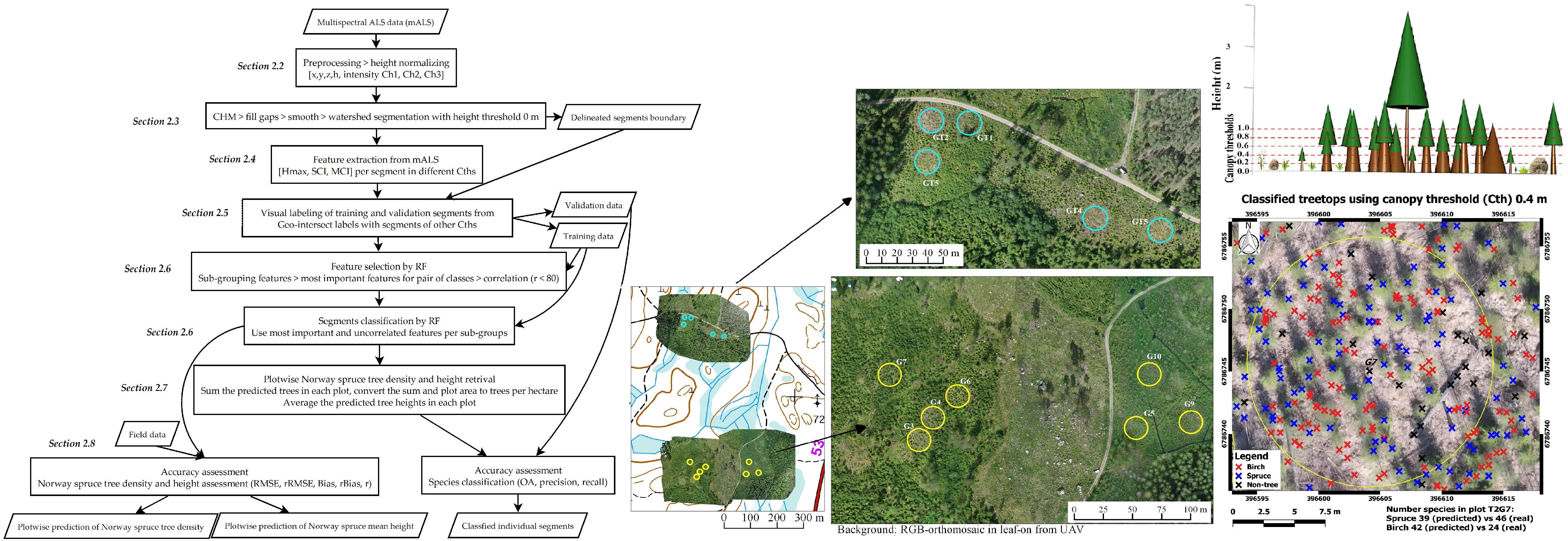
According to our findings, increasing C_th improved the accuracy of classification, which could be due to minimizing the effect of ground returns and removing low-height segments. This was clearly observed, as the C_th of 0 m yielded the worst results. Increasing C_th above 1 m also led to the omission of shorter seedlings; thus, we focused on optimizing C_th between 0 and 1 m.

The OA obtained with SCI-Ch1 and SCI-Ch2 when using the highest C_th (1 m) in leaf-off condition were 87.36% and 82.76%, respectively, whereas a higher OA of 83.70% was already achieved when using MCI with the lowest C_th (0 m; Table 6). A similar pattern was observed in the leaf-on condition. We concluded that using mALS makes it possible to perform detections with a smaller C_th compared to both SCI-Ch1 and SCI-Ch2, due to the higher efficiency of mALS compared to SCI-Ch1 and SCI-Ch2 in the classification of vegetation. mALS demonstrated more reliable potential for classification compared to both SCI-Ch1 and SCI-Ch2 in characterizations of small seedlings.

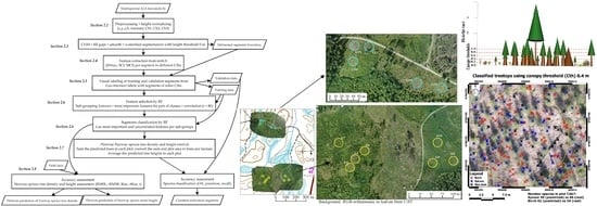
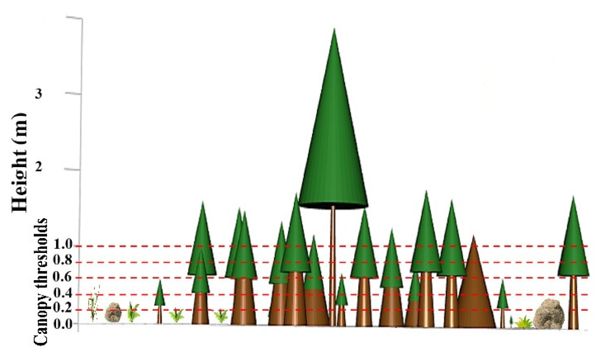
4.2. Tree Density Estimation

Dense point clouds from ALS, processed with the ITD method, produced accurate density estimates of the seedling stands. The tree density of Norway spruce seedlings was most accurately predicted in leaf-off data using a C_th 0.4 m (rRMSE: 37.9%). Our results also showed that mALS data outperformed in leaf-off compared to leaf-on for tree density estimation of Norway spruce seedlings.

The ITD method (watershed segmentation) was used to detect tree crowns in this study, which, to the best of our knowledge, has not yet been employed in characterizing seedling stands using ALS data. Two similar studies in seedling stands using ALS data with the ABA method in tree density estimation of seedling stands reported rRMSE values of 53.4% and 42%, respectively [9,27]. The improvement in accuracy achieved in this study could be firstly attributed to the use of the ITD method; secondly, the higher point density (~57 points/m²) used in this work compared to those of approximately 5 and 1.2 points/m² applied in the two other studies, respectively, would be expected to improve the estimates. Therefore, dense point clouds from mALS can also enhance tree detection in seedling stands. Notably, the increase in accuracy in leaf-off conditions can be attributed to the higher point density (60.10 points/m²) than in leaf-on (57.17 points/m²).

Another seedling stands study at the stand level used low-density (~0.7 points/m²), single-channel ALS with the ABA method and predicted the total tree density with an rRMSE of 47% [26]. According to Puliti et al. [9], a decrease in RMSE occurs when plot-level estimates are scaled to the stand level. Korhonen et al. [29] reported that using stand-level ABA with ALS usually results in higher accuracy than plot-level estimates, because random errors cancel each other out. Therefore, as our tree density estimation was at the plot level, the achieved rRMSE of 37.9% compared to the rRMSE of 47% obtained in the study of Ørka et al. [26] at the stand level further endorses the capability of the dense mALS data processed with the ITD method in this study. Our method also pursues plot-level estimations because more dense ALS data are becoming available.

Tree density estimation was more accurately predicted in AdS than YoS (Table 7), potentially because the shortest tree in AdS (minimum height of 1.57 m) was above the highest C_th (1 m) used. Therefore, theoretically, selecting any C_th (0–1 m), no trees were cut out in AdS for the classification phase, because all trees were already above 1 m. The situation was different in YoS, where the tree height ranged from 0.73 to 1.87 m, overlapping the C_th range and allowing the change in C_th to affect the tree density estimation by omitting trees shorter than the applied C_th (Table 1).

The sharp treetops in both YoS and AdS lowered the chance of being hit by the laser. In YoS, however, the treetops fell within the range of the applied C_th, whereas in AdS, the treetops were already above all the C_th values, which caused the omission of treetops to be more influential in YoS, resulting in higher underestimation of tree density as C_th increased. Note that when C_th was smaller, overestimation was observed. Therefore, according to our C_th optimization, the most accurate tree density in YoS was obtained with a C_th of 0.4 m (rRMSE: 46.49% and rBias: −28.78%). In AdS, however, 1 m was the optimum C_th both in leaf-off and leaf-on conditions (rRMSE 6.23% and 18.33%, respectively). Therefore, applying a C_th of 1 m is recommended for seedling stands with minimum height above 1.5 m, as supported by our results for AdS.

Our tree density estimation in AdS and YoS outperformed the values reported by Imangholiloo et al. [7], who used the same ITD method as ours and UAV-PPC and hyperspectral data. They reported rRMSE values of 19.2% and 58.2% for AdS and YoS in leaf-on data, respectively. In this study, we obtained an rRMSE of 6.23% with a C_th of 1.0 m for AdS, and an rRMSE of 46.49% in YoS with a C_th of 0.4 m, both in leaf-off. The better results in this research may be due to the dense point clouds and the penetration of ALS inside the canopy, especially in dense plots.

In our characterizations of seedling stands, we achieved almost the same rRMSE using ALS as studies using UAVs. For example, Puliti et al. [9] and Imangholiloo et al. [7] reported rRMSE values of 36.3% and 38.1% using ABA and ITD methods, respectively. Reaching the same accuracy (rRMSE 37.9% in leaf-off, C_th 0.4 m) reflects the superior ability of ALS, i.e., it provides advantages in penetrating the canopy, and is independent of direct sunlight, clear sky, and the ITD method used in our study.

In this study, we assessed the effect of different C_th values. The results of C_th optimization suggested C_th values of 0.4 and 1.0 m for YoS and AdS, respectively, to estimate tree density. These values are almost equal with the selected C_th values of 0.5 and 1.0 m for YoS and AdS, respectively, in the UAV study of Imangholiloo et al. [7]. We also found a C_th of 0.4 m to be the optimum C_th for all plots, which was the same as that obtained in the ALS study by Korpela et al. [39], who selected a C_th of 0.4 m after testing C_th in the range of 0.1 to 0.5 m. Ørka et al. [26] also used three C_th values of 0, 0.5, and 1.0 m, employing ALS to predict tree density in regeneration forests. They achieved the most accurate tree density estimation using a 0.5 m C_th.

In our study, misclassification of nontrees (especially bushes and grasses) as Norway spruces also affected the tree density estimation. For instance, with a C_th of 0.4 m, the leaf-off data commissions (precision) of birch, Norway spruce, and nontree classes were 0.89%, 1.00%, and 0.67%, respectively (results not shown). Carefully checking the confusion matrix of the data, in the validation data (92 segments), all Norway spruces (58) were correctly classified; however, one nontree and one birch segment were misclassified as Norway spruce, leading to overestimation of Norway spruce tree density (rBias: −23.44%).

4.3. Tree Height Estimation

Dense point clouds from mALS analyzed with ITD methods produced highly accurate height estimation in seedling stands. The height of Norway spruce was most accurately predicted in leaf-on data using a C_th of 0.2 m (rRMSE: 10.76%). The novel use of leaf-off and leaf-on mALS data in seedling stands demonstrated that leaf-on data outperformed leaf-off data for tree height estimation of Norway spruce seedlings.

A few studies have assessed trees height in seedling stands using ALS data with ABA methods. The heights of seedling stands were reported with rRMSEs of 28% [26] and 32.0% [9] at the stand and plot levels, respectively. The improvement in height estimation accuracy achieved in this study could mainly be attributed to the higher point density (~57 points/m²) used in our research compared to the point density of approximately 0.7 and 5 points/m² applied in the two others, respectively. Therefore, dense point clouds from ALS also enhance the tree height estimation in seedling stands studies. In addition to the dense point clouds used, the difference could also be due to the ITD method used in this study.

The tree height was underestimated by 6.88% in leaf-on data with a C_th of 0.2 m. Korpela et al. [28] also used the ITD method with leaf-on ALS and aerial imagery in seedling stands, and obtained underestimations of tree height of between 20% and 40%. Their study area was more complex (i.e., higher tree density and classification classes) than that in this study. The point density of 57.17 points/m² used in this study was higher than theirs, i.e., 6–9 points/m², and they used spectral data from aerial images instead of our use of intensity data from mALS.

Two similar studies, Vepakomma et al. [8] and Imangholiloo et al. [7], using the ITD method and UAV-PPC data instead of ALS, underestimated height by 0.39 and 0.16 m (6.90%), respectively. Reaching the same accuracy (bias: 0.16 m in leaf-on, C_th 0.2 m) reflects the superior ability of ALS, as it operates independent of direct sunlight and clear sky. Goodbody et al. [15] and Puliti et al. [9] applied UAV in seedling studies using OBIA and ABA methods, achieving an RMSE of 0.92 m and an rRMSE of 30.9%, respectively. The improvement (RMSE: 0.25 m and rRMSE: 10.76% in leaf-on, C_th 0.2 m) could be due to the ITD method and the dense point clouds used in this study.

In terms of optimum C_th for tree height estimation, the C_th values of 0.2 m, and 0.2, and 0.6 m were found to be optimal for YoS and AdS, respectively. These values are lower than the 0.5 and 1.0 m C_th values for YoS and AdS, respectively, selected by Imangholiloo et al. [7]. Similarly, in terms of optimum C_th among all plots, the C_th of 0.2 m in this study was lower than the 0.4 m used by Korpela et al. [28]. The lower C_th could be due to the remaining (correctly classified) tall spruces, thereby increasing the mean plot height. Ørka et al. [26] used three C_th values of 0, 0.5, and 1.0 m for ALS point clouds to predict tree-height-related attributes in regeneration forests. They achieved the most accurate height estimation with a C_th of 0 m, which is close to the C_th value of 0.2 m in our study.

Another factor potentially influencing height estimation is the accuracy of Näslund’s model in predicting heights of field data, as well as the accuracy of the DTM used for the height normalization of ALS point clouds. If tree height is measured at the individual tree level during field surveys, Näslund’s model would not be needed and the ALS-estimated tree heights could be assessed at the individual tree and plot levels. More important than the previously mentioned factors, possible tree height growth between leaf-off ALS data acquisitions and field data collection (time lag was about 45 days) could have caused the higher underestimation of height in leaf-off than in leaf-on conditions.

Another issue in the tree height estimations of YoS was their higher vulnerability to the influence of DTM errors compared to AdS. When height normalization of point clouds was conducted, we assumed that errors affected over- or under- estimations of YoS heights more than for AdS. To illustrate, if DTM has a 20 cm error, for example, its proportional error to a tree with a height of 1 m (20%) would be higher than for a tree with a height of 20 m (1%). As a result, the error in DTM for height normalization can influence tree density estimation, especially for YoS. This consequently affects height estimation, because trees are relatively smaller in YoS than AdS; hence, the error in the DTM influences the estimation proportional to their short height more significantly.

4.4. Comparing Leaf-Off and Leaf-On Data

We observed that the mALS data acquired in leaf-off conditions produced the most accurate estimates for classification and tree density. Leaf-on data produced more accurate results for tree height estimation.

For classification in leaf-off and leaf-on conditions, the advantage seen from the use of leaf-off data in this study was in line with the findings of Kim et al. [40], who used leaf-off and leaf-on ALS data for species classification of mature broadleaved and coniferous trees. Their leaf-off data yielded a higher OA (83.4%) than leaf-on data (73.1%). The outperformance of leaf-off ALS data was supported by other studies that used Optech Titan mALS data for species classification of trees in mature forests [31,38]. The more accurate OA in the leaf-off condition in our study may have occurred because coniferous trees are green in leaf-off, while other classes (birch, grass, etc.) are leafless. Therefore, the classification was easier in leaf-off than in leaf-on conditions, in which both tree species (Norway spruce and birch) and nontree classes were green, and harder to separate. Leaf-off MCI data were more favorable for classification than leaf-on because the interference of grass and bushes was eliminated in the leaf-off condition. Classification was closely related to the accuracy of estimating tree density; thus, leaf-off also produced more accurate results compared to leaf-on data.

In terms of height estimation of Norway spruce seedlings, leaf-on data yielded more accurate results. Compared with mature forests, leaf-off ALS data analyzed with ABA outperformed leaf-on data [41,42,43]. The decision to use leaf-off data was, however, in contrast with our findings that showed higher suitability of leaf-on data for height estimation. This finding could be due to height growth between leaf-off ALS data collection and field height measurement during leaf-on time (time lag of 45 days), as explained in Section 4.3.

5. Conclusions

The ability of mALS compared to single-channel ALS data to characterize tree attributes (species, density, and height) in seedling stands in YoS, AdS, and all plots was assessed in this study. The data were obtained in leaf-off and leaf-on conditions. The optimal C_th for each of the estimations was addressed separately.

According to our classification results, the MCI data produced more accurate results compared to both SCI-Ch1 and SCI-Ch2 for characterizations of small seedlings (YoS). The use of MCI data also allowed detection using a lower C_th compared to both SCI-Ch1 and SCI-Ch2. The reason for this finding probably lies in the higher efficiency of MCI than SCI in the detection of vegetation. It is critical to adjust C_th depending on the tree height in seedling stands, since, based on the results, the classification accuracy improved with increasing C_th.

Our results also demonstrated the capability of mALS for tree density estimations in seedling plots. The results were further improved with the use of the ITD method. A C_th of 0.4 m yielded the most accurate tree density estimation for all plots, whereas C_th values of 0.4 and 1.0 m yielded the best results for YoS and AdS, respectively. Overall, tree density was estimated more accurately in AdS compare to YoS, and in the leaf-off compared to the leaf-on condition. Leaf-on conditions, however, resulted in more accurate tree height estimates. The C_th of 0.2 m resulted in the most accurate tree height estimates for all plots, whereas C_th values of 0.2 and both 0.2 and 0.6 m resulted in the most accurate results for YoS and AdS, respectively. We concluded that mALS data are a reliable resource for undertaking RS-based inventories of seedling stands. Further research with a larger number of sample plots including diverse seedling species, densities, and heights is required. Generally, leaf-off data are recommended, since the data can additionally provide accurate DTMs, if not otherwise available.

References

1. Tapio. Hyvän Metsänhoidon Suositukset. (Recommendations for Forest Management in Finland); Forest Development Centre Tapio. Metsäkustannus oy: Helsinki, Finland, 2006; p. 100. (In Finnish) [Google Scholar]
2. Huuskonen, S.; Hynynen, J. Timing and intensity of precommercial thinning and their effects on the first commercial thinning in Scots pine stands. Silva Fenn. 2006, 40, 645–662. [Google Scholar] [CrossRef] [Green Version]
3. Uotila, K.; Saksa, T. Effects of early cleaning on young Picea abies stands. Scand. J. For. Res. 2014, 29, 111–119. [Google Scholar] [CrossRef]
4. Kangas, A.; Astrup, R.; Breidenbach, J.; Fridman, J.; Gobakken, T.; Korhonen, K.T.; Maltamo, M.; Nilsson, M.; Nord-Larsen, T.; Næsset, E.; et al. Remote sensing and forest inventories in Nordic countries–roadmap for the future. Scand. J. For. Res. 2018, 33, 397–412. [Google Scholar] [CrossRef] [Green Version]
5. Emondino, F.R.; Pera, M.G.S.; Ocerino, E.N.; Enna, F.M.; Ex, F.N. State of the art in high density image matching. Photogramm. Rec. 2014, 29, 144–166. [Google Scholar] [CrossRef] [Green Version]
6. Sedaghat, A.; Ebadi, H. Remote Sensing Image Matching Based on Adaptive Binning SIFT Descriptor. IEEE Trans. Geosci. Remote Sens. 2015, 53, 5283–5293. [Google Scholar] [CrossRef]
7. Imangholiloo, M.; Saarinen, N.; Markelin, L.; Rosnell, T.; Näsi, R.; Hakala, T.; Honkavaara, E.; Holopainen, M.; Hyyppä, J.; Vastaranta, M. Characterizing Seedling Stands Using Leaf-Off and Leaf-On Photogrammetric Point Clouds and Hyperspectral Imagery Acquired from Unmanned Aerial Vehicle. Forests 2019, 10, 415. [Google Scholar] [CrossRef] [Green Version]
8. Vepakomma, U.; Cormier, D.; Thiffault, N. Potential of UAV based convergent photogrammetry in monitoring regeneration standards. Int. Arch. Photogramm. Remote Sens. Spat. Inf. Sci.-ISPRS Arch. 2015, 40, 281–285. [Google Scholar] [CrossRef] [Green Version]
9. Puliti, S.; Solberg, S.; Granhus, A. Use of UAV Photogrammetric Data for Estimation of Biophysical Properties in Forest Stands Under Regeneration. Remote Sens. 2019, 11, 233. [Google Scholar] [CrossRef] [Green Version]
10. Green, P.C.; Burkhart, H.E. Plantation Loblolly Pine Seedling Counts with Unmanned Aerial Vehicle Imagery: A Case Study. J. For. 2020, 1–14. [Google Scholar] [CrossRef]
11. Fromm, M.; Schubert, M.; Castilla, G.; Linke, J.; McDermid, G. Automated detection of conifer seedlings in drone imagery using convolutional neural networks. Remote Sens. 2019, 11, 2585. [Google Scholar] [CrossRef] [Green Version]
12. Kingstad, V. Evaluated Density Estimates of Young Forest Stands Using High Resolution 2D Imagery from UAV; Swedish University of Agricultural Sciences: Uppsala, Sweden, 2020. [Google Scholar]
13. White, R.; Bomber, M.; Hupy, J.; Shortridge, A. UAS-GEOBIA Approach to Sapling Identification in Jack Pine Barrens after Fire. Drones 2018, 2, 40. [Google Scholar] [CrossRef] [Green Version]
14. Feduck, C.; McDermid, G.J.; Castilla, G. Detection of coniferous seedlings in UAV imagery. Forests 2018, 9, 432. [Google Scholar] [CrossRef] [Green Version]
15. Goodbody, T.R.H.; Coops, N.C.; Hermosilla, T.; Tompalski, P.; Crawford, P. Assessing the status of forest regeneration using digital aerial photogrammetry and unmanned aerial systems. Int. J. Remote Sens. 2018, 00, 1–19. [Google Scholar] [CrossRef]
16. Kirby, C.L. A Camera and Interpretation System for Assessment of Forest Regeneration; Environment Canada, Canadian Forestry Service; Northern Forest Research Centre: Edmonton, AB, USA, 1980. [Google Scholar]
17. Hall, R.J.; Aldred, A.H. Forest regeneration appraisal with large-scale aerial photographs. For. Chron. 1992, 68. [Google Scholar] [CrossRef] [Green Version]
18. Pouliot, D.A.; King, D.J.; Pitt, D.G. Automated assessment of hardwood and shrub competition in regenerating forests using leaf-off airborne imagery. Remote Sens. Environ. 2006, 102, 223–236. [Google Scholar] [CrossRef]
19. Pouliot, D.A.; King, D.J.; Pitt, D.G. Development and evaluation of an automated tree detection—Delineation algorithm for monitoring regenerating coniferous forests. Can. J. For. Res. 2005, 35, 2332–2345. [Google Scholar] [CrossRef] [Green Version]
20. Vastaranta, M.; Wulder, M.A.; White, J.C.; Pekkarinen, A.; Tuominen, S.; Ginzler, C.; Kankare, V.; Holopainen, M.; Hyyppä, J.; Hyyppä, H. Airborne laser scanning and digital stereo imagery measures of forest structure: Comparative results and implications to forest mapping and inventory update. Can. J. Remote Sens. 2013, 39, 382–395. [Google Scholar] [CrossRef]
21. Petrie, G.; Toth, C.K. Introduction to Laser Ranging, Profiling, and Scanning. In Topographic Laser Ranging and Scanning: Principles and Processing; Shan, J., Toth, C.K., Eds.; Taylor & Francis Group: Boca Raton, FL, USA, 2009; pp. 1–27. [Google Scholar]
22. Hauglin, M.; Bollandsås, O.M.; Gobakken, T.; Næsset, E. Monitoring small pioneer trees in the forest-tundra ecotone: Using multi-temporal airborne laser scanning data to model height growth. Environ. Monit. Assess. 2018, 190. [Google Scholar] [CrossRef]
23. Thieme, N.; Bollandsa, O.M.; Gobakken, T.; Næsset, E. Detection of small single trees in the forest tundra ecotone using height values from airborne laser scanning. Can. J. Remote Sens. 2011, 37, 264–274. [Google Scholar] [CrossRef]
24. Næsset, E. Estimating above-ground biomass in young forests with airborne laser scanning. Int. J. Remote Sens. 2011, 32, 473–501. [Google Scholar] [CrossRef]
25. Økseter, R.; Bollandsås, O.M.; Gobakken, T.; Næsset, E. Modeling and predicting aboveground biomass change in young forest using multi-temporal airborne laser scanner data. Scand. J. For. Res. 2015, 30, 458–469. [Google Scholar] [CrossRef]
26. Ørka, H.O.; Gobakken, T.; Næsset, E. Predicting Attributes of Regeneration Forests Using Airborne Laser Scanning. Can. J. Remote Sens. 2016, 42, 541–553. [Google Scholar] [CrossRef]
27. Næsset, E.; Bjerknes, K.O. Estimating tree heights and number of stems in young forest stands using airborne laser scanner data. Remote Sens. Environ. 2001, 78, 328–340. [Google Scholar] [CrossRef]
28. Korpela, I.; Tuomola, T.; Tokola, T.; Dahlin, B. Appraisal of seedling stand vegetation with airborne imagery and discrete-return LiDAR - an exploratory analysis. Silva Fenn. 2008, 42, 753–772. [Google Scholar] [CrossRef] [Green Version]
29. Korhonen, L.; Pippuri, I.; Packalén, P.; Heikkinen, V.; Maltamo, M.; Heikkilä, J. Detection of the need for seedling stand tending using high-resolution remote sensing data. Silva Fenn. 2013, 47, 1–20. [Google Scholar] [CrossRef] [Green Version]
30. Gorgens, E.B.; Valbuena, R.; Rodriguez, L.C.E. A method for optimizing height threshold when computing airborne laser scanning metrics. Photogramm. Eng. Remote Sens. 2017, 83, 343–350. [Google Scholar] [CrossRef]
31. Yu, X.; Hyyppä, J.; Litkey, P.; Kaartinen, H.; Vastaranta, M.; Holopainen, M. Single-Sensor Solution to Tree Species Classification Using Multispectral Airborne Laser Scanning. Remote Sens. 2017, 9, 108. [Google Scholar] [CrossRef] [Green Version]
32. Näslund, M. Skogsförsöksanstaltens Gallringsförsök i Tallskog; Meddelanden från Statens skogsförsöksanstalt (0283-3093); Statens Skogsförsöksanstalt: Stockholm, Sweden, 1936; p. 169. [Google Scholar]
33. Hijmans, R.J. Raster: Geographic Data Analysis and Modeling. R Package Version 2.6-7. 2017. Available online: https://CRAN.R-project.org/package=raster (accessed on 14 September 2020).
34. Breiman, L. Random forests. Mach. Learn. 2001, 45, 5–32. [Google Scholar] [CrossRef] [Green Version]
35. Pedregosa, F.; Varoquaux, G.; Gramfort, A.; Michel, V.; Thirion, B.; Grisel, O.; Blondel, M.; Prettenhofer, P.; Weiss, R.; Dubourg, V.; et al. Scikit-learn: Machine Learning in Python. J. Mach. Learn. Res. 2011, 12, 2825–2830. [Google Scholar]
36. Budei, B.C.; St-Onge, B.; Hopkinson, C.; Audet, F.A. Identifying the genus or species of individual trees using a three-wavelength airborne lidar system. Remote Sens. Environ. 2018, 204, 632–647. [Google Scholar] [CrossRef]
37. Shi, Y.; Wang, T.; Skidmore, A.K.; Heurich, M. Important LiDAR metrics for discriminating forest tree species in Central Europe. ISPRS J. Photogramm. Remote Sens. 2018, 137, 163–174. [Google Scholar] [CrossRef]
38. Axelsson, A.; Lindberg, E.; Olsson, H. Exploring multispectral ALS data for tree species classification. Remote Sens. 2018, 10, 183. [Google Scholar] [CrossRef] [Green Version]
39. Korpela, I.; Hovi, A.; Morsdorf, F. Understory trees in airborne LiDAR data—Selective mapping due to transmission losses and echo-triggering mechanisms. Remote Sens. Environ. 2012, 119, 92–104. [Google Scholar] [CrossRef]
40. Kim, S.; McGaughey, R.J.; Andersen, H.E.; Schreuder, G. Tree species differentiation using intensity data derived from leaf-on and leaf-off airborne laser scanner data. Remote Sens. Environ. 2009, 113, 1575–1586. [Google Scholar] [CrossRef]
41. White, J.C.; Arnett, J.T.T.R.; Wulder, M.A.; Tompalski, P.; Coops, N.C. Evaluating the impact of leaf-on and leaf-off airborne laser scanning data on the estimation of forest inventory attributes with the area-based approach. Can. J. For. Res. 2015, 45, 1498–1513. [Google Scholar] [CrossRef] [Green Version]
42. Villikka, M.; Packalén, P.; Maltamo, M. The suitability of leaf-off airborne laser scanning data in an area-based forest inventory of coniferous and deciduous trees. Silva Fenn. 2012, 46, 99–110. [Google Scholar] [CrossRef] [Green Version]
43. Ørka, H.O.; Næsset, E.; Bollandsås, O.M. Effects of different sensors and leaf-on and leaf-off canopy conditions on echo distributions and individual tree properties derived from airborne laser scanning. Remote Sens. Environ. 2010, 114, 1445–1461. [Google Scholar] [CrossRef]
Figure 1. Map of the study area and established sample plots in young seedling stand (upper image block) and in advanced seedling stand (lower image block).
Remotesensing 12 03328 g001
Figure 2. A flowchart outlining the methodology. Text sections are noted on the left.
Remotesensing 12 03328 g002
Figure 3. A simplified schematic illustrating canopy thresholds (Cths).
Remotesensing 12 03328 g003
Figure 4. Box-whisker plots of the selected most important and uncorrelated features (green-colored features in Table 5). The boxes show the mean and first and third quantiles in the box, as well as the minimum and maximum values in line, using validation data with a canopy threshold (Cth) of 0.4 m in leaf-off (A) and leaf-on (B) conditions. Features of single- and multi- channel intensity (SCI and MCI, respectively) data are plotted in left and right, respectively. Explanations for features are provided in Table 4.
Remotesensing 12 03328 g004
Figure 5. Classified treetops in an advanced seedling plot using leaf-off data in canopy threshold (Cth) of 0.4 m (background is RGB orthomosaic in leaf-off from UAV with resolution of 2.5 cm).
Remotesensing 12 03328 g005
Figure 6. Tree density (unit: tree per hectare) of Norway spruce seedlings in leaf-off (a) and leaf-on (b) conditions, separating plots in young seedling stand (YoS, n = 5) and advanced seedling stand (AdS, n = 7) in canopy thresholds of 0.4 m.
Remotesensing 12 03328 g006
Figure 7. Height (unit: meter) of Norway spruce seedlings in leaf-off (a) and leaf-on (b) conditions, separating plots in young seedling stand (YoS, n = 5) and advanced seedling stand (AdS, n = 7) in canopy thresholds of 0.2 m.
Remotesensing 12 03328 g007