A Refinement Method of Real-Time Ionospheric Model for China

Abstract

Ionospheric delay is a crucial error source and determines the source of single-frequency precise point positioning (SF-PPP) accuracy. To meet the demands of real-time SF-PPP (RT-SF-PPP), several international global navigation satellite systems (GNSS) service (IGS) analysis centers provide real-time global ionospheric vertical total electron content (VTEC) products. However, the accuracy distribution of VTEC products is nonuniform. Proposing a refinement method is a convenient means to obtain a more accuracy and consistent VTEC product. In this study, we proposed a refinement method of a real-time ionospheric VTEC model for China and carried out experiments to validate the model effectiveness. First, based on the refinement method and the Centre National d’Études Spatiales (CNES) VTEC products, three refined real-time global ionospheric models (RRTGIMs) with one, three, and six stations in China were built via GNSS observations. Second, the slant total electron content (STEC) and Jason-3 VTEC were used as references to evaluate VTEC accuracy. Third, RT-SF-PPP was used to evaluate the accuracy in the positioning domain. Results showed that even if using only one station to refine the global ionospheric model, the refined model achieved a better performance than CNES and the Center for Orbit Determination in Europe (CODE). The refinement model with six stations was found to be the best of the three refinement models.

1. Introduction

In recent years, the use of GNSS has gradually increased in geodesy, deformation monitoring, precision agriculture, hazard monitoring, and vehicle navigation fields [1,2,3,4]. Applications of different positioning accuracy require different positioning strategies. Differential positioning can eliminate orbit error, clock error, receiver clock error, and weaken ionosphere and troposphere errors, thus becoming a widely used technology in the application of high-precision positioning [5,6]. However, differential positioning is inconvenient and high-cost because it relays simultaneous observations at the reference station [3,7]. Precision point positioning (PPP) does not rely on a reference station. Rather, it derives centimeter to decimeter level positioning accuracy using a single receiver in support of precision orbit and clock products [3,8,9]. Recently, consumer requirements of high precision positioning has gradually increased [4]. Real-time single-frequency PPP (RT-SF-PPP) has become a desired consumer positioning approach because it has more advantages like low-cost, low bandwidth, and no base station required when compared to real-time differential (RTD) positioning [10].

RT-SF-PPP requires real-time precise orbit, clock products, and real-time ionospheric products [10,11]. The IGS officially launched real-time service (RTS) on 1 April 2013, providing real-time satellite orbit and clock products [12]. Several RTS products are also available from real-time analysis centers (ACs) like the Centre National d’Études Spatiales (CNES), the Bundesamt für Kartographie und Geodäsie (BKG), and Wuhan University (WHU). Extensive research has been carried out to evaluate the performance of real-time precise orbits and clocks products, showing that accuracy of orbits and clocks can reach the centimeter-level and satisfy real-time PPP requirements [8,12,13]. As real-time high precise orbits and clocks products become available, ionospheric delay error emerges as the primary error of RT-SF-PPP [11,14].

To date, several real-time ionospheric vertical total electron content (VTEC) products have been accessed via the internet. CNES is the first institute broadcasting ionospheric VTEC message through its RTS streams [10]. Moreover, IGS analysis centers (ACs)—e.g., WHU, the Chinese Academy of Sciences (CAS), Universitat Politècnica de Catalunya (UPC)—provide real-time ionospheric VTEC products [11,15]. Performance evaluation shows that the accuracy of real-time ionospheric VTEC products reaches 2–5 total electron content unit (TECU) and the average accuracy of SF-PPP reaches a submeter level [10,11,15].

However, the evaluations mostly reflect the average accuracy of global ionospheric VTEC products. Real-time modeling of ionospheric VTEC product relies on real-time GNSS stations. Because IGS GNSS stations are distributed unevenly, the accuracy of ionospheric VTEC is nonuniform. The area of China is similar to North American and Europe. Nevertheless, there are only two real-time IGS GNSS stations. Moreover, once the real-time data stream becomes unstable, fewer stations can be used in real-time global modeling. Along with China’s fast development, the number of RT-SF-PPP users will be very large-scale in the future. Thus, improving the accuracy of real-time VTEC products in China is required.

Based on regional the GNSS network, various regional VTEC models have been proposed [16,17,18,19], which will have a better performance than the global VTEC product. However, model representation is considerable in real-time GNSS applications because the positioning terminal should keep consistency with the VTEC model. Due to the universal use of CNES VTEC products, proposing a refinement method becomes a convenient means for improving the regional accuracy for China.

In this paper, we proposed a regional refinement method based on CNES ionospheric VTEC products for China, and evaluated the performance of primary results. First, we introduce the data and materials used in this study. Then, the refinement method is proposed to update ionospheric spherical harmonic coefficients. Moreover, experiments of the refinement modeling were carried out and the performance of the primary results was evaluated.

To demonstrate the advantage of the refinement models, CNES and CODE models are also evaluated as well. Because local GNSS stations are utilized, the advantage of the refinement models is having a higher accuracy in and around China. Meanwhile, the weaknesses of the global VTEC models like CNES and CODE is the low accuracy in the region because of the lack of GNSS stations. To evaluate the accuracy of the VTEC models, external ionospheric data, namely slant total electron content (STEC) from dual-frequency measurements and VTEC from Jason-3, are used as references. The accuracy of STEC derived by the carrier phase smoothed code method can reach to 0.2–0.4 TECU [20], which is enough to be a reference. Meanwhile, VTEC data from Jason-3 are a widely used external data source to evaluate global ionospheric model [11,21]. We collected 12 GNSS stations’ data in China and 22 days of Jason-3 VTEC data around China for the comparisons, which can demonstrate well the local accuracy of the VTEC models. Performance evaluation was carried out in three steps: (1) residual error analysis of refinement modeling, (2) comparison with external ionospheric total electron content (TEC) data, and (3) performance analysis of RT-SF-PPP. Summaries and conclusions are provided in the last section.

2. Data and Materials

2.1. Real-Time Global Ionosphere Model (GIM) Product of CNES

CNES is an IGS real-time analysis center (AC) [8,13] that developed precise point positioning with an integer and zero-difference ambiguity resolution demonstrator (PPP-WIZARD) project, which generated and broadcasted real-time state space representation (SSR) messages. The zero-difference ambiguity method was carried out in PPP-WIZARD to determine orbits and clocks of GNSS satellites using a global network of real-time GNSS stations. The core of the real-time process was a Kalman filter. In the Kalman filter, orbit/clock corrections, code bias, phase biases, and ionosphere VTEC were estimated in real-time. Four real-time service (RTS) streams of CNES—i.e., CLK90, CLK91, CLK92, and CLK93—were available for public access. For the four streams, CLK90 and CLK92 referred to the center of mass (CoM), whereas CLK91 and CLK93 referred to the antenna phase center (APC) [10]. All four streams contained ionospheric VTEC messages. We investigated CLK93 in this study.

Table 1. Messages provided by CLK93.

Constellation	Product	Occurrence (s)
GPS	Orbits/clocks/code biases/phase biases	5
GLONASS	Orbits/clocks/code biases	5
Galileo	Orbits/clocks/code biases/phase biases	5
BDS	Orbits/clocks/code biases/phase biases	5
/	Ionosphere VTEC	60

lists messages of CLK93. Orbits, clocks, code biases, phase biases, and VTEC messages were included. The update interval of VTEC is 60 s and the others are 5 s.

The ionospheric VTEC product is expressed by spherical harmonic expansions for each layer [10]:

$$VTEC\left({\varphi }_{IPP},{\lambda }_s\right)={\sum }_{n=0}^N{\sum }_{m=0}^{\min \left(n,M\right)}{P}_{nm}\left(C_{nm}\cos m{\lambda }_s+S_{nm}\sin m{\lambda }_s\right),$$

(1)

where $N$ and $M$ are the degree and order of the spherical harmonic expansions; $n$ and $m$ are the corresponding indices; $C_{nm}$ and $S_{nm}$ are the cosine and sine coefficients for the layer; ${\varphi }_{IPP}$ is the geocentric latitude of ionospheric pierce point (IPP) for the layer; ${\lambda }_s$ denotes the mean sun-fixed and phase-shifted longitude of IPP for the layer; and $P_{nm}={\tilde{P}}_{nm}\left(\sin {\varphi }_{IPP}\right)$ is the fully normalized associated Legendre function. The mean sun-fixed and phase-shifted longitude ${\lambda }_s$ is given by:

$${\lambda }_s={\lambda }_{IPP}+\frac{t-50400}{43200}\pi ,$$

(2)

where ${\lambda }_{IPP}$ is the longitude of IPP for the layer and $t$ is the universal time (UT) of observation epoch. Once VTEC is obtained, STEC can be computed by VTEC and the mapping function:

$$STEC=\frac{VTEC}{mf}=\frac{VTEC}{\cos Z_{ipp}},$$

(3)

About 100 real-time IGS GNSS stations were used in the real-time ionospheric VTEC model. The order of spherical harmonic moved from 6 to 12 on May 29, 2018. Quality assessment results showed that the root mean square errors (RMSE) of CNES varied from 2 to 6 TECU [10,11]. The accuracy of VTEC was nonuniform because the real-time GNSS stations were uneven for different regions. Some regions like Western Europe and North America are covered with reference stations. Nevertheless, in regions like Asia, Africa, Latin America, and other sea areas, IGS stations are sparse.

2.2. GNSS Stations for Refinement Modeling and Validation

In this study, three refinement models with different station counts were built and analyzed. The stations used by different models are listed in

Table 2. Global navigation satellite systems (GNSS) stations used for refinement modeling.

RRTGIM-1	RRTGIM-3	RRTGIM-6
HKSL	HKSL, B023, BJNM	HKSL, B023, BJNM, JFNG, J002, B018

. The first model was the refined real-time global ionospheric model with one station (RRTGIM-1), which only used one station named HKSL. RRTGIM-3 used three stations: HKSL, B023, and BJNM. For RRTGIM-6, six stations were used, i.e., HKSL, B023, BJNM, JFENG, J002, and B018. The distribution of these stations is shown in Figure 1. The observation data from day of year (DOY) 78 to 99, 2020, were collected for modeling. The recorded GNSS constellation, sample rate, receiver, and antenna of these stations are listed in

Table 3. Sample rate, constellation, receiver, and antenna of refinement GNSS stations.

Site	Sample Rate (s)	Constellation	Receiver	Antenna
BJFS	30	GPS + GLONASS	TRIMBLE NETR9	TRM59900.00
BJNM	30	GPS + GLONASS + Galileo	SEPT POLARX3ETR	NOV702GG
HKSL	30	GPS + GLONASS	LEICA GR50	LEIAR25.R4
J002	15	GPS + GLONASS	SINOGNSS M300	HARXON GPS1000
B018	15	GPS + GLONASS	SINOGNSS M300	HARXON GPS1000
B023	15	GPS + GLONASS	SINOGNSS M300	HARXON GPS1000

.

STEC from 24 stations, including 12 GNSS stations in China and 12 IGS GNSS stations from across the world, were selected as references to assess the accuracy of the refinement models. The distribution of the 24 stations is shown in Figure 2. The 12 stations in China validated the accuracy of the RRTGIM product in China, while the other 12 global stations were used to validate the refinement influence on other regions. The recorded GNSS constellations, sample rate, receiver, and antenna of the 12 validation stations in China are collected and listed in

Table 4. Sample rate, constellation, receiver, and antenna of validation stations.

Site	Sample Rate (s)	Constellation	Receiver	Antenna
B005	15	GPS + GLONASS	SINOGNSS M300	HARXON GPS1000
B016	15	GPS + GLONASS	SINOGNSS M300	HARXON GPS1000
B019	15	GPS + GLONASS	SINOGNSS M300	HARXON GPS1000
B026	15	GPS + GLONASS	SINOGNSS M300	HARXON GPS1000
B027	15	GPS + GLONASS	SINOGNSS M300	HARXON GPS1000
B031	15	GPS + GLONASS	SINOGNSS M300	HARXON GPS1000
B081	15	GPS + GLONASS	SINOGNSS M300	HARXON GPS1000
B083	15	GPS + GLONASS	SINOGNSS M300	HARXON GPS1000
B085	15	GPS + GLONASS	SINOGNSS M300	HARXON GPS1000
HKNP	30	GPS + GLONASS	LEICA GR50	LEIAR25.R4
HKKT	30	GPS + GLONASS	LEICA GR50	LEIAR25.R4
JFNG	30	GPS + GLONASS	TRIMBLE NETR9	TRM59800.00

. The information for the IGS stations is omitted here.

2.3. Jason-3 VTEC Product for Comparison

VTEC of Jason-3 was adopted as a reference to evaluate refinement products, CNES, and CODE. Jason-3 was launched on 17 January 2016 [21,22]. The objective was to provide high accuracy data for ocean streams and sea levels. VTEC were derived from Ku-band ionospheric corrections:

$$VTEC=-dR\frac{f_{Ku}^2}{40.3},$$

(4)

where $dR$ is the ionospheric correction and $f_{Ku}$ is the frequency of Ku-band in GHz.

The data points of Jason-3 VTEC in cycle 152 are dotted in Figure 3, colored by CODE differences. As shown in Figure 3, most data points were distributed in the ocean area because Jason-3 only received rays reflected from the water. The average bias was 1.72 TECU and the RMSE was 4.93 TECU, which showed that CODE differences were minor. Twenty-two days of Jason-3 VTEC products between DOY 78 to 99, 2020, in region 97–127° E, 18–45° N were extracted as the reference for our study.

3. Methodology

The procedure of refinement modeling is shown in Figure 4. As shown in the figure, CLK93 SSR messages, including ionospheric VTEC coefficient, clock corrections, orbit corrections, code bias, and phase bias, are received and decoded via the SGGNtrip client, which is a RTCM networked transport via an Internet protocol (NTRIP) client developed at the School of Geodesy and Geomatics (SGG), Wuhan University [14]. There are four steps required to conduct the refinement:

(a)

Calculate the precise orbit using orbit SSR messages and broadcast (BRDC) ephemeris [8,12];

(b)

Calculate the position of IPP using satellite coordinates and GNSS station position [10] (note that the accuracy of the broadcast orbit is enough to calculate the position of IPP because orbit corrections are not strictly necessary);

(c)

Calculate STEC using GNSS dual-frequency measurements [10,23];

(d)

Refining the CNES ionospheric VTEC model using the refinement method.

3.1. Method to Determine STEC

Two methods were utilized to derive ionospheric STEC: the carrier-phase smoothed code method and PPP with raw observation method [23,24]. Because it is easy to conduct the carrier-phase smoothed code method, we used it to demonstrate the refinement in this study.

The GNSS observation equation can be expressed as

$$P_{k,j}^i={\rho }_j^i+c\left({\tau }^i-{\tau }_j\right)+d_k^i+d_{k,j}+Io{n}_{k,j}^i+Tro{p}_j^i+{\epsilon }_{P,k,j}^i,$$

(5)

$$L_{k,j}^i={\rho }_j^i+c\left({\tau }^i-{\tau }_j\right)+\lambda \left(b_{k,j}^i+N_{k,j}^i\right)-Io{n}_{k,j}^i+Tro{p}_j^i+{\epsilon }_{L,k,j}^i$$

(6)

where superscript $i$ and subscripts $k$ and $j$ denote specific satellites, frequencies, and receivers; $P_{k,j}^i$ and $L_{k,j}^i$ are the code and phase observations; ${\rho }_j^i$ is the geometric distance from the satellite to the receiver; $c$ denotes the speed of light; ${\tau }^i$ is the satellite clock error; ${\tau }_j$ is the receiver clock error; $Io{n}_{k,j}^i$ and $Tro{p}_j^i$ are ionospheric delay and tropospheric delay; $d_k^i$ and $d_{k,j}$ are satellite and receiver code biases; $b_{k,j}^i$ is the phase biases; $N_{k,j}^i$ is the ambiguity of the carrier phase; and ${\epsilon }_{L,k,j}^i$ and ${\epsilon }_{P,k,j}^i$ are the residuals of phase and code in GNSS measurements.

With dual-frequency observations, the ionospheric delays can be obtained as follows:

$$P_4=P_{1,j}^i-P_{2,j}^i=\left(Io{n}_{1,j}^i-Io{n}_{2,j}^i\right)+DC{B}^i+DC{B}_j,$$

(7)

$$L_4=L_{1,j}^i-L_{2,j}^i=-\left(Io{n}_{1,j}^i-Io{n}_{2,j}^i\right)+\lambda \left(b_{1,j}^i-b_{2,j}^i\right)+\lambda \left(N_{1,j}^i-N_{2.j}^i\right)$$

(8)

where $DC{B}^i=d_1^i-d_2^i$ and $DC{B}_j=d_{1,j}-d_{2,j}$ stand for differential code biases of the satellites and differential code biases of the receivers, respectively.

As the code observation $P_4$ had massive noise, the carrier phase smoothed code ${\stackrel{-}{P}}_4$ and can be expressed as follows [18]:

$${\stackrel{-}{P}}_4\left(1\right)=P_4\left(1\right)$$

(9)

$$\begin{array}{cc}{\stackrel{-}{P}}_4\left(n\right)=\frac{P_4\left(n\right)}{n}+\frac{n-1}{n}\left({\stackrel{-}{P}}_4\left(n-1\right)+L_4\left(n\right)-L_4\left(n-1\right)\right)& (n>1\end{array})$$

(10)

Cycle slips should be removed before using the carrier phase smoothed code method [25]. Once the smoothed ${\stackrel{-}{P}}_4$ was obtained, STEC from GNSS dual-frequency measurements was as follows [23]:

$$STEC=-\frac{f_1^2{f}_2^2}{40.28\left(f_1^2-f_2^2\right)}\left({\stackrel{-}{P}}_4-DC{B}^s-DC{B}_r\right),$$

(11)

According to Equation (3), the VTEC can be computed with the STEC and the mapping function.

$$VTEC=STEC\cdot mf\left(z\right)=STEC\cdot \cos Z_{ipp},$$

(12)

where $Z_{ipp}$ (unit: radian) is the zenith angle of the satellite to the IPP.

Differential Code Biase (DCB) is the systematic errors or biases between two GNSS code observations at the same or different frequencies. In the Equation (11), satellite DCB and receiver DCB are required. In this study, satellite DCB contained in CLK93 product is adopted. Since the receiver DCB is stable for several days, it is estimated by the PPP method in advance. The estimation method is referred to in [14].

3.2. Method to Refine the Global Ionospheric VTEC Model

The cosine and sine coefficients for the spherical harmonic expansion in Equation (1) were contained in CNES ionospheric VTEC messages with an update rate of 60 s. Based on each update, we proposed a refinement method using GNSS STEC observations of a sliding window before each update epoch. The size of the sliding window can be set to different values. Here, a 10 minute sliding-window was adopted.

In the refinement method, the update concept in the Kalman filter was imported. In the Kalman filter, at time $k$ an observation (or measurement) $z_k$ of the true state parameter $x_k$ was made according to

$$z_k=H_k{x}_k+v_k,$$

(13)

where $H_k$ is the design matrix, $v_k$ is the observation noise, and $z_k$ is the observation vector. The measurement prefit residual can be calculated by

$${\widehat{y}}_k=z_k-H_k{\widehat{x}}_{k|k-1},$$

(14)

where ${\widehat{x}}_{k|k-1}$ denotes the predicted state vector. The updated state parameter at time $k$ is estimated by

$${\widehat{x}}_k={\widehat{x}}_{k|k-1}+K_k{\widehat{y}}_k,$$

(15)

$$K_k=P_{k|k-1}^{-}{H}_k^T{(H_k{P}_{k|k-1}^{-}{H}_k^T+R)}^{-1}$$

(16)

where $K_k$ is the optimal Kalman gain and $P_{k|k-1}^{-}$ is the predicted covariance. $R$ is the observation error matrix.

The update progress in the Kalman filter is referred to as the refine CNES VTEC model. For the CNES VTEC model, the spherical harmonic expansion (Equation (1)) at time $k$ can be rewritten in vector form:

$$VTEC\left({\varphi }_{IPP},{\lambda }_s\right)=hx,$$

(17)

where

$$x={\left[\begin{array}{cccccccccccccc}{C}_{00}& C_{10}& C_{11}& \cdots & C_{nm}& \cdots & C_{NM}& S_{11}& S_{21}& S_{22}& \cdots & S_{nm}& \cdots & S_{NM}\end{array}\right]}^T,$$

(18)

$$h=\left[\begin{array}{cccccccccc}{P}_{00}& \cdots & P_{nm}\cos m{\lambda }_s& \cdots & P_{NM}\cos M{\lambda }_s& P_{11}\sin {\lambda }_s& \cdots & P_{nm}\sin m{\lambda }_s& \cdots & P_{NM}\sin M{\lambda }_s\end{array}\right]$$

(19)

Three steps were carried out to refine the CNES ionospheric VTEC model:

(1) Calculate model VTEC model values, i.e., $\widetilde{VTE{C}_i}$, at IPP position according to Equation (1) or (17). Calculate the GNSS dual-frequency VTEC values, i.e., $VTE{C}_i$.

(2) Calculate the prefit residual error:

$$\widehat{y}={\left[VTE{C}_1-\widetilde{VTE{C}_1},VTE{C}_2-\widetilde{VTE{C}_2},\cdots ,VTE{C}_N-\widetilde{VTE{C}_N}\right]}^T.$$

(20)

(3) Update the cosine and sine coefficients:

$$\widehat{x}=x+K\widehat{y},$$

(21)

where $\widehat{x}$ are the updated coefficients, $K$ is the optimal Kalman gain

$$K_k=P_k^{-}{H}_k^T{(H_k{P}_k^{-}{H}_k^T+R)}^{-1},$$

(22)

$R$ is the observation error matrix, and $P_k^{-}$ is the prior estimate covariance matrix.

(4) The post-residual error can be calculated as:

$$v=z_k-H_k\widehat{x}$$

(23)

where $v$ is the post-residual error.

4. Experiments and Results

In this section, CLK93 product and six GNSS stations from DOY 78 to 99, 2020, were collected via SGGNtrip clients. The solar activity was relatively mild during the selected period. Tests of refinement modeling were firstly conducted to verify modeling accuracy. Moreover, the performance of the refinement model was assessed by comparing it with GNSS STEC and Jason-3 VTEC. Lastly, accuracy analysis was in the position domain with RT-SF-PPP.

4.1. Tests of Refinement Modeling

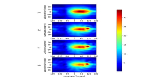
The ionospheric VTEC maps of CNES, RRTGIM-1, RRTGIM-3, and RRTGIM-6 at 12:00 UT, DOY 78, 2020, are shown in Figure 5. For the four subfigures, (a) is the ionospheric VTEC map of CNES, while (b), (c), and (d) are the ionospheric VTEC maps of RRTGIM-1, RRTGIM-3, and RRTGIM-6, respectively. As we can see, all models showed similar diurnal and geographic features. Maps of the three refined models showed more details compared to the CNES VTEC map, especially for the region around 110° E, 20° N, where the refinement GNSS stations were located. Three refined models showed a very similar distribution. The difference maps of RRTGIMs to CNES are shown in Figure 6. For the three subfigures, (a), (b), and (c) were RRTGIM-1, RRTGIM-3, and RRTGIM-6, respectively. As shown in the figure, the bias values were minimal for most areas except for the region around 110° E, 20° N. For the three models, the bias ranged from −2.5 to 8.3 TECU. The most considerable bias was around the refinement stations. The largest and smallest bias of three RRTGIM models were 10.47, 10.54, 13.14 TECU, and −3.50, −2.56, −4.13 TECU, respectively. The result showed the influence was mainly limited to the region around the refinement GNSS stations.

The modeling procedure is referred to in Figure 4. Post-residual errors of refinement modeling were used to assess internal coincidence accuracy. Histograms of residual errors in a 1 h interval are shown in Figure 7, Figure 8 and Figure 9. The root mean square (RMS) and mean values are calculated as well. The maximum RMS of the three models was 2.39, 2.43, and 1.99 TECU, where the minimum RMS was 0.76, 0.29, and 0.89 TECU. The average residual errors of the three models ranged 0.03–0.86 TECU, 0.08–0.75 TECU, and 0.01–0.42 TECU for the whole day. The internal coincidence accuracy of the three models was very high, according to the residual error values.

Refinement tests from DOY 78 to 99, 2020, were carried out to further investigate refinement modeling. The average bias and RMS of post-residuals are shown in Figure 10. The average RMS of RRTGIM-1 was 1.04 TECU, which was smaller than the 1.28 TECU of RRTGIM-3 and 1.29 TECU of RRTGIM-6, showing that the model with fewer stations had better internal coincidence accuracy. The average bias of the three models was −0.15, −0.03, and −0.01 TECU, showing that RRTGIM-6 was more stable than RRTGIM-3 or RRTGIM-1.

4.2. Comparison with STEC Derived from the GNSS Dual-Frequency Measurement

STEC calculated from RRTGIM products was evaluated to denote model accuracy. Real-time VTEC product of CNES and post-process VTEC product of CODE were also evaluated in the comparison. By comparing the difference between these products and STEC derived from the GNSS dual-frequency measurement, the accuracy of the five products was evaluated.

First, we conducted an STEC comparison of 12 stations in China. RMSE values of different ionospheric VTEC models are shown in Figure 11. The maximum RMSE was 8.37 TECU for B027, the minimum RMSE was 2.83 TECU for BJFS, and the average RMSE of CNES was 5.73 TECU. Compared with CNES, RRTGIM-1 had better performance. The average RMSE of RRTGIM-1 was 3.55 TECU, which was smaller than CNES. For B005, B027, B081, HKKT, and HKNP, the improvement was 3.88, 3.87, 3.34, 3.93, and 3.92 TECU, which reached to 48%, 46.3%, 47.6%, 52.7%, and 52.7%, respectively. The average RMSE of RRTGIM-3 and RRTGIM-6 was 3.53 and 3.11 TECU, which was slightly better than RRTGIM-1. The CODE ionospheric VTEC product was the post-process ionospheric VTEC product that used for more than 300 global IGS stations. In general, CODE had a better performance than CNES. In this test, the average RMSE of CODE was 4.9 TECU, which was better than CNES. However, RRTGIM models had greater improvement than CNES, which was better than CODE. As the best refinement model, RRTGIM-6’s average RMSE was 3.11 TECU. The improvement was 45.7% and 36.5% for CNES and CODE, respectively.

Moreover, to evaluate the accuracy of ionospheric activity time, we conducted comparisons at UT 6:00 DOY 78, 2020. As shown in Figure 12, the average RMSE was 6.11 TECU for CNES, where the maximum was 10.45 TECU for HKNP and the minimum was 2.38 TECU for B019. RRTGIM-1 showed some improvement when compared with CNES. The maximum therein was 5.88 TECU for B016 and the minimum was 2.13 TECU for B019. Moreover, the average RMSE was 3.89 TECU, which was a 36.3% improvement over CNES. For the three refinement models, RRTGIM-6 had the best performance and the average RMSE was 3.41 TECU, which was a 44.1% improvement over CNES. The average RMSE of CODE was 4.6 TECU, which was better than CNES but worse than three refinement models. The improvement was 12.6%, 17.4%, and 25.9% for RRTGIM-1, RRTGIM-3, and RRTGIM-6, respectively.

To evaluate the ionospheric VTEC models further, we conducted a STEC assessment for DOY 78–99, 2020. Figure 13 illustrates the average and standard deviation (STD) of STEC RMSE values in the period. The average RMSE of all GNSS stations was 6.74 TECU for CNES. Further, the maximum was 9.67 TECU for B031 and the minimum was 3.11 TECU for BJFS. Meanwhile, the average RMSE of all stations for RRTGIM-1 was 3.62 TECU, where the maximum was 5.62 TECU for B031 and the minimum was 2.52 TECU for HKKT. RRTGIM-1 had a 46.3% improvement over CNES on average. Moreover, the average RMSE of all stations was 5.13 TECU for CODE. For all stations, RRTGIM-1 was better than CODE. The improvement to CODE was 29.4%. Although three stations were used for RRTGIM-3, the improvements to RRTGIM-1 were not obvious. Especially for some stations, RMSE was greater than RRTGIM-1. The average RMSE of all stations for RRTGIM-6 was 3.05 TECU, which was smaller than RRTGIM-1 and RRTGIM-3. The improvements to CNES and CODE were 40.5% and 54.7%, respectively.

To verify the influence of other regions, we adopted 12 globally distributed stations. RMSE was calculated for each station. As shown in Figure 14, the influence of other regions was very slight. For the 12 stations, the most apparent affected station was GMSD in Japan, where the RMSE was 3.39, 3.22, 2.86, and 2.79 TECU for CNES, RRTGIM-1, RRTGIM-3, and RRTGIM-6. The improvement to CNES was 17.7% for RRTGIM-6. For other stations, the RMSE was almost the same after refinement modeling.

Jason-3 VTEC products between DOY 78 and 99, 2020 in the region 97–127°E, 18–45°N were extracted as the reference. VTEC comparisons of three refinement models CNES and CODE were carried out. The latitudinal variation of RMSE of the refinement models CNES and CODE are shown in Figure 15. As shown in the figure, along with the rise of latitude, RMSE of the models became smaller. The RMSE ranged from 4.6 to 5.7 TECU. As a refined model of CNES, RRTGIM-1 had a better performance than CNES. The improvements to CNES ranged from 0.2 to 0.8 TECU for different latitudes. RRTGIM-3 had a slightly better performance than RRTGIM-1 for different latitudes. Meanwhile, the RMSE of RRTGIM-6 ranged from 3.3 to 4.3 TECU, showing the best performance in the five models.

The mean RMSE and bias of the 22 days are calculated and shown in

Table 5. Mean RMSE and mean bias of VTEC products (unit: TECU).

Product	CODE	CNES	RRTGIM-1	RRTGIM-3	RRTGIM-6
Mean RMSE	4.93	5.14	4.67	4.55	4.05
Mean bias	1.72	1.80	1.47	1.51	1.40

. As can be seen, the average RMSE of CNES was 5.14 TECU. The average RMSE values of three RRTGIM products were 4.67, 4.55, and 4.05 TECU, which were better than CNES. The improvement to CNES was 9.1%, 11.5%, and 21.2%. Moreover, CODE’s average RMSE was 4.93 TECU, which was worse than the refinement models.

4.3. Performance Analysis of Real-Time Single-Frequency PPP

RT-SF-PPP tests were carried out to evaluate the performance of the RRTGIM models, as well as CODE and CNES ionospheric VTEC products. RT-SF-PPP experiments with 12 GNSS stations in China were conducted. Orbit and clock corrections from CLK93 were adopted to correct orbit and clock errors. Tropospheric errors were corrected by the Saastamoninen model. Note that RT-SF-PPP was simulated by processing the GNSS data in the post mode. Detail processing strategies for the RT-SF-PPP solution are listed in

Table 6. Details processing strategies for the SF-PPP solution.

Option	Setting
Positioning mode	PPP Kinematic
Orbit	Broadcast+CLK93
Clock	Broadcast +CLK93
Frequencies	L1
Ionospheric correction	CODE/CNES/RRTGIM-1/RRTGIM-3/RRTGIM-6
Tropospheric correction	Saastamoinen model

.

Daily static PPP solution with IGS final product was adopted as the reference. Position errors of RT-SF-PPP are shown in Figure 16. As can be seen, positioning errors of the five ionospheric models on horizontal and vertical components reached submeter-level and meter-level. For CNES, the maximum and minimum error of stations on horizontal was B016 and B081, which were 1.04 and 0.91 m on the north component, and 0.25 and 0.29 m on the east component. For the up component, the maximum and minimum error was 2.69 m on station B081 and 0.61 m on station BJFS. For RRTGIM-1, the average RMSE values on the north, east, and up components were 0.45, 0.51, and 1.39 m. The improvement to CNES was 22.4%, 28.2%, and 24.9%. RRTGIM-3 and RRTGIM-6 had a slightly better performance than RRTGIM-1. The average RMSE values for RRTGIM-3 were 0.44, 0.49, and 1.39 m, and for RRTGIM-6 were 0.42, 0.46, and 1.32 m. The average CODE RMSE was 0.49, 0.62, and 1.56 m, which was better than CNES.

To investigate positioning accuracy using ionospheric models further, RT-SF-PPP was conducted from DOY 78 to 99, 2020. As shown in Figure 17, the average RMSE in 22 days was 0.56, 0.68, and 1.8 m for the three components. CODE performed better than CNES and the average RMSE was 0.53, 0.64, and 1.5 m. RRTGIM-1 also performed better than CNES and CODE, and the average RMSE was 0.46, 0.5, and 1.4 m for the three components. The improvements to CODE were 13.2%, 21.9%, and 7.9%, and for CNES were 17.9%, 26.5%, and 22.2%. Moreover, RRTGIM-3 and RRTGIM-6 were slightly better than RRTGIM-1. The average RMSE of RRTGIM-3 was 0.45, 0.50, and 1.4 m, and for RRTGIM-6 were 0.44, 0.46, and 1.34 m.

5. Discussion

Ionospheric delay is a crucial error in SF-PPP. Ionospheric VTEC products broadcasted with CNES RTS are a widely used RTGIM product. However, due to the uneven distribution of IGS GNSS stations, the accuracy of the CNES VTEC products is nonuniform. To generate an accuracy-consistent VTEC product for China, we proposed a real-time refinement method. Three refinement models: RRTGIM-1, RRTGIM-3, and RRTGIM-6, used one, three, and six GNSS stations. These models were built and evaluated in 22 days, from DOY 78 to 99, 2020. The performance evaluation was carried out in three parts: (1) residual error analysis of refinement modeling, (2) comparison with external ionospheric TEC data, and (3) performance analysis of RT-SF-PPP.

The modeling residual errors show that internal coincidence accuracy was very high. The average RMSE and bias were 1.04, 1.28, and 1.29 TECU, and −0.15, 0.03, −0.01 TECU for the three models. We determined that RRTGIM-6 had the best stability.

Two external TEC products were used as a reference to verify refinement model accuracy: STEC derived from dual-frequency measurement and VTEC derived from Jason-3. STEC accuracy from DOY 78 to 99, 2020, was assessed in support of 12 stations as a reference. The average RMSE was 6.74 TECU and the refinement models had better performance than CNES and CODE. The average RMSE of RRTGIM-1, RRTGIM-3, and RRTGIM-6 were 3.62, 3.55, and 3.05 TECU, respectively. Meanwhile, the influence of refinement was very limited in other regions. All stations had few influences after refinement. For Jason-3 VTEC product comparison, data points in the region 97–127° E, 18–45° N were compared from DOY 78 to 99, 2020. The average RMSE was 5.14 TECU for CNES. Meanwhile, the average RMSE values were 4.67, 4.55, and 4.05 TECU for the three refinement models. The improvement was 9.1%, 11.5%, and 21.2%, respectively. Although RRTGIM-1 was refined by only one station, it had an apparent improvement for CNES and CODE. Meanwhile, the other two refinement models also had better performance than CNES and CODE.

The positioning accuracy of RT-SF-PPP was assessed in support of ionospheric VTEC products. In total, 12 GNSS stations in China were used to carry out the RT-SF-PPP experiment. Results showed that RT-SF-PPP with CNES VTEC products achieved performance with 0.56, 0.68, and 1.8 m in the north, east, and up components. For CODE, the positioning accuracy was 0.53, 0.64, and 1.52 m in the three components. RRTGIM-1 had a better performance than CNES or CODE, and the RMSE values were 0.46, 0.50, and 1.4 m, which had 17.9%, 26.5%, and 22.2% improvement to CNES and 13.2%, 21.9%, and 7.9% improvement to CODE. The positioning accuracy of RRTGIM-6 was 0.44, 0.46, and 1.34 m, which had the highest performance of the three refinement models. Therefore, we concluded that the proposed refinement method was an effective method to refine CNES VTEC products. Even when using only one station in the refinement method, we achieved a better performance compared to CODE ionospheric products in China. Moreover, RRTGIM-6 had the best performance out of the three refinement models.

As te improvement is noticeable, the refinement method proposed in this study is significant. To model more accurate ionospheric VTEC, a feasible alternative is in using more GNSS stations. However, the quantity of publicly accessed GNSS stations, like the IGS network, is small. Furthermore, there are thousands of GNSS stations across the world, but access is limited. Based on the real-time VTEC model and local GNSS stations, the administrative department of a GNSS station can easily build higher accuracy and representation consistency into the VTEC product. Meanwhile, for low accuracy regions, one can conveniently build new GNSS stations to improve the region’s accuracy.

6. Conclusion

Because the accuracy of the real-time global VTEC products (like CNES VTEC product) is nonuniform, we proposed a refinement method of a real-time ionospheric VTEC model for China and carried out experiments to validate the model effectiveness. The results show that the proposed method was an effective method to refine real-time VTEC products. Based on the real-time VTEC model and local GNSS stations, one can conveniently easily build higher accuracy and representation consistency into the VTEC product.

References

- Zumberge, J.F.; Heflin, M.B.; Jefferson, D.C.; Watkins, M.M.; Webb, F.H. Precise Point Positioning for the efficient and robust analysis of GPS data from large networks. J. Geophys. Res. Solid Earth 1997, 102, 5005–5017. [Google Scholar] [CrossRef] [Green Version]
- Kouba, J.; Springer, T. New IGS station and satellite clock combination. GPS Solut. 2001, 4, 31–36. [Google Scholar] [CrossRef]
- Bisnath, S.; Gao, Y. Current State of Precise Point Positioning and Future Prospects and Limitations. In Observing our Changing Earth; Springer Berlin/Heidelberg: Berlin/Heidelberg, Germany, 2009; pp. 615–623. [Google Scholar]
- Yang, H.; Lan, H.; Liu, F.; Gao, Y.; Elsheimy, N. IP3/DR-A low-cost precise and robust GNSS/INS integrated navigation system for land vehicles. In Proceedings of the 2020 IEEE 91st Vehicular Technology Conference (VTC2020-Spring), Antwerp, Belgium, 25–28 May 2020; pp. 1–5. [Google Scholar]
- Teunissen, P.J.G.; Jonkman, N.F.; Joosten, P.; Tiberius, C.C.J.M. Long baseline 3 frequency differential GNSS. In Proceedings of the IEEE 2000. Position Location and Navigation Symposium (Cat. No.00CH37062), San Diego, CA, USA, 13–16 March 2000; pp. 7–14. [Google Scholar]
- Li, Y. A novel ambiguity search algorithm for high accuracy differential GNSS relative positioning. Aerosp. Sci. Technol. 2018, 78, 418–426. [Google Scholar] [CrossRef]
- Rizos, C.; Janssen, V.; Roberts, C.; Grinter, T. Precise Point Positioning: Is the era of differential GNSS positioning drawing to an end. In Proceedings of the FIG Working Week 2012, Rome, Italy, 6–10 May 2012; pp. 1–17. [Google Scholar]
- Zhang, L.; Yang, H.; Gao, Y.; Yao, Y.; Xu, C. Evaluation and analysis of real-time precise orbits and clocks products from different IGS analysis centers. Adv. Sp. Res. 2018, 61, 2942–2954. [Google Scholar] [CrossRef]
- Ge, M.; Gendt, G.; Rothacher, M.; Shi, C.; Liu, J. Resolution of GPS carrier-phase ambiguities in Precise Point Positioning (PPP) with daily observations. J. Geod. 2008, 82, 389–399. [Google Scholar] [CrossRef]
- Nie, Z.; Yang, H.; Zhou, P.; Gao, Y.; Wang, Z. Quality assessment of CNES real-time ionospheric products. GPS Solut. 2019, 23, 11. [Google Scholar] [CrossRef]
- Ren, X.; Chen, J.; Li, X.; Zhang, X.; Freeshah, M. Performance evaluation of real-time global ionospheric maps provided by different IGS analysis centers. GPS Solut. 2019, 23, 113. [Google Scholar] [CrossRef]
- Hadas, T.; Bosy, J. IGS RTS precise orbits and clocks verification and quality degradation over time. GPS Solut. 2014, 19, 93–105. [Google Scholar] [CrossRef] [Green Version]
- Kazmierski, K.; Sośnica, K.; Hadas, T. Quality assessment of multi-GNSS orbits and clocks for real-time precise point positioning. GPS Solut. 2017, 22, 11. [Google Scholar] [CrossRef] [Green Version]
- Zhang, L.; Yao, Y.; Peng, W.; Shan, L.; He, Y.; Kong, J. Real-Time Global Ionospheric Map and Its Application in Single-Frequency Positioning. Sensors 2019, 19, 1138. [Google Scholar] [CrossRef] [PubMed] [Green Version]
- Li, Z.; Wang, N.; Hernández-Pajares, M.; Yuan, Y.; Krankowski, A.; Liu, A.; Zha, J.; García-Rigo, A.; Roma-Dollase, D.; Yang, H.; et al. IGS real-time service for global ionospheric total electron content modeling. J. Geod. 2020, 94, 32. [Google Scholar] [CrossRef]
- Fujita, S.; Yamamoto, H.; Iura, T.; Kubo, Y.; Sugimoto, S. Modeling ionosphere VTEC over Japan based on GNSS regression models and GEONET. Int. J. Innov. Comput. Inf. Control 2010, 6, 155–169. [Google Scholar] [CrossRef] [Green Version]
- Banville, S.; Collins, P.; Zhang, W.; Langley, R.B. Global and Regional Ionospheric Corrections for Faster PPP Convergence. Navigation 2014, 61, 115–124. [Google Scholar] [CrossRef]
- Tu, R.; Zhang, H.; Ge, M.; Huang, G. A real-time ionospheric model based on GNSS Precise Point Positioning. Adv. Space Res. 2013, 52, 1125–1134. [Google Scholar] [CrossRef]
- Aggrey, J. Assessment of global and regional ionospheric corrections in multi-GNSS PPP. In Proceedings of the 31st International Technical Meeting of The Satellite Division of the Institute of Navigation (ION GNSS+ 2018), Miami, FL, USA, 24–28 September 2018; pp. 24–28. [Google Scholar]
- Zhang, B. Three methods to retrieve slant total electron content measurements from ground-based GPS receivers and performance assessment. Radio Sci. 2016, 51, 972–988. [Google Scholar] [CrossRef] [Green Version]
- Jee, G.; Lee, H.-B.; Kim, Y.H.; Chung, J.-K.; Cho, J. Assessment of GPS global ionosphere maps (GIM) by comparison between CODE GIM and TOPEX/Jason TEC data: Ionospheric perspective. J. Geophys. Res. Space Phys. 2010, 115. [Google Scholar] [CrossRef] [Green Version]
- Li, M.; Yuan, Y.; Wang, N.; Li, Z.; Huo, X. Performance of various predicted GNSS global ionospheric maps relative to GPS and JASON TEC data. GPS Solut. 2018, 22, 55. [Google Scholar] [CrossRef]
- Jin, R.; Jin, S.; Feng, G. M_DCB: Matlab code for estimating GNSS satellite and receiver differential code biases. GPS Solut. 2012, 16, 541–548. [Google Scholar] [CrossRef]
- Liu, T.; Zhang, B.; Yuan, Y.; Li, M. Real-Time Precise Point Positioning (RTPPP) with raw observations and its application in real-time regional ionospheric VTEC modeling. J. Geod. 2018. [Google Scholar] [CrossRef]
- Blewitt, G. An automatic editing algorithm for GPS data. Geophys. Res. Lett. 1990, 17, 199–202. [Google Scholar] [CrossRef] [Green Version]
Publisher’s Note: MDPI stays neutral with regard to jurisdictional claims in published maps and institutional affiliations. |
Figure 1.
Distribution of GNSS stations for refinement modeling.
Figure 2.
Global distribution of 24 validation stations: (a) distribution of 12 GNSS stations in China and (b) distribution of 12 IGS GNSS stations across the world.
Figure 3.
The difference to CODE (Center for Orbit Determination in Europe) in cycle 152: (a) ascending passes and (b) descending passes.
Figure 4.
The procedure of refinement modeling.
Figure 5.
Ionospheric VTEC map (UT 12:00, DOY 78, 2020) of CNES (a), RRTGIM-1 (b), RRTGIM-3 (c), and RRTGIM-6 (d).
Figure 6.
Differences between RRTGIM-1 (a), RRTGIM-3 (b), and RRTGIM-6 (c) and CNES.
Figure 7.
Post-residual distribution of refinement modeling in DOY 78 of RRTGIM-1.
Figure 8.
Post-residual distribution of refinement modeling in DOY 78 of RRTGIM-3.
Figure 9.
Post-residuals distribution of refinement modeling in DOY 78 of RRTGIM-6.
Figure 10.
Root mean square (RMS) of modeling VTEC residuals from DOY 78 to 99, 2020, of RRTGIM-1, RRTGIM-3, and RRTGIM-6.
Figure 11.
Slant total electron content (STEC) RMSE of CODE, CNES, and RRTGIMs on DOY 78, 2020.
Figure 12.
STEC RMSE of CODE, CNES, and RRTGIMs at UT 6:00, DOY 78, 2020.
Figure 13.
The average and standard deviation (STD) of STEC RMSE for 12 GNSS stations in China for DOY 78–99, 2020.
Figure 14.
STEC RMSE of the 12 global stations on DOY 78,2 April 2020 Comparison with VTEC derived from Jason-3.
Figure 15.
Latitudinal variation of RMSE errors of the VTEC products.
Figure 16.
Positioning accuracy of SF-PPP using five products on DOY 78, 2020.
Figure 17.
Positioning accuracy over 22 days for SF-PPP using VTEC products.