Article

Identification of Mung Bean in a Smallholder Farming Setting of Coastal South Asia Using Manned Aircraft Photography and Sentinel-2 Images

1
CIMMYT-Bangladesh, House 10/B. Road 53, Gulshan-2, Dhaka 1213, Bangladesh
2
CIMMYT-Henan Collaborative Innovation Center, Henan Agricultural University, Zhengzhou 450002, China
*
Author to whom correspondence should be addressed.
Remote Sens. 2020, 12(22), 3688; https://doi.org/10.3390/rs12223688
Submission received: 1 October 2020 / Revised: 27 October 2020 / Accepted: 3 November 2020 / Published: 10 November 2020

Abstract

:
Mung bean (Vigna radiata) plays an important role providing protein in the rice-based diet of the people in Bangladesh. In the coastal division of Barisal, our study area, the average farm size is less than 0.5 ha and individual fields measure about 0.10 ha. The availability of free Sentinel-2 optical satellite data acquired at a 10 m ground sampling distance (GSD) may offer an opportunity to generate crop area estimates in smallholder farming settings in South Asia. We combined different sources of in situ data, such as aerial photographs taken from a low flying manned aircraft, data collected on the ground, and data derived from satellite images to create a data set for a segment based classification of mung bean. User’s accuracy for mung bean was 0.98 and producer’s accuracy was 0.99. Hence, the accuracy metrics indicate that the random tree classifier was able to identify mung bean based on 10 m GSD data, despite the small size of individual fields. We estimated the mung bean area for 2019 at 109,416 ha, which is about 40% lower than the Department of Agricultural Extension estimates (183,480 ha), but more than four times higher than the 2019 data reported by the Bangladesh Bureau of Statistics (26,612 ha). Further analysis revealed that crop production tends to be clustered in the landscape by crop type. After merging adjacent segments by crop type, the following average cluster sizes resulted: 1.62 ha for mung bean, 0.74 ha for rice (Oryza sativa), 0.68 ha for weedy fallow and 0.40 ha for a category of other crops. This explains why 10 m GSD satellite data can be used for the identification of predominant crops grown in specific regions of South Asia.

Graphical Abstract

1. Introduction

Remote sensing can play an important role in monitoring indicators of agricultural production, poverty, and malnutrition in consideration of the Sustainable Development Goals (SDG) 2030 agenda [1]. Geographic knowledge of where and how much of a crop is grown is crucial for productivity that is prerequisite to food security, in terms of diversity of food supply and potential production in the face of disasters. It can also provide a base line to measure the impact of development initiatives and investments over time as farmers grow successive crops [2]. Cropped area estimates are also key for national agricultural monitoring and statistical reporting, in addition to technology targeting in development programs [3].
Barisal division of Bangladesh, located in the coastal Ganges-Brahmaputra delta, is home to more than eight million people and measures 1,364,500 ha. Close to 40% of the region’s children are affected by malnutrition and stunting [4]. Mung bean (Vigna radiata) is grown during the dry winter months within this region, both as a market oriented cash crop and for home consumption. Mung bean helps diversify and add protein to the predominantly rice based diet of smallholder farmers in the coastal region [5,6,7]. It is usually grown as a broadcast ‘opportunity’ crop without intensive management or inputs other than seed. As a species, it is however somewhat salinity and drought tolerant—traits of key interest in the climate extreme prone coastal area [8,9]. Although growing in acreage, specific production estimates for cropped mung bean area vary greatly. According to the 2019 data published by the Bangladesh Bureau of Statistics (BBS) [10], total mung bean area was just 26,612 ha. However, according to data obtained from Bangladesh’s Department of Agricultural Extension, cropped mung bean area was nearly seven times greater, at about 183,480 ha in 2019. These discrepancies are important, and represent differences in data collection methodologies, which can affect agricultural policy planner decisions and investments in rural development initiatives.
The agricultural landscape in Barisal Division is similar to other regions in South Asia that rotate winter season crops with monsoon season paddy rice production. They are densely populated and farmers cultivate every square meter of land. Due to the tradition of splitting up the land among the male children of the farm family, average farm size is about 0.3 ha and individual parcel sizes measure 0.08 ha for small and 0.16 ha for medium farms [11]. In a study on field boundary delineation conducted in Barisal division, [12] reported an average parcel size of 0.10 ha. Fields are separated by bunds, usually about 0.25 m wide. Many fields can also generally only be accessed by foot. Coastal Bangladesh is mostly flat and less than 3 m above sea level. The southern half of the division is protected by polders, which are coastal embankments meant to protect villages and agricultural fields against oceanic water intrusion and salinization [13]. Most of the land is however tidally flooded during the monsoon season, as polder walls are in widespread disrepair. Flooding depth and duration limit crop choices that can be grown during the winter months, as farmers have to wait for rice harvest after the end of the monsoon rains until the fields are sufficiently drained to establish a subsequent winter season crop. Premonsoon rainstorms that may begin as early as March determine the end of the period during which non-rice crops can be cultivated in the winter. Estimates are that about 14% of the cropland of Barisal Division remains fallow during the winter months, mostly due to salinity in the coastal zone [14,15].
Road infrastructure in this region is also poor [16], with many roads being too narrow for regular vehicles. As such, most smallholders’ parcels can be accessed only by foot. This makes ‘windshield’ surveys challenging; in addition, in situ data collection is time consuming. Considering these issues, BBS uses two approaches to assess the extent of agricultural land under different crops [10]. The first is based on direct observation of crops in the field, though this approach is applied only to major crops, such as rice, wheat, potato and jute. For minor crops, such as mung bean, lentils (Lens culinaris) or grass pea (Lathyrus sativus L.) BBS conversely relies on household surveys. In each union, the smallest administrative district, which typically measures 3200 ha, enumerators interview five farmers. Resulting data are then aggregated to the next higher administrative unit, using data from the previous or a normal year and their local expertise. Data are then reported at the district level.
Satellite-based remote sensing has been proposed as a viable alternative for agricultural land use and crop monitoring [17]. The availability of free satellite data and automated image preprocessing toolboxes for atmospheric correction and cloud detection, such as SNAP [18], has opened new opportunities for using time series of images for crop classification. The advantages of using time series of optical imagery for land cover classification were described in a review by [19]. In an example from the Canadian Prairies, [20] showed how classification accuracy increases with the number of images used over a cropping season, when classifying crops at the field level. They also compared various machine learning algorithms, such as random forest (RF) [21], artificial neural networks (ANN) [22,23] and support vector machine (SVM) analyses [24] to the maximum likelihood algorithm. All machine learning algorithms performed better than the maximum likelihood algorithm, and differences in overall accuracies obtained with the machine learning algorithms became negligible with an increasing number of images used for the classification. Speed and ease of use are additional factors to be considered when choosing a classifier. In a review of the RF classifier, [25] concluded that it requires the setting of fewer parameters and also performs faster than other classifiers.
In Bangladesh, and especially in the coastal region, few remote sensing studies on crop identification have been carried out. They mainly focused on fallow land identification or the distinction between crop and pasture land [26]. In order to identify cropland categories including (i) fallow land, (ii) low management intensity crops (primarily consisting of pulse crops) and (iii) and high management intensity crops (such as wheat, boro rice, maize and mustard), [15,27] analyzed Landsat 5, 7 and 8 satellite images to train a RF classifier. Classification was based on an object-based image analysis (OBIA) segmentation and used four input layers including the (i) mean of the digital numbers of bands, (ii) texture (all direction), (iii) NDVI and (iv) the ratio of the NIR and visible bands. In another study, OBIA segmentation of a RapidEye satellite image with a ground sampling distance (GSD) of 5 m was used to train an RF algorithm to identify maize fields for a yield gap analysis in Northern Bangladesh [28]. However, most crop identification studies in Bangladesh have focused on rice. While the size of individual rice paddies are small, it is grown in large contiguous areas and can therefore be identified with MODIS [29], Landsat [30] or microwave [31]. In neighboring India, multi-date AWiFS data were used to identify pulse crops [32]. In areas with contiguous acreage devoted to legumes, they reached an accuracy of more than 95%, whereas in regions with scattered pulse fields, which are analogous to the smallholder farming conditions of Southern Bangladesh, accuracies dropped to 50–81%. As to our knowledge, no previous research has been conducted on identifying mung bean or any other minor crop using satellite data for coastal Bangladesh.
Our analysis focuses on the use of images collected with the Sentinel-2A and -2B satellites that are freely available and have a GSD of 10 m. Since March of 2017, these satellites have covered the globe at an interval of five days, thus opening up the opportunity to test the applicability of a time-series approach based on Sentinel-2 data for crop classification in smallholder farmer settings, where fields are smaller than in most other parts of the world. There is uncertainty regarding the accuracy of official mung bean area estimates and remote sensing might provide a cost effective tool to improve crop area estimates in Bangladesh, especially for the pulse crops that are grown during the rather cloud free winter months. This paper responds to this opportunity and aims to (a) demonstrate a method that integrates multi-source in situ data for crop identification in a region where access to fields is challenging and time consuming and (b) to test the suitability of a multi-temporal, segmentation based classification algorithm to identify mung bean with remotely sensed data.

2. Materials and Methods
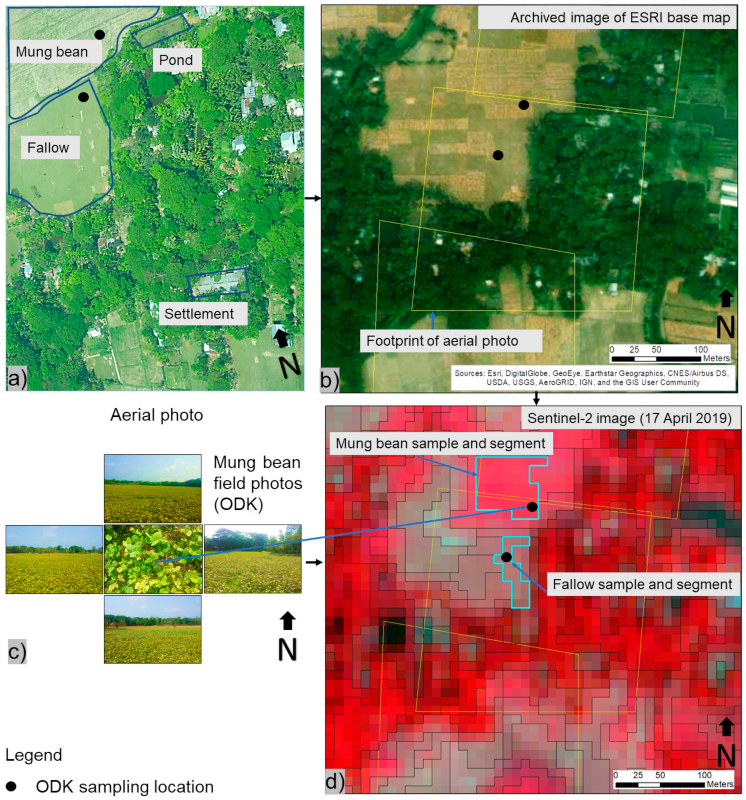
2.1. Study Area

This study focuses on Barisal, one of eight administrative divisions of Bangladesh, which measures 1,364,500 ha, with a cropland area of 543,000 ha [15]. The division is divided into six districts named Barguna, Barisal, Bhola, Jhalokati, Patuakhali and Pirojpur (Figure 1). During the rainy season from June to November, most of the land is flooded and used for rice production. After rice harvest in November and December, farmers grow grass pea (Lathyrus sativus), which is typically seeded into the rice crop before harvest, lentil (Lens culinaris) and mung bean. In some areas, farmers may also grow winter boro rice starting in February, but on limited land areas [15]. Grass pea reaches maturity in February; after harvest, land is left fallow and the weeds take over. These fields are then typically used for opportunistic grazing until they become inundated by monsoon rains starting in late April. For this analysis, we did not distinguish between the land that is left fallow during the entire winter rabi season or after grass pea harvest. For mung bean identification, we are focusing on the period from February to April. We therefore consider all land not cultivated during this period as weedy fallow.
Mung bean is typically sown in early February and grown without irrigation. To preserve soil moisture for germination, farmers till the soil and plant on the same day. However, early growth may be aided by occasional rains. Once established, mung bean mostly draws from the shallow (1–2 m depth) water table for evapotranspiration during its growth period [33]. Harvest starts in late March and continues through early May. Mung bean is an indeterminate crop and farmers will pick pods 2–3 times until senescence [34].

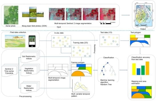
2.2. Analysis Framework

We combined four sources of data in order to prepare the training and test data (Figure 2), including (i) aerial photographs taken from a low flying aircraft, (ii) data collected on the ground, based on selected photos from the aerial campaign, (iii) data derived from visual inspection of Google Earth (Google, Mountain View, San Francisco, CA, United States) and ArcGIS (Version 10.7.1, Environmental Systems Research Institute (ESRI), Redlands, CA, United States) World Imagery and (iv) Sentinel-2 imagery. The data points with information on land use and crop type were linked to the attribute table of Sentinel-2 derived segments. The resulting data set was split into two groups including 66.6% of each class for training and the remainder for testing.

2.3. Satellite Image Preprocessing

All available Sentinel-2 images with less than 10% cloud cover acquired between February 6 and April 17 of 2019 were downloaded from the European Space Agency’s (ESA) Sentinel Scientific Data Hub. We used the Sen2Cor atmospheric correction processor version 2.5.5 [35] of the Sentinel Application Platform SNAP v7.0 distributed under the GNU general public license to calculate bottom-of-atmosphere (BOA) reflectance. Given the small field sizes, we used only the four 10 m bands B2 (490 nm), B3 (560 nm), B4 (665 nm) and B8 (842 nm) of Sentinel-2 for all subsequent analyses, including the segmentation. Barisal division is almost fully covered by these two Sentinel tiles: T45QZE and T45QZF. The 90° east meridian runs across our study area. The Sentinel-2 images in the UTM WGS84, zone 45 N projection provided a better coverage than those in zone 46. We therefore used the former as a base for all analyses. In order to cover the entire mung bean growing season from February to the end of April, images from February 6, March 8 and March 28 were selected (Figure 3). Visual inspection, and the meta-data, revealed that they were cloud free. However, all April images had some cloud cover. We used the images acquired on April 7, 17 and 22 to create a composite image, applying a median filter to generate cloud free pixels [36]. We subsequently did a visual check of the composite image and masked an area of 4397 ha area as cloudy. The image in early February covered the sowing period. Mung bean reached canopy closure in late March and harvest starts in April. Most mung bean varieties grown in Bangladesh are indeterminate, thus farmers can pick mung bean 2–3 times until early May, depending on the pest, rainfall and waterlogging conditions.
We used the Sentinel Application Platform (SNAP) to calculate the nine indices shown in Table 1. The resulting data layers were mosaicked and clipped to the boundaries of Barisal division using ArcGIS. The indices were developed to identify different water, soil and vegetation conditions. We needed to separate water bodies from the cropland and the paddy rice from the other crops. We relied on the normalized difference water index (NDWI) and the second normalized difference water index (NDWI2) for this task. Farmers generally till the soil before sowing mung bean in order to control the weeds and to prepare a seed bed. This results in bright and bare soil conditions, which can be captured with the brightness index (BI) and the second brightness index (BI2), and the color index (Cl). We relied on four types of vegetation indices in order to characterize the canopies of the crops: the normalized difference vegetation (NDVI), enhanced vegetation index (EVI), green normalized difference vegetation index (GNDVI) and the soil adjusted vegetation index (SAVI).

2.4. Segmentation of Multi-Temporal Images
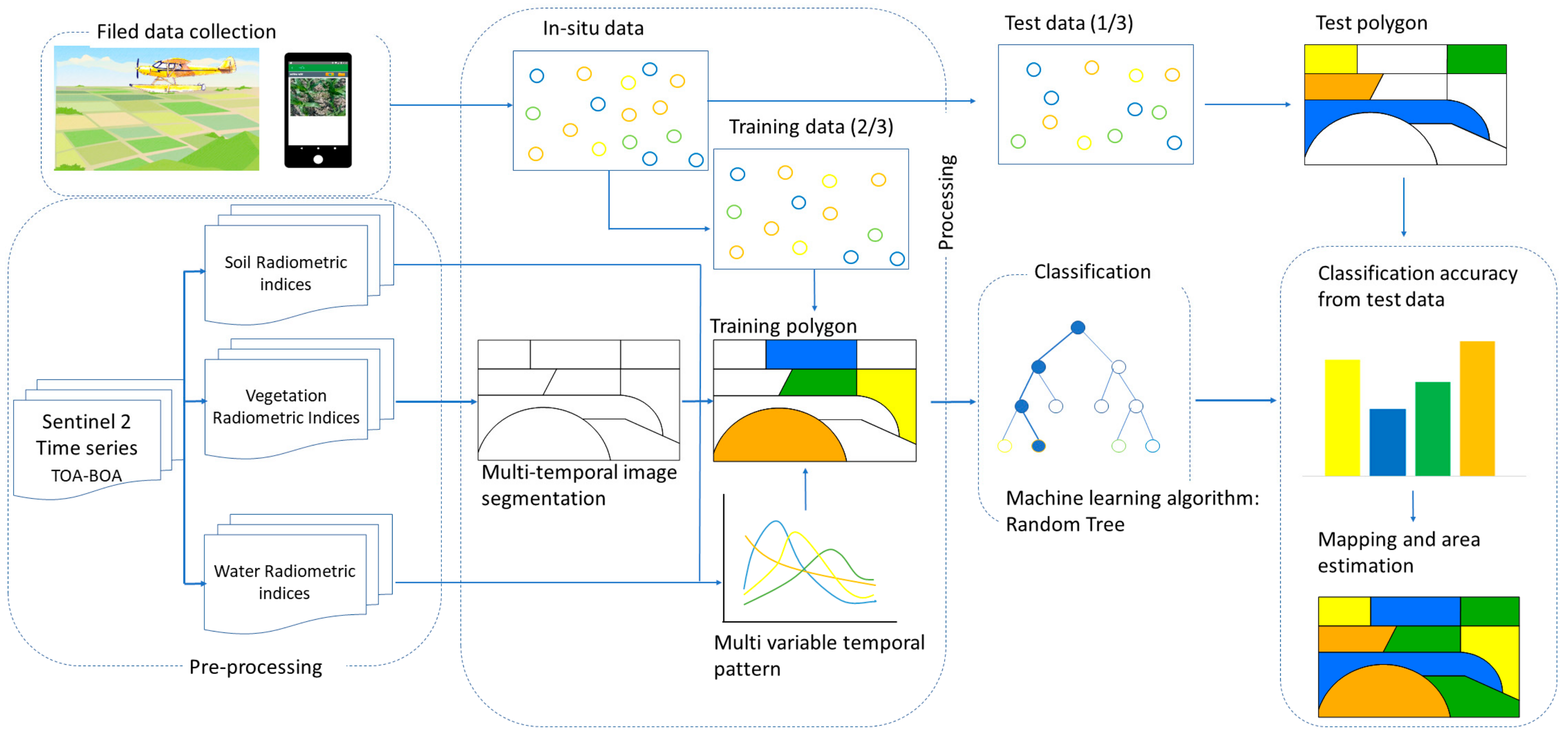
Initial analyses showed that the major challenge was to distinguish weedy fallow land from mung bean. These two species dominate the cropland area. Weedy fallow often succeeds grass pea and is grazed frequently. In order to create segments that separate the two types, we used a total of five layers including the time series of NDVI layers of the four images and EVI from the cloud free April mosaic. EVI has previously been used to successfully separate low input crops from fallow land in this region [15,27]. We used eCognition Developer (V9.5.1, Trimble Geospatial, Sunnyvale, CA, USA) to create the segments with the multi-resolution segmentation algorithm [45]. This region growing algorithm starts from the pixel level and iteratively aggregates pixels successively into objects until a condition of homogeneity set by the user is met. Based on visual inspection, a scale parameter of 0.5 created segments that best represented mung bean fields. Size and homogeneity were set to zero. Changing these two parameters had little effect on the shape of the segments, presumably because we used the data layers in float format and the segments were rather small. The weight for each of the four NDVI and the EVI layers was set to 1.

2.5. In Situ Data

2.5.1. Aerial Photos

Given the challenges of collecting representative in situ data in the Barisal division due to the poor road network, we made use of a manned, low-elevation aircraft to survey Barisal division for mung bean production. In order to cover the entire study area, we predefined a flight route of 410 km to be covered with a S2-AEC sea plane (Figure 4). Starting from Dhaka airport at 9:38 am on 25 March 2019, the flight took 2.25 h to complete at altitudes of 150–300 m above ground. The operator did not have the permission from the Bangladesh Civil Aviation Authority to mount a camera outside the aircraft. Hence, six passengers acquired photos with 2 Sony Nex-7, a Nikon DSLR, and a Canon 600D camera. We also used an iPhone and a Huawei Honor 8 smart phone. All images were acquired at the respective maximum resolutions: 6000 pixels × 4000 pixels for the Sony Nex-7 and Nikon DSLR, 5184 pixels × 3456 pixels for the Canon 600D, 4032 × 3024 for the iPhone 7 plus and 3968 × 2976 for the Xiaomi phone. Camera focus was set to infinity.
The flight track was recorded with a Bad Elf GNSS Surveyor GPS. In total, 3123 photos were taken, out of which 1917 were tagged to Sentinel-2 images. The footprints of the photos were manually digitized using the Sentinel-2 images and World Imagery in ArcGIS as a backdrop.

2.5.2. Ground Data Collection

In order to gather sufficient insights to interpret the aerial photos and determine the correct crop type that is visible in corresponding satellite images, we selected seven sampling areas along a transect. Two experienced field technicians spent a combined total of 20 days identifying the major crop types visible in preselected aerially acquired images. At each sampling point, located in the center of a crop field, they took one photo in each of the cardinal directions and a close-up photo of the crop with photo meta-data entered into tablets loaded with Open Data Kit (ODK) [46]. Data were retrieved from 537 sampling points, out of which 246 were used after conducting a plausibility check using Sentinel-2 data and Google Earth and World Imagery in ArcGIS. Photos from extremely small fields, which we could not discern from Sentinel-2 images, or that had GPS errors, or were located close to settlement areas with obscuring tree cover, were discarded. These GPS errors resulted from the proximity of trees and poor connections to cell phone tower networks. In a last step, the 246 data points were linked to the respective segments that encompassed them.

2.5.3. Visual Interpretation of Sentinel-2 Imagery

The 246 data points enabled the visual identification of additional points along the flight transect, using RGB and false color satellite images, and vegetation indices derived from Sentinel-2 images. False color satellite images, using the NIR, red and green bands were especially useful for the visual identification of mung bean, which had a distinct, dark pink color. For each patch or group of crop fields that were grown with the same crop types, we visually determined the center of the area and then assigned the crop to the segment encompassing it (Figure 5).

2.5.4. Google Earth and World Imagery

Barisal division is covered by Google Earth and ArcGIS World Imagery with high resolution images. However, most available images were not from the 2019 winter season and could not be used to identify crops. They could however be used to identify non-cropland, consisting of permanent features such as water bodies, roads, settlements and brick fields. In addition, we relied on Google Earth, Sentinel-2 images and local expert knowledge to identify rice fields on Bhola island, as it could not be included in our flight trajectory. We were able to identify paddy rice fields with the aid of Google Earth and false color Sentinel-2 images. When tagging the segments, we included all predominant non-land uses, such as roads, houses, trees and surface water bodies.
The above-mentioned sources of information were used to create training and validation data to distinguish cropland from non-cropland and in a subsequent step, to identity the crops grown on cropland. We used the following crop classes: (i) mung bean, (ii) weedy fallow, (iii) rice and (iv) other crops, consisting of wheat, maize, jute, lentil, soybean and vegetables. We did not identify grass pea, another crop widely grown in the study area during the winter months, as it had reached maturity in late February to mid-March and hence was outside of our aerial image acquisition period. In total, we tagged 2034 non-crop and 2358 segments with crop type information (Table 2). Mung bean and fallow land were represented by 900 segments each, whereas rice was represented by 441 and other crops by 72.

2.6. Quality Control of Crop Type Training Data

In order to check the consistency of the tagged crop type segments, we plotted their NDVI development over time (Figure 6). Among the four crop types, mung bean, typically sown in early February, had the lowest NDVI values on February 6 and on March 8. Its initial development, especially in comparison to the transplanted paddy rice, and to the weedy fallow, was relatively slow. In March, its canopy growth accelerated and kept developing at least until mid-April. Rice, in contrast, peaked in late March and started to senesce in early April. The other crops class consisted of lentil, wheat, maize, soybean and jute. The first four were planted before the end of the calendar year, after the completion of the monsoon season rice harvest and reached maturity in March and April. Jute, however, was sown in March only. On average, the NDVI values of these crops remained almost steady over time, but were always greater than those of weedy fallow, which was grazed during the winter months. The slight increase of the NDVI observed with weedy fallow in March can be attributed to weed growth following the onset of early rainfall during that month. The separation in NDVI between the weedy fallow and mung bean segments of the March 8 image indicates that our in situ data clearly distinguished between the two crops.

2.7. Identification of Cropland and Mung Bean

For the cropland and non-cropland and the subsequent mung bean identification, the respective data categories were split into training and test groups at a ratio of 2:1. We conducted the mung bean classification in two steps. We first identified cropland and subsequently the crop types within cropland. For the non-cropland vs. cropland identification, we used 1356 non-crop and another 1542 segments with crop type information, i.e., all training segments that were subsequently used for the identification of the crops grown on cropland.
We used the random tree (RT) classifier [47], which is built into eCognition for the classification. RT is a RF classifier. eCognition uses the former abbreviation and term, and for this reason we made use of the name RT in this paper. We maintained the same settings for the cropland vs. non-cropland and the subsequent crop identification. The depth of the random tree classifier was set to six and minimum sample count to five. The maximum number of categories was set to 16, and the maximum tree number to 50, with a forest accuracy of 0.01. All nine indices listed in Table 1 were used from each of the four image acquisition dates, resulting in 36 input layers.
There was a small region in the south of the study area, which had cloud cover even after applying a median filter to all three April images. For this 4397 ha area, we conducted a separate analysis, using the February 8 and the March 8 and 28 images. Results from these classifications were however not further discussed since the area located at the southern tip of Barisal division was negligible in size and nearly no mung bean was grown there due to excessively high soil salinity. The results were however applied to the completion of the crop type map and the area estimates.

2.8. Classification Accuracy Assessment

Classification accuracy was evaluated in terms of overall accuracy, user’s and producer’s accuracy [48], in addition to the Kappa Index of Agreement [49]. All accuracy related results are based on the test data, i.e., on the randomly selected one-third of the data that had been set aside before we started algorithm training. We also compared the resulting mung bean area estimates at the district level to statistics published by BBS [10] and data we had received from the DAE offices. DAE data were not published and used for internal purposes only.

2.9. Classification Scenarios

In order to answer questions as to how early and accurately mung bean cropland can be identified, we ran the following four scenarios, using different sequences of images: (1) February 6 image, (2) February 6 and March 8 images, (3) February 6, March 8 and 28 images and (4) all four images between February 6 and mid-April. Scenario 1 would be equivalent to an estimation of the area planted, whereas scenario 4 would represent an area harvested estimation. However, there was a caveat for the area planted estimation: we collected our in situ data in late March and early April only. A proper assessment of the feasibility to estimate area planted would require in situ data collection in February, which might have its own challenges. For all scenarios, the same training and test data sets as shown in Table 2 were used.

3. Results

3.1. Generation of the In Situ Data Set

We used different sources of data to prepare the dataset for training and validation of the classification algorithm. Collecting photos with an aircraft was fast, as the flight could be completed within two hours. Collecting complementary information on the ground in order to ensure an accurate interpretation of the aerial photos was more time consuming. First, a photo needed to be matched to Google Earth and satellite images and its footprint delineated. On average, this took about 5 min for each photo. Next, photos were selected for corroboration on the ground. The field technicians had to travel to the area covered by the aerial image to gather the crop type information in ODK. On average, they spent about 17 min to identify a batch of crop fields depicted in an aerial image on the ground. After the collection in the field, we checked the ODK data for GPS errors, as the smartphones sometimes recorded erroneous coordinates. If an ODK data point passed the quality control, we then assigned it to the respective encompassing segment.
Based on the ODK data points, the aerial images, Sentinel-2 and Google Earth images, we also created additional data points to train and test the RT classifier. This took about 10 min per resulting segment with the crop type information. Towards the end of sampling, we were able to process the photos in about half the time it took at the beginning. The resulting data set with crop type information consisted of 241 segments that were tagged based on the in situ data collection and 1301 that were tagged based on a visual interpretation of the aerial and satellite images. In total, the creation of one data point with crop type information took approximately 20 min. The creation of in situ data for non-cropland was much faster, as we could use the high resolution images from Google Earth for that purpose.

3.2. Segmentation Results and Feature Scores

As the average field size in the area measures about 0.08–0.10 ha [11,12], which is roughly 10 Sentinel-2 pixels, we had to choose parameters in eCognition that resulted in small segments. The multi-resolution segmentation resulted in 5,957,042 segments, out of which 2,776,318 covered cropland. Total cropland area was 463,741 ha, and average segment size was 0.20 ha. Figure 7 shows an example of the segments on top of false colored satellite images acquired between February 6 and mid-April.
The feature scores revealed the relevance of the different information layers and the date of their acquisition based on scenario 4, which made use of all four images. We had calculated nine indices for each of the four image acquisition dates, resulting in 36 data layers. Figure 8 shows the feature importance score for the 20 most relevant indices and acquisition date combinations. EVI acquired in mid-April was the most important layer. CI acquired on March 26, mid-April and March 8 was ranked three times among the top 6 indices. The February 6 image, covering the sowing period for mung bean, was listed only one time in the top 20, with the BI2 index. This might have been due to the highly variable conditions, which occurred during the sowing period. For the crop vs. non-crop classification, NDWI2, CI and BI2 were found to be the most important predictors (data not shown).

3.3. Classification Results

The RT algorithm successfully separated cropland from non-cropland (Table 3). Overall accuracy was 0.98. The area of cropland for Barisal division was estimated at 463,741 ha, or 47% of the total land area of 983,795 ha.
We tested four different scenarios, covering 1–4 image acquisition dates between early February and mid-April in order to determine how the classification accuracy of mung bean changes over time. With just one image, acquired on February 6, a producer’s accuracy of 0.93 and user’s accuracy of 0.96 resulted. This image corresponds to the sowing period. Making use of sequences of images, i.e., 2, 3 or 4 image dates, gradually improved the classification accuracy (Figure 9). Thus, the highest accuracies were obtained for scenario 4, which used images from all four acquisition dates. For that scenario, the detailed results for mung bean, rice, other crops and weedy fallow are shown in Table 4. A perfect result for rice was achieved. As rice is grown in large irrigated blocks of contiguous fields, there was no confusion with other crops. The poorest accuracies resulted for the category of other crops. This category was heterogeneous, with wheat and maize sown in December, whereas jute is sown in March. The size of this class was small, because we could find only a few samples (n = 72) and fields with these crops tended to be isolated. As such, we kept only those that we could visually distinguish from the surrounding fields in the satellite images. Mung bean fields and weedy fallow generally dominated the landscape, except for areas with winter boro rice production. For mung bean and weedy fallow, user’s and producer’s accuracies were above 0.97. Confusions occurred mainly within three mung bean segments that were classified as weedy fallow, and six weedy fallow segments identified as mung bean. Given that we had set aside 300 segments for these classes for testing, our misclassifications rate was small, indicating that the RT algorithm was able to distinguish the two crops with an overall Kappa Index of Agreement at 0.96 and overall accuracy of 0.97.
In order to determine the average and distribution of the area of the segments planted with the same crop type, we merged the segments with common borders. This resulted in patches of different sizes encompassing several parcels (Figure 10). The largest average patch sizes resulted for mung bean (1.62 ha), followed by rice (0.74 ha), weedy fallow (0.67 ha) and other-crops (0.40 ha). However, for each crop type, a very wide range of contiguous areas resulted. The largest maximum patch size was calculated for weedy fallow (3692 ha), followed by rice (687 ha), mung bean (317 ha) and other crops (171 ha).
Our analysis indicates that mung bean production was mainly concentrated in the Barguna, Patuakhali and Jhalokati districts (Figure 11). Bhola Island had the highest diversity in crops and least land fallowed, although not much mung bean. Land left under weedy fallows was found to be mostly concentrated in Pirojpur, in the coastal zone of Pirojpur and Patuakhali and northern Barguna and Jhalokati. The areas for the different crops were 109,416 ha of mung bean, 213,832 ha of weedy fallows, 94,874 ha of rice and 45,619 ha of other crops.

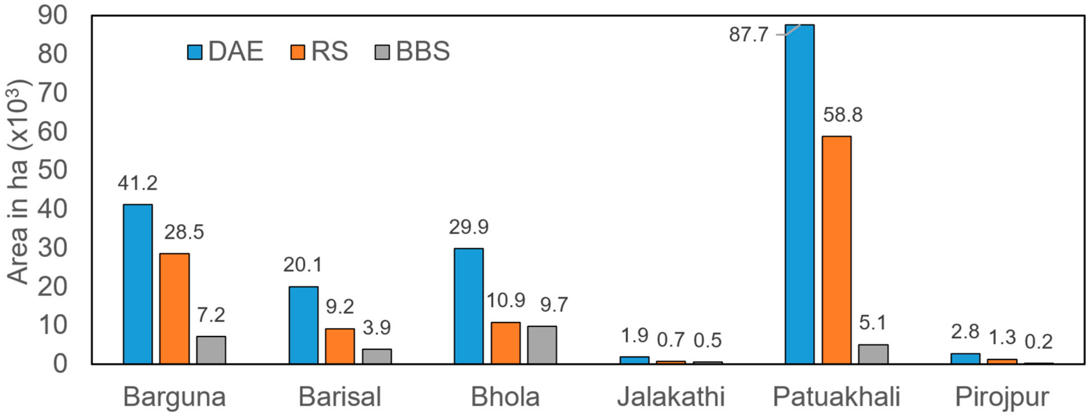
3.4. Comparison with District Level Crop Area Statistics

We compared the data published in the 2018–2019 Agriculture Statistical Yearbook [10] with the data we had obtained from the DAE and the remote sensing based estimates generated in this study at the district level (Figure 12). The BBS data were much lower than then the DAE or the remote sensing based estimates. The remote sensing based estimates followed the trends of the DAE data in all districts, but on average, were about 40% lower than the DAE data.

4. Discussion

Our study area encompassed a portion of coastal South Asia that is dominated by smallholder farming. Average farm size is less than 0.5 ha and average fields size is around 0.1 ha [11,12]. As road infrastructure is poorly developed and most fields can be accessed by foot only, this poses challenges for the collection of in situ data to assess the extent of particular crops and cropland. In order to identify the area of mung bean production in Barisal division, we relied on photos acquired from a manned, low elevation (150–300 m) flying aircraft, ground data collection and visual photo and satellite image interpretation, to create a dataset containing 2358 segments tagged with crop type and another 2034 segments with non-cropland information. To our knowledge, this is the first combination of these methodologies for crop identification in South Asia and Bangladesh [50,51].
Our cropland area estimate of 463,741 ha for the Barisal division is about 79,000 ha lower than the 543,000 ha reported by [15]. As Sentinel data were not available at the time of that study, [15] relied on Landsat 5, 7 and 8 images, with a 30 m GSD, and examined three years of winter rabi season data from 2011 to 2014, while the current study focused on the 2019 winter season. The landscape in this study area was highly fragmented, with tree lined villages, homesteads, rivers and canals. This results in numerous mixed pixels, which in addition to the differences in study years, may have contributed to the difference in the cropland area estimates. Fallow land estimates also differed: we identified 213,832 ha of weedy fallows, whereas [15] study identified only 74,000 ha, located primarily the southern most regions of Barguna and Patuakhali. This difference however was likely due to contrasting definitions of fallowed land. The later study considered only land that was uncropped throughout the entire winter rabi season from December 21 through April 10th as fallow, whereas the current study included land that was fallow from February 6th to April 17th, coinciding with the primary mung bean cultivation period. The large transect of fallow land across Southern Pirojpur, Jhalokati and Barisal district was presumably cropped with grass pea, the fields of which are generally not tilled after harvesting and thereby develop into weedy fallows.
The temporal analysis, represented by four different scenarios, revealed that it would be possible to identify the area planted in early February with a high accuracy (user’s accuracy = 0.96 and producer’s accuracy = 0.93). There was little room for improvement by adding additional images; nevertheless, the highest accuracies were obtained by using images from all four acquisition dates. Estimation of the area planted would be challenging, since the preparation of the in-situ data for training and validation based on an early February satellite image alone would be difficult. Bare soil, i.e., the freshly sown mung bean fields, would be difficult to separate from the weedy fallow fields in false color satellite images. However, estimates and maps of area planted could provide relevant information for food security and disaster monitoring, as high rainfall can cause great damage to mung bean in this region [52].
Our remote sensing based mung bean area estimate of 109,416 ha was about 40% lower than the DAE estimates, but more than four times higher than the 2019 data reported by BBS. Neither of the latter two approaches were able to apply comprehensive systematic sampling, and necessarily make use of expert judgment and estimates in crop reporting. The approach described in the current paper could be a viable alternative, although pixel counting could also be biased unless combined with thorough ground truthing [53], as exemplified in the current study.
While individual crop fields in our study area measured only about 0.08–0.1 ha on average [11,12], the merging of adjacent segments of the same crop types resulted in much larger continuously cropped areas, measuring 1.62 ha on average for mung bean. It is important to note here that the objectives of the current study were to assess total mung bean cropped land; while assessment of the sizes of individual fields cropped to mung bean is an important research priority, it requires further investigation with appropriate methods to develop reliable remotely sensed estimates. Mung bean is grown several months following the recession of the monsoon season and established in February when temperature increases to assure germination. Differences in land elevation, and thus monsoon season flooding depth and duration, greatly affect waterlogging and post-monsoon season soil moisture that limit trafficability of fields, crop species choice and the timing of planting for farmers in coastal Bangladesh [15,54]. The recession of floodwaters after the monsoon and opening of tracts of land that could be cropped in coastal Bangladesh limits the degree of possible crop diversity while also forcing farmers to establish their crops in adjacent fields—which are usually grown with the same crop—that have similar soil moisture levels and trafficability characteristics [15]. Contiguous fields result in patches grown with the same crop type that are much larger than individual fields. This makes it possible to identify crops on fields that on average, measure only 10 pixels with satellite images at a GSD of 10 m. In the case of mung bean, an average patch covered 160 Sentinel-2 pixels. Thus, fragmentation is much lower than what one would expect when considering individual fields. This makes it possible to monitor the area of predominant crops in a smallholder farming setting of coastal South Asia with optical 10 m GSD data.
However, the general applicability of Sentinel-2 data in small holder farming settings in South Asia would have to be further tested, especially in regions where farmers have more options and therefore, crops are more diverse. In the coastal region of Bangladesh, crop choice for the dry winter months is constrained by topography and a lack of proper drainage and irrigation systems, which in turn control where and when the fields can be grown with crops that, unlike rice, do not tolerate flooding. This study demonstrated a method to generate multi-source in situ data and tests the suitability of 10 m GSD Sentinel-2 images for mung bean identification in a smallholder farming setting of South Asia. This effort however did not come without transactions costs—approximately 800 h or 100 work days were required to create the training and test data for mung bean identification. Conversely, future efforts should consider employing alternative methods including crowd-sourcing, perhaps with the aid of a Geo-Wiki platform [46,50,51], or by engaging DAE extension officers in the regular collection of geotagged in situ data of fields cropped to particular species. Such efforts may well be worth the effort to improve estimates of cropped area, and strong multi-institutional collaborations in the assessment and monitoring of cropland in South Asia and could serve as an important example for other regions dominated by a smallholder farming system.

5. Conclusions

By combining imagery obtained by low-elevation (150–300 m) manned aircraft derived photographs, ground truth data and visual interpretation of these data sources together with satellite remotely sensed information, this study generated a representative data set consisting of 2358 tagged mung bean and agricultural land use type segments for the entirety of a 1,364,500 ha region in Barisal division of coastal Bangladesh. Object based classification with the RT algorithm resulted in overall accuracy and Kappa Index of Agreement greater than 0.96. This indicates that Sentinel-2 data with a GSD of 10 m were suitable for the identification of mung bean in the smallholder farming context of South Asia, despite of the predominance of very small field sizes measuring only between 0.08 and 0.10 ha. When merging adjacent segments by crop type, an average patch size for mung bean of 1.6 ha resulted. Thus, in the smallholder farming setting of the coastal zone of Bangladesh, the low crop type fragmentation resulted in patches that on average were about 15 times larger than the individual fields and could be detected with 10 m GSD Sentinel-2 data.

Author Contributions

Conceptualization, M.K., U.S., and T.J.K.; methodology, M.K. and U.S.; software, M.K.; validation, M.K.; formal analysis, M.K.; investigation, M.K., U.S., and T.J.K.; resources, T.J.K.; data curation, M.K.; writing—original draft preparation, M.K. and U.S.; writing—review and editing, M.K., U.S., and T.J.K.; visualization, M.K.; supervision, T.J.K.; project administration, T.J.K.; funding acquisition, T.J.K. All authors have read and agreed to the published version of the manuscript.

Funding

This research was funded by USAID and Bill and Melinda Gates Foundation (BMGF) Cereal System Initiative for South Asia (CSISA).

Acknowledgments

This research was conducted under the USAID and Bill and Melinda Gates Foundation (BMGF) Cereal System Initiative for South Asia (CSISA). This paper does not necessarily represent the views of, and is not endorsed by USAID, BMGF, or the US government, and may not be used for advertising purposes. We thank USAID and MAF Bangladesh for supporting aerial reconnaissance. We also thank the Department of Agriculture Extension (DAE) for recent crop estimation data. Abdul Jalil, Mehedi Hasan and Golam Morshed Rokon assisted in the collection of in situ data. Md. Khaled Hossain, Mutasim Billah and Uttam Barman supported the acquisition of aerial photos and Asif Al Faisal helped with preparing a figure. Mehedi Hasan and Taposh Mollick generated the in situ data set.

Conflicts of Interest

The authors declare no conflict of interest. The funders had no role in the design of the study; in the collection, analyses, or interpretation of data; in the writing of the manuscript, or in the decision to publish the results.

References

  1. GA UN. Transforming Our World: The 2030 Agenda for Sustainable Development; Division for Sustainable Development Goals: New York, NY, USA, 2015. [Google Scholar]
  2. Kubitza, C.; Krishna, V.V.; Schulthess, U.; Jain, M. Estimating adoption and impacts of agricultural management practices in developing countries using satellite data. A scoping review. Agron. Sustain. Dev. 2020, 40, 1–21. [Google Scholar] [CrossRef]
  3. See, L.; Fritz, S.; You, L.; Ramankutty, N.; Herrero, M.; Justice, C.; Becker-Reshef, I.; Thornton, P.; Erb, K.; Gong, P. Improved global cropland data as an essential ingredient for food security. Glob. Food Secur. 2015, 4, 37–45. [Google Scholar] [CrossRef]
  4. Saha, U.R.; Chattapadhayay, A.; Richardus, J.H. Trends, prevalence and determinants of childhood chronic undernutrition in regional divisions of Bangladesh: Evidence from demographic health surveys, 2011 and 2014. PLoS ONE 2019, 14, e0220062. [Google Scholar] [CrossRef] [Green Version]
  5. Miah, M.M.; Alam, Q.; Sarker, A.; Aktar, M. Socio-economic Impact of Pulse Research in Some Selected Areas of Bangladesh. Asia Pac. J. Rural Dev. 2009, 19, 115–142. [Google Scholar] [CrossRef]
  6. Shanmugasundaram, S.; Keatinge, J.; Hughes, J.d.A. The mungbean transformation: Diversifying crops, defeating malnutrition. Proven Successes Agric. Dev. 2009, 381–405. [Google Scholar]
  7. Bilal, A.; Rakha, A.; Butt, M.S.; Shahid, M. Nutritional and physicochemical attributes of cowpea and mungbean based weaning foods. Pak. J. Agric. Sci. 2017, 54, 653–662. [Google Scholar]
  8. Islam, Q.S.; Rahman, M.; Hossain, M.; Hossain, M. Economic analysis of mungbean (vigna radiata) cultivation in some coastal areas of Bangladesh. Bangladesh J. Agric. Res. 2011, 36, 29–40. [Google Scholar] [CrossRef] [Green Version]
  9. Rahman, M.M. Country report: Bangladesh. In Proceedings of the ADBI-APO Workshop on Climate Change and its Impact on Agric, Seoul, Korea, 13–16 December 2011; pp. 1–18. [Google Scholar]
  10. BBS. Statistical Year Book of Bangladesh; Ministry of Planning, Government of the People’s Republic of Bangladesh: Dhaka, Bangladesh, 2019.
  11. Rahman, S.; Rahman, M. Impact of land fragmentation and resource ownership on productivity and efficiency: The case of rice producers in Bangladesh. Land Use Policy 2009, 26, 95–103. [Google Scholar] [CrossRef] [Green Version]
  12. Yang, R.; Ahmed, Z.U.; Schulthess, U.C.; Kamal, M.; Rai, R. Detecting functional field units from satellite images in smallholder farming systems using a deep learning based computer vision approach: A case study from Bangladesh. Remote Sens. Appl. Soc. Environ. 2020, 20, 100413. [Google Scholar] [CrossRef]
  13. Aravindakshan, S.; Krupnik, T.J.; Groot, J.C.; Speelman, E.N.; Amjath-Babu, T.; Tittonell, P. Multi-level socioecological drivers of agrarian change: Longitudinal evidence from mixed rice-livestock-aquaculture farming systems of Bangladesh. Agric. Syst. 2020, 177, 102695. [Google Scholar] [CrossRef]
  14. Haque, S. Salinity problems and crop production in coastal regions of Bangladesh. Pak. J. Bot. 2006, 38, 1359–1365. [Google Scholar]
  15. Krupnik, T.J.; Schulthess, U.; Ahmed, Z.U.; McDonald, A.J. Sustainable crop intensification through surface water irrigation in Bangladesh? A geospatial assessment of landscape-scale production potential. Land Use Policy 2017, 60, 206–222. [Google Scholar] [CrossRef] [Green Version]
  16. Mottaleb, K.A.; Krupnik, T.J.; Erenstein, O. Factors associated with small-scale agricultural machinery adoption in Bangladesh: Census findings. J. Rural Stud. 2016, 46, 155–168. [Google Scholar] [CrossRef] [Green Version]
  17. Defourny, P.; Bontemps, S.; Bellemans, N.; Cara, C.; Dedieu, G.; Guzzonato, E.; Hagolle, O.; Inglada, J.; Nicola, L.; Rabaute, T. Near real-time agriculture monitoring at national scale at parcel resolution: Performance assessment of the Sen2-Agri automated system in various cropping systems around the world. Remote Sens. Environ. 2019, 221, 551–568. [Google Scholar] [CrossRef]
  18. SNAP. ESA Sentinel Application Platform v7.0. Available online: http://step.esa.int (accessed on 15 January 2020).
  19. Gómez, C.; White, J.C.; Wulder, M.A. Optical remotely sensed time series data for land cover classification: A review. ISPRS J. Photogramm. Remote Sens. 2016, 116, 55–72. [Google Scholar] [CrossRef] [Green Version]
  20. Nitze, I.; Schulthess, U.; Asche, H. Comparison of machine learning algorithms random forest, artificial neural network and support vector machine to maximum likelihood for supervised crop type classification. In Proceedings of the 4th Geobia, Rio de Janeiro, Brazil, 7–9 May 2012; pp. 35–40. [Google Scholar]
  21. Breiman, L. Random forests. Mach. Learn. 2001, 45, 5–32. [Google Scholar] [CrossRef] [Green Version]
  22. Rosenblatt, F. The perceptron: A probabilistic model for information storage and organization in the brain. Psychol. Rev. 1958, 65, 386. [Google Scholar] [CrossRef] [Green Version]
  23. Rumelhart, D.E.; Hinton, G.E.; Williams, R.J. Learning representations by back-propagating errors. Nature 1986, 323, 533–536. [Google Scholar] [CrossRef]
  24. Cortes, C.; Vapnik, V. Support-vector networks. Mach. Learn. 1995, 20, 273–297. [Google Scholar] [CrossRef]
  25. Belgiu, M.; Drăguţ, L. Random forest in remote sensing: A review of applications and future directions. ISPRS J. Photogramm. Remote Sens. 2016, 114, 24–31. [Google Scholar] [CrossRef]
  26. Poulton, P.; Dalgliesh, N. Evaluating use of remote sensing for identifying management strategies: Example for small plot farmers during the dry season in southern Bangladesh. In Proceedings of the 14th Agronomy Conference, Adelaide, Australia, 21–25 September 2008; pp. 21–25. Available online: http://www.agronomyaustraliaproceedings.org/images/sampledata/2008/concurrent/agronomy-abroad/5754_poultonpl.pdf (accessed on 4 November 2020).
  27. Schulthess, U.; Krupnik, T.; Ahmed, Z.; McDonald, A. Technology targeting for sustainable intensification of crop production in the delta region of bangladesh. Int. Arch. Photogramm. Remote Sens. Spat. Inf. Sci. 2015. [Google Scholar] [CrossRef] [Green Version]
  28. Schulthess, U.; Timsina, J.; Herrera, J.; McDonald, A. Mapping field-scale yield gaps for maize: An example from Bangladesh. Field Crop Res. 2013, 143, 151–156. [Google Scholar] [CrossRef] [Green Version]
  29. Gumma, M.K.; Thenkabail, P.S.; Maunahan, A.; Islam, S.; Nelson, A. Mapping seasonal rice cropland extent and area in the high cropping intensity environment of Bangladesh using MODIS 500 m data for the year 2010. ISPRS J. Photogramm. Remote Sens. 2014, 91, 98–113. [Google Scholar] [CrossRef]
  30. Shew, A.M.; Ghosh, A. Identifying Dry-Season Rice-Planting Patterns in Bangladesh Using the Landsat Archive. Remote Sens. 2019, 11, 1235. [Google Scholar] [CrossRef] [Green Version]
  31. Singha, M.; Dong, J.; Sarmah, S.; You, N.; Zhou, Y.; Zhang, G.; Doughty, R.; Xiao, X. Identifying floods and flood-affected paddy rice fields in Bangladesh based on Sentinel-1 imagery and Google Earth Engine. ISPRS J. Photogramm. Remote Sens. 2020, 166, 278–293. [Google Scholar] [CrossRef]
  32. Bhagia, N.; Bairagi, G.; Pandagre, S.; Patel, G.; Vyas, S.; Kumar, G.N.; Ramteke, I.; Mesharam, P. National Inventory of Rabi Pulses in India Using Remotely Sensed Data. J. Indian Soc. Remote Sens. 2017, 45, 285–295. [Google Scholar] [CrossRef]
  33. Schulthess, U.; Ahmed, Z.U.; Aravindakshan, S.; Rokon, G.M.; Kurishi, A.A.; Krupnik, T.J. Farming on the fringe: Shallow groundwater dynamics and irrigation scheduling for maize and wheat in Bangladesh’s coastal delta. Field Crop Res. 2019, 239, 135–148. [Google Scholar] [CrossRef]
  34. Islam, M.R. Crop Diversification in Cyclone Sidr Affected Southern Bangladesh; Food and Agriculture Organization of The United Nations: Dhaka, Bangladesh, 2012. [Google Scholar]
  35. Anon. Google Earth Engine Guides. Available online: https://developers.google.com/earth-engine/tutorials/tutorial_api_05 (accessed on 4 November 2020).
  36. Muller-Wilm, U.; Louis, J.; Richter, R.; Gascon, F.; Niezette, M. Sentinel-2 level 2A prototype processor: Architecture, algorithms and first results. In Proceedings of the ESA Living Planet Symposium, Edinburgh, UK, 9–13 September 2013; pp. 9–13. [Google Scholar]
  37. Rouse, J.; Haas, R.; Schell, J.; Deering, D.W. Monitoring vegetation systems in the great plains with ERTS. In Proceedings of the Third ERTS Symposium, Washington, DC, USA, 10–14 December 1973; pp. 309–317. [Google Scholar]
  38. Huete, A.; Didan, K.; Miura, T.; Rodriguez, E.P.; Gao, X.; Ferreira, L.G. Overview of the radiometric and biophysical performance of the MODIS vegetation indices. Remote Sens. Environ. 2002, 83, 195–213. [Google Scholar] [CrossRef]
  39. Gitelson, A.A.; Kaufman, Y.J.; Merzlyak, M.N. Use of a green channel in remote sensing of global vegetation from EOS-MODIS. Remote Sens. Environ. 1996, 58, 289–298. [Google Scholar] [CrossRef]
  40. Huete, A.R. A soil-adjusted vegetation index (SAVI). Remote Sens. Environ. 1988, 25, 295–309. [Google Scholar] [CrossRef]
  41. Escadafal, R. Remote sensing of arid soil surface color with Landsat thematic mapper. Adv. Space Res. 1989, 9, 159–163. [Google Scholar] [CrossRef]
  42. Pouget, M.; Madeira, J.; Le Floch, E.; Kamal, S. Caracteristiques spectrales des surfaces sableuses de la region cotiere nord-ouest de l’Egypte: Application aux donnees satellitaires SPOT. In Journee de Teledetection Caractérisation et Suivi des Milieux Terrestres en Régions Arides et Tropicales; ORSTOM: Paris, France, 1990; Volume 12, pp. 27–39. [Google Scholar]
  43. Gao, B.-C. NDWI—A normalized difference water index for remote sensing of vegetation liquid water from space. Remote Sens. Environ. 1996, 58, 257–266. [Google Scholar] [CrossRef]
  44. McFeeters, S.K. The use of the Normalized Difference Water Index (NDWI) in the delineation of open water features. Int. J. Remote Sens. 1996, 17, 1425–1432. [Google Scholar] [CrossRef]
  45. Baatz, M.; Schäpe, A. Multiresolution Segmentation: An optimization approach for high quality multi-scale image segmentation. In Angewandte Geographische Informationsverarbeitung XII: Beiträge Zum AGIT-Symposium Salzburg; Wichmann Verlag: Karlsruhe, Germany, 2000; pp. 12–23. [Google Scholar]
  46. JeffreyCoker, F.; Basinger, M.; Modi, V. Open Data Kit: Implications for the Use of Smartphone Software Technology for Questionnaire Studies in International Development. Available online: https://qsel.columbia.edu/assets/uploads/blog/2013/06/Open-Data-Kit-Review-Article.pdf (accessed on 4 November 2020).
  47. OpenCV. Random Tree. Available online: https://docs.opencv.org/2.4/modules/ml/doc/random_trees.html?highlight=rtrees (accessed on 4 November 2020).
  48. Congalton, R.G. A review of assessing the accuracy of classifications of remotely sensed data. Remote Sens. Environ. 1991, 37, 35–46. [Google Scholar] [CrossRef]
  49. Cohen, J. A coefficient of agreement for nominal scales. Educ. Psychol. Meas. 1960, 20, 37–46. [Google Scholar] [CrossRef]
  50. Fritz, S.; Fonte, C.C.; See, L. The role of citizen science in earth observation. Remote Sens. 2017, 9, 357. [Google Scholar] [CrossRef] [Green Version]
  51. Fritz, S.; See, L.; Perger, C.; McCallum, I.; Schill, C.; Schepaschenko, D.; Duerauer, M.; Karner, M.; Dresel, C.; Laso-Bayas, J. A global dataset of crowdsourced land cover and land use reference data. Sci. Data 2017, 4, 170075. [Google Scholar] [CrossRef] [Green Version]
  52. Rahman, M.M.; Neogi, M.G.; Mollah, M.F.H.; Salahuddin, A.K.M.; Amin, M.R.; Hamid, A. Socio-Economic and Biophysical Constraints of Dry Season Cropping in Tidal Floodplain of Bangladesh. J. Appl. Agric. Econ. Policy Anal. 2019, 2, 40–46. [Google Scholar]
  53. Waldner, F.; Defourny, P. Where can pixel counting area estimates meet user-defined accuracy requirements? Int. J. Appl. Earth Obs. Geoinf. 2017, 60, 1–10. [Google Scholar] [CrossRef]
  54. Brammer, H. The Physical Geography of Bangladesh; The University Press Limited (UPL): Dhaka, Bangladesh, 2012. [Google Scholar]
Figure 1. Map of Barisal division in costal Bangladesh with its six districts (a). The footprint of the two Sentinel-2 tiles T45QZE and T45QZF, which limit the extent of our study area, is also shown (b).
Remotesensing 12 03688 g001
Figure 2. Workflow of object-based machine learning approach for mung bean classification in Barisal division in coastal Bangladesh.
Remotesensing 12 03688 g002
Figure 3. Availability of Sentinel-2 images acquired during the mung bean growing season from February 6 through April 22 of 2019 over the study area. Images marked with a black bold circle were used for the analyses.
Remotesensing 12 03688 g003
Figure 4. (a) The flight path of the S2-AEC sea plane used for crop field surveillance at 150–300 m height on 25 March 2019. A mung bean field is shown in (b). Panels (c), mostly mung bean, and (d), with lush green rice fields, are photos taken from the aircraft. Locations are indicated on (a).
Remotesensing 12 03688 g004
Figure 5. Training sample preparation workflow: We started with an aerial image (a), which we then related to the Google Earth background imagery (b). Subsequently, a field technician identified the crops shown on the aerial image in the field with the Open Data Kit (ODK); (c). In a last step, we linked the ODK data points with crop type information to segments based on Sentinel-2 images (d).
Remotesensing 12 03688 g005
Figure 6. Time course of mean normalized difference vegetation (NDVI) development of the four major crop types during the mung bean growing season from February 6 through April 27 of 2019 in Barisal division of coastal Bangladesh. Data were derived from the segments of the in situ data set created for the crop classification. Bars represent one standard deviation.
Remotesensing 12 03688 g006
Figure 7. Segments overlaid on a sequence of four false color Sentinel-2 images acquired during the mung bean growing season from February 6 through 17 April 2019. Average size of a segment is 0.02 ha. On the February and March images, bare soil or soil with little vegetation is shown in light turquoise colors. These areas were sown with mung bean in early February and appear in dark pink color in the March 28 and mid-April images.
Remotesensing 12 03688 g007
Figure 8. Relative importance scores of the top 20 index by image acquisition date combinations used for the identification of the crops by mid-April with a random tree algorithm. Imagery acquired on 4 dates between February 6 and mid-April, 2019 was used to calculate 9 indices, resulting in 36 data layers. Layers labeled with an acquisition date of April 17 are based on the median of cloud-free pixels acquired on April 7, 17 and 22.
Remotesensing 12 03688 g008
Figure 9. Change of user’s and producer’s accuracies over time for four crop types grown in the Barisal division of Bangladesh in 2019. The accuracies are based on different sequences of images, starting with one image acquired on February 6 and ending with 4 image acquisition dates by mid-April.
Remotesensing 12 03688 g009
Figure 10. Histograms and box and whisker plots of the areas of contiguous patches grown with the same crop type identified during the mung bean growing season from February 6 through April 17, 2019 in Barisal division of Coastal Bangladesh. The patches were created by merging segments with common borders labeled with the same crop type.
Remotesensing 12 03688 g010
Figure 11. (a) Classified spatial distribution of the four major crop types cultivated in the Barisal division of coastal Bangladesh during the mung bean growing season from February 6 through 17 April 2019. The locations of panels (b,c) are marked with a black rectangle on (a).
Remotesensing 12 03688 g011
Figure 12. Area estimates for mung bean production by district in Barisal division in coastal Bangladesh during the mung bean growing season from February 6 through 17 April 2019. Data were either obtained from Bangladesh Bureau of Statistics (BBS) and the Department of Agricultural Extension (DAE) or generated with remote sensing (RS) as described in the methodology section.
Remotesensing 12 03688 g012
Table 1. Vegetation, soil and water indices derived from Sentinel-2 images. The resulting information layers were used for segmentation and classification images during the mung bean growing season from February 6 through April 17 of 2019 in Barisal division of coastal Bangladesh.
IndicesNameFormula/FunctionTypeSource
NDVINormalized Difference Vegetation Index(B8 − B4)/(B8 + B4)Vegetation[37]
EVIEnhanced Vegetation index2.5 × (B8 − B4)/(1 + B8 + 6 × B4 − 7.5 × B2 + 10,000)Vegetation[38]
GNDVIGreen Normalized Difference Vegetation Index(B8 − B3)/(B8 + B3)Vegetation[39]
SAVISoil Adjusted Vegetation Index(1 + L) × (B8 − B4)/(B8 + B4 + L)Vegetation[40]
BIBrightness Indexsqrt(((B4 × B4) + (B3 × B3))/2)Soil[41]
BI2The second Brightness Indexsqrt(((B4 × B4) + (B3 × B3) + (B8 × B8))/3)Soil[41]
CIColor Index(B4 − B3)/(B4 + B3)Soil[42]
NDWINormalized Difference Water Index(B8 − B12)/(B8 + B12)Water[43]
NDWI2The second Normalized Difference Water Index(B3 − B8)/(B3 + B8)Water[44]
Table 2. Number of training and test samples for each class investigated. In-situ data that were collected in the field with the Open Data Kit (ODK) contain the term ODK in their label.
ClassODK + AerialODK + Satellite ImageAerial + Satellite ImageSatellite Image + Google Earth + ExperienceTotal SamplesTrainingTest (without ODK Data)
Non-crop00204183020341356678
Fallow349678179900600300
Mung bean135417240900600300
Other crop003141724824
Rice1116234180441294147
Total1806618712230439228981449
Table 3. Results of the segment based cropland vs. non-cropland classification for Barisal division in the spring of 2019.
ClassNon-CropCropTotalUser’s Accuracy
Non-crop66276690.99
Crop167797950.98
Total6787861464
Producer’s accuracy0.980.99
Kappa Index of Agreement: 0.97; Overall Accuracy: 0.98.
Table 4. Results of the segment based identification of the major crop types grown in the Barisal division in the period between February and April 2019.
ClassOther CropMung BeanRiceFallowTotalUser’s Accuracy
Other crop20002220.91
Mung bean0297063030.98
Rice0014301431.00
Fallow2302892940.98
Total22300143297762
Producer’s accuracy0.910.991.000.97
Kappa Index of Agreement: 0.96; Overall Accuracy: 0.97.
Publisher’s Note: MDPI stays neutral with regard to jurisdictional claims in published maps and institutional affiliations.

