Figure 1.
LiDAR data coverage published in the year 2020.
Figure 1.
LiDAR data coverage published in the year 2020.
Figure 2.
Workflow of the methodology followed to evaluate the influence of the density.
Figure 2.
Workflow of the methodology followed to evaluate the influence of the density.
Figure 3.
Point cloud filtering process: (a) original, (b) after removing points belonging to the ground, (c) after removing points belonging to vegetation areas, (d) after removing points belonging to building façades, (e) after removing noise points.
Figure 3.
Point cloud filtering process: (a) original, (b) after removing points belonging to the ground, (c) after removing points belonging to vegetation areas, (d) after removing points belonging to building façades, (e) after removing noise points.
Figure 4.
Estimation of the projected area of a roof: (a) through the digitalization of the aerial orthophotography; (b) through the automatic computation of the boundary of the point cloud.
Figure 4.
Estimation of the projected area of a roof: (a) through the digitalization of the aerial orthophotography; (b) through the automatic computation of the boundary of the point cloud.
Figure 5.
Projected area of reference: area distribution of the different cases of study.
Figure 5.
Projected area of reference: area distribution of the different cases of study.
Figure 6.
Example of residential building roofs used for the evaluation of the effect of the point cloud density in the surface computation error: (a) <200 m2, (b) >200 m2.
Figure 6.
Example of residential building roofs used for the evaluation of the effect of the point cloud density in the surface computation error: (a) <200 m2, (b) >200 m2.
Figure 7.
Example of industrial building roofs used for the evaluation of the effect of the point cloud density in the surface computation error: (a) <200 m2, (b) >200 m2.
Figure 7.
Example of industrial building roofs used for the evaluation of the effect of the point cloud density in the surface computation error: (a) <200 m2, (b) >200 m2.
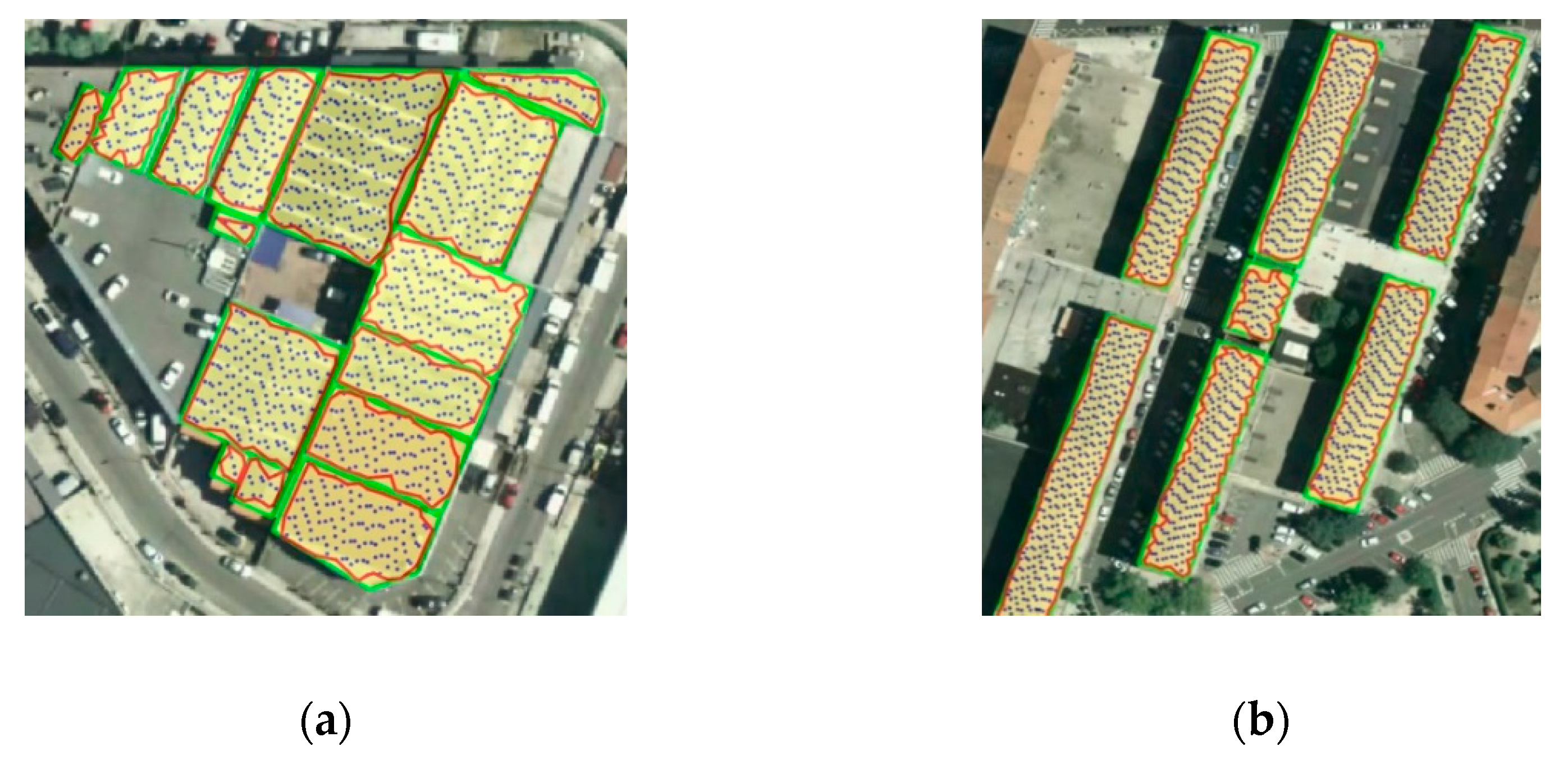
Figure 8.
Graphic results of the projected area of reference defined from aerial orthophotographs (green line) and projected area computed from point cloud (red line): (a) industrial and (b) residential.
Figure 8.
Graphic results of the projected area of reference defined from aerial orthophotographs (green line) and projected area computed from point cloud (red line): (a) industrial and (b) residential.
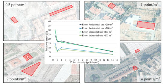
Figure 9.
Mean relative error (%) for buildings with a surface < 200 m2 and > 200 m2: (a) industrial use (b) residential use.
Figure 9.
Mean relative error (%) for buildings with a surface < 200 m2 and > 200 m2: (a) industrial use (b) residential use.
Figure 10.
Recall (%) for the different the point cloud densities depending on the use of the building and the area of the roof.
Figure 10.
Recall (%) for the different the point cloud densities depending on the use of the building and the area of the roof.
Figure 11.
F-score (%) for the different the point cloud densities depending on the use of the building and the area of the roof.
Figure 11.
F-score (%) for the different the point cloud densities depending on the use of the building and the area of the roof.
Figure 12.
Solar climate zones according to the Spanish Technical Construction Code.
Figure 12.
Solar climate zones according to the Spanish Technical Construction Code.
Figure 13.
Mean relative error (%) in the rooftop area calculated for the different the point cloud densities depending on the use of the building and the area of the roof.
Figure 13.
Mean relative error (%) in the rooftop area calculated for the different the point cloud densities depending on the use of the building and the area of the roof.
Figure 14.
Average daily PV energy production per square meter loss (Wh/m2) for industrial buildings with an area smaller than 200 m2: (a) flat roof, (b) gable roof.
Figure 14.
Average daily PV energy production per square meter loss (Wh/m2) for industrial buildings with an area smaller than 200 m2: (a) flat roof, (b) gable roof.
Figure 15.
Average daily PV energy production per square meter loss (Wh/m2) for industrial buildings with an area bigger than 200 m2: (a) flat roof, (b) gable roof.
Figure 15.
Average daily PV energy production per square meter loss (Wh/m2) for industrial buildings with an area bigger than 200 m2: (a) flat roof, (b) gable roof.
Figure 16.
Average daily PV energy production per square meter loss (Wh/m2) for residential buildings with an area smaller than 200 m2: (a) gable roof, (b) hipped roof.
Figure 16.
Average daily PV energy production per square meter loss (Wh/m2) for residential buildings with an area smaller than 200 m2: (a) gable roof, (b) hipped roof.
Figure 17.
Average daily PV energy production per square meter loss (Wh/m2) for residential buildings with a surface bigger than 200 m2: (a) gable roof, (b) hipped roof.
Figure 17.
Average daily PV energy production per square meter loss (Wh/m2) for residential buildings with a surface bigger than 200 m2: (a) gable roof, (b) hipped roof.
Table 1.
Main characteristics of data derived from the National Plan for Aerial Orthophotography (PNOA) Project. Data offered by the Spanish National Geographic Institute on their web page.
Table 1.
Main characteristics of data derived from the National Plan for Aerial Orthophotography (PNOA) Project. Data offered by the Spanish National Geographic Institute on their web page.
| Product | Flight GSD 1 (cm) | GSD Orthophoto (cm) | Planimetric Accuracy in Orthophoto (m) |
|---|
| PNOA 50 cm | 45 | 50 | RMSExy 2 ≤ 1.00 |
| PNOA 25 cm | 22 | 25 | RMSExy ≤ 0.50 |
Table 2.
Technical characteristics of the point clouds resulting from PNOA-LiDAR first and second coverages. Data offered by the Spanish National Geographic Institute through their web page.
Table 2.
Technical characteristics of the point clouds resulting from PNOA-LiDAR first and second coverages. Data offered by the Spanish National Geographic Institute through their web page.
| Coverage | Density (Points/m2) | Elevation Accuracy (m) | Elevation Precision (m) | Estimated Planimetric Accuracy (m) |
|---|
| First | 0.5 | RMSEz ≤ 0.4 | RMSEz ≤ 0.2–0.4 | ≤ 0.3 |
| Second | 1, 2 and 14 | RMSEz ≤ 0.2 | RMSEz ≤ 0.15–0.2 | ≤ 0.3 |
Table 3.
Buildings selected for the different cases.
Table 3.
Buildings selected for the different cases.
| Case | Industrial Building | Residential Building |
|---|
| Case 1 | 35 | 25 |
| Case 2 | 42 | 34 |
| Case 3 | 43 | 36 |
Table 4.
Main features of the first coverage LiDAR data.
Table 4.
Main features of the first coverage LiDAR data.
| Case | Flight Date | Laser Scanner | Density (Points/m2) | RMSE xy (m) | RMSE z (m) |
|---|
| Case 1 | 2010 | Leica ALS50 | 0.5 | 0.30 | 0.40 |
| Case 2 | 2010 | Leica ALS50 | 0.5 | 0.30 | 0.40 |
| Case 3 | 2012 | Leica ALS60 | 0.5 | 0.30 | 0.20 |
Table 5.
Main features of the second coverage LiDAR data.
Table 5.
Main features of the second coverage LiDAR data.
| Case | Flight Date | Laser Scanner | Density (Points/m2) | RMSE xy (m) | RMSE z (m) |
|---|
| Case 1 | 2017 | Leica ALS80 | 1 | 0.20 | 0.15 |
| Case 2 | 2016 | Leica ALS80 | 2 | 0.30 | 0.20 |
| Case 3 | 2017 | Leica SPL100 | 14 | 0.20 | 0.15 |
Table 6.
Average RMSE (m2) per point cloud density for industrial buildings.
Table 6.
Average RMSE (m2) per point cloud density for industrial buildings.
| | 0.5 Point/m2 | 1 Point/m2 | 2 Points/m2 | 14 Points/m2 |
|---|
| Surface < 200 m2 | 26 | 15 | 20 | 5 |
| Surface > 200 m2 | 68 | 36 | 47 | 13 |
Table 7.
Average RMSE (m2) per point cloud density for residential buildings.
Table 7.
Average RMSE (m2) per point cloud density for residential buildings.
| | 0.5 Point/m2 | 1 Point/m2 | 2 Points/m2 | 14 Points/m2 |
|---|
| Surface < 200 m2 | 30 | 19 | 21 | 7 |
| Surface > 200 m2 | 88 | 38 | 62 | 20 |
Table 8.
Mean computation time (s) per point cloud density for industrial buildings.
Table 8.
Mean computation time (s) per point cloud density for industrial buildings.
| | 0.5 Point/m2 | 1 Point/m2 | 2 Points/m2 | 14 Points/m2 |
|---|
| Number of points | 1126 | 2463 | 6876 | 48,399 |
| Mean computation time | 4 | 8 | 13 | 90 |
Table 9.
Mean computation time (s) per point cloud density for residential buildings.
Table 9.
Mean computation time (s) per point cloud density for residential buildings.
| | 0.5 Point/m2 | 1 Point/m2 | 2 Points/m2 | 14 Points/m2 |
|---|
| Number of points | 1048 | 2660 | 3641 | 46,863 |
| Mean computation time | 3 | 7 | 6 | 74 |
Table 10.
Annual average daily global solar radiation (H).
Table 10.
Annual average daily global solar radiation (H).
| Solar Climate Zones | Solar Radiation (kWh/m2) |
|---|
| I | H < 3.8 |
| II | 3.8 ≤ H < 4.2 |
| III | 4.2 ≤ H < 4.6 |
| IV | 4.6 ≤ H < 5.0 |
| V | H ≥ 5.0 |
Table 11.
Average altitude of the different study cases in the calculation of solar energy.
Table 11.
Average altitude of the different study cases in the calculation of solar energy.
| Solar Climate Zones | City | Average Altitude (m) |
|---|
| I | A Coruña | 22 |
| II | Pamplona | 450 |
| III | Zamora | 652 |
| IV | Ciudad Real | 628 |
| V | Almería | 27 |
Table 12.
Average daily electrical energy loss (kWh) due to the error in the estimation of the rooftop area for different point cloud densities: industrial buildings with a flat roof of 100 m2.
Table 12.
Average daily electrical energy loss (kWh) due to the error in the estimation of the rooftop area for different point cloud densities: industrial buildings with a flat roof of 100 m2.
| Solar Climate Zones | RMSE (kWh) |
|---|
| 0.5 Point/m2 | 1 Point/m2 | 2 Points/m2 | 14 Points/m2 |
|---|
| Zone 1 | 19 | 11 | 10 | 4 |
| Zone 2 | 20 | 12 | 11 | 4 |
| Zone 3 | 22 | 13 | 12 | 4 |
| Zone 4 | 23 | 14 | 12 | 5 |
| Zone 5 | 26 | 15 | 14 | 5 |
Table 13.
Average daily electrical energy loss (kWh) due to the error in the estimation of the rooftop area for different point cloud densities: industrial buildings with a flat roof of 400 m2.
Table 13.
Average daily electrical energy loss (kWh) due to the error in the estimation of the rooftop area for different point cloud densities: industrial buildings with a flat roof of 400 m2.
| Solar Climate Zones | RMSE (kWh) |
|---|
| 0.5 Point/m2 | 1 Point/m2 | 2 Points/m2 | 14 Points/m2 |
|---|
| Zone 1 | 29 | 15 | 22 | 6 |
| Zone 2 | 31 | 16 | 23 | 7 |
| Zone 3 | 34 | 18 | 25 | 7 |
| Zone 4 | 35 | 18 | 26 | 8 |
| Zone 5 | 40 | 21 | 29 | 9 |
Table 14.
Average daily electrical energy loss (kWh) due to the error in the estimation of the rooftop area for different point cloud densities: industrial buildings with a gable roof of 100 m2.
Table 14.
Average daily electrical energy loss (kWh) due to the error in the estimation of the rooftop area for different point cloud densities: industrial buildings with a gable roof of 100 m2.
| Solar Climate Zones | RMSE (kWh) |
|---|
| 0.5 Point/m2 | 1 Point/m2 | 2 Points/m2 | 14 Points/m2 |
|---|
| Zone 1 | 9 | 5 | 5 | 1 |
| Zone 2 | 9 | 5 | 5 | 1 |
| Zone 3 | 10 | 6 | 6 | 1 |
| Zone 4 | 11 | 6 | 6 | 2 |
| Zone 5 | 12 | 7 | 7 | 2 |
Table 15.
Average daily electrical energy loss (kWh) due to the error in the estimation of the rooftop area for different point cloud densities: industrial buildings with a gable roof of 400 m2.
Table 15.
Average daily electrical energy loss (kWh) due to the error in the estimation of the rooftop area for different point cloud densities: industrial buildings with a gable roof of 400 m2.
| Solar Climate Zones | RMSE (kWh) |
|---|
| 0.5 Point/m2 | 1 Point/m2 | 2 Points/m2 | 14 Points/m2 |
|---|
| Zone 1 | 14 | 8 | 10 | 3 |
| Zone 2 | 15 | 8 | 11 | 3 |
| Zone 3 | 16 | 9 | 12 | 3 |
| Zone 4 | 17 | 9 | 12 | 3 |
| Zone 5 | 19 | 10 | 14 | 3 |
Table 16.
Average daily PV energy production loss (kWh) due to the error in the estimation of the rooftop area for different point cloud densities: residential building with a gable roof of 100 m2.
Table 16.
Average daily PV energy production loss (kWh) due to the error in the estimation of the rooftop area for different point cloud densities: residential building with a gable roof of 100 m2.
| Solar Climate Zones | RMSE (kWh) |
|---|
| 0.5 Point/m2 | 1 Point/m2 | 2 Points/m2 | 14 Points/m2 |
|---|
| Zone 1 | 8 | 5 | 5 | 1 |
| Zone 2 | 8 | 5 | 5 | 1 |
| Zone 3 | 9 | 6 | 6 | 1 |
| Zone 4 | 9 | 6 | 6 | 2 |
| Zone 5 | 10 | 7 | 7 | 2 |
Table 17.
Average daily PV energy production loss (kWh) due to the error in the estimation of the rooftop area for different point cloud densities: residential building with a gable roof of 400 m2.
Table 17.
Average daily PV energy production loss (kWh) due to the error in the estimation of the rooftop area for different point cloud densities: residential building with a gable roof of 400 m2.
| Solar Climate Zones | RMSE (kWh) |
|---|
| 0.5 Point/m2 | 1 Point/m2 | 2 Points/m2 | 14 Points/m2 |
|---|
| Zone 1 | 19 | 9 | 13 | 4 |
| Zone 2 | 20 | 9 | 13 | 4 |
| Zone 3 | 22 | 10 | 15 | 4 |
| Zone 4 | 23 | 11 | 15 | 5 |
| Zone 5 | 26 | 12 | 17 | 5 |
Table 18.
Average daily PV energy production loss (kWh) due to the error in the estimation of the rooftop area for different point cloud densities: residential building with a hipped roof of 100 m2.
Table 18.
Average daily PV energy production loss (kWh) due to the error in the estimation of the rooftop area for different point cloud densities: residential building with a hipped roof of 100 m2.
| Solar Climate Zones | RMSE (kWh) |
|---|
| 0.5 Point/m2 | 1 Point/m2 | 2 Points/m2 | 14 Points/m2 |
|---|
| Zone 1 | 5 | 4 | 4 | 1 |
| Zone 2 | 5 | 4 | 4 | 1 |
| Zone 3 | 6 | 4 | 4 | 1 |
| Zone 4 | 6 | 5 | 5 | 2 |
| Zone 5 | 7 | 5 | 5 | 2 |
Table 19.
Average daily PV energy production loss (kWh) due to the error in the estimation of the rooftop area for different point cloud densities: residential building with a hipped roof of 400 m2.
Table 19.
Average daily PV energy production loss (kWh) due to the error in the estimation of the rooftop area for different point cloud densities: residential building with a hipped roof of 400 m2.
| Solar Climate Zones | RMSE (kWh) |
|---|
| 0.5 Point/m2 | 1 Point/m2 | 2 Points/m2 | 14 Points/m2 |
|---|
| Zona 1 | 13 | 6 | 9 | 3 |
| Zona 2 | 13 | 7 | 9 | 3 |
| Zona 3 | 15 | 7 | 10 | 3 |
| Zona 4 | 15 | 8 | 11 | 3 |
| Zona 5 | 17 | 9 | 12 | 3 |
Table 20.
The results of quality analysis of building outline extraction for different point cloud densities (1 cm, 2.5 cm, 5 cm, 10 cm, 20 cm) for a direct approach.
Table 20.
The results of quality analysis of building outline extraction for different point cloud densities (1 cm, 2.5 cm, 5 cm, 10 cm, 20 cm) for a direct approach.
| | Point Density (Points/m2) |
|---|
| | 10,000 Points/m2 | 1600 Points/m2 | 400 Points/m2 | 100 Points/m2 | 25 Points/m2 |
|---|
| Precision (%) | 97.94 | 97.95 | 97.94 | 97.72 | 97.31 |
| Recall (%) | 99.30 | 99.25 | 99.29 | 99.52 | 99.47 |
| F-score (%) | 97.26 | 97.23 | 97.29 | 97.26 | 96.80 |


 ,
, 


