Article

Investigating the Uncertainties Propagation Analysis of CO2 Emissions Gridded Maps at the Urban Scale: A Case Study of Jinjiang City, China

1
Key Laboratory of Urban Environment and Health, Institute of Urban Environment, Chinese Academy of Sciences, Xiamen 361021, China
2
University of Chinese Academy of Sciences, Beijing 100049, China
3
Faculty of Geo-Information Science and Earth Observation (ITC), University of Twente, 7500AE Enschede, The Netherlands
4
Ningbo Urban Environment Observation and Research Station-NUEORS, Chinese Academy of Sciences, Ningbo 315800, China
5
Key Laboratory of Urban Pollutant Conversion, Institute of Urban Environment, Chinese Academy of Sciences, Xiamen 361021, China
6
Stuart Weitzman School of Design, University of Pennsylvania, Philadelphia, PA 19104, USA
*
Author to whom correspondence should be addressed.
These authors contributed equally to this work.
Remote Sens. 2020, 12(23), 3932; https://doi.org/10.3390/rs12233932
Submission received: 17 November 2020 / Revised: 26 November 2020 / Accepted: 27 November 2020 / Published: 30 November 2020
(This article belongs to the Special Issue Integrating Remote Sensing and Urban Informatics)

Abstract

:
Gridded CO2 emission maps at the urban scale can aid the design of low-carbon development strategies. However, the large uncertainties associated with such maps increase policy-related risks. Therefore, an investigation of the uncertainties in gridded maps at the urban scale is essential. This study proposed an analytic workflow to assess uncertainty propagation during the gridding process. Gridded CO2 emission maps were produced using two resolutions of geospatial datasets (e.g., remote sensing satellite-derived products) for Jinjiang City, China, and a workflow was applied to analyze uncertainties. The workflow involved four submodules that can be used to evaluate the uncertainties of CO2 emissions in gridded maps, caused by the gridded model and input. Fine-resolution (30 m) maps have a larger spatial variation in CO2 emissions, which gives the fine-resolution maps a higher degree of uncertainty propagation. Furthermore, the uncertainties of gridded CO2 emission maps, caused by inserting a random error into spatial proxies, were found to decrease after the gridding process. This can be explained by the “compensation of error” phenomenon, which may be attributed to the cancellation of the overestimated and underestimated values among the different sectors at the same grid. This indicates a nonlinear change between the sum of the uncertainties for different sectors and the actual uncertainties in the gridded maps. In conclusion, the present workflow determined uncertainties were caused by the gridded model and input. These results may aid decision-makers in establishing emission reduction targets, and in developing both low-carbon cities and community policies.

Graphical Abstract

1. Introduction

Cities play an essential role in low-carbon development [1] since they accommodate half of the global population, and account for three quarters of both global energy consumption and greenhouse gas emissions [2]. Understanding the spatiotemporal distributions of CO2 emissions from anthropogenic activities is essential for their mitigation [3,4]. Geospatial datasets obtained from multiple sources (e.g., remote sensing satellites, crowd-sourcing data, location-based service data, and sensors data) are increasing in number, which enables the accurate measurement of the spatiotemporal dynamics of CO2 emissions. However, large uncertainties in estimating CO2 emissions at the urban scale, reduce the efficacy of mitigation policies [5]. For instance, uncertainties (50–100%) at the state and urban scales in the USA [6] are greater than the emission reduction target for New York City [7]. High uncertainty (42.96%) has also been reported between consumption-based (142 Mt) and production-based emissions (81 Mt) in Beijing, China [8]; with a value nearly equal to the emission reduction target [9]. Uncertainties for medium and small cities in China are generally greater than 40 and 20%, respectively [8].
Estimating CO2 emissions at the urban scale, including both un-gridded (i.e., administrative unit maps[10,11,12,13,14]) and gridded maps, cannot avoid the propagation of uncertainties from input to result, which highlights the importance of being aware of uncertainty estimation, especially in gridded maps due to its implications for the precision mitigation of CO2 emissions. Two primary sources of uncertainties for the CO2 emission gridding process can be identified as the uncertainties caused by the gridded model (geoprocessing analysis), and those caused by the input. Previous studies have focused on the uncertainties caused by the input. For example, Gately et al. (2017) investigated the two detailed main sources of uncertainties for input: (1) the total emissions estimations, and (2) the spatial (or temporal) distributions of proxies (i.e., proxies refer to the potential geospatial datasets that could reflect and be used to generate the spatial or temporal distribution of CO2 emissions) [5]. Uncertainties in total emission estimations have been analyzed and reported in several studies on un-gridded maps [12,15]. These uncertainties have been attributed to activity levels (energy consumption or industrial production, e.g., statistical data of energy consumption) and emission factors [16]. A previous study reported a 20% difference between the aggregated statistical data on energy in 30 provinces, and the national statistical data on energy for China [16]. Moreover, the default global emission factors do not account for the actual emission scenarios among different countries, and tend to overestimate the total emissions when compared to local reports (e.g., a 14% emission bias reported in China) [17]. Furthermore, uncertainties in the total emission estimations vary at different scales. Previous studies have reported low uncertainty (−6 to 6%) in the total emissions estimations for 24 Chinese cities in 2010, medium uncertainty (−9 to 11%) in the national CO2 emissions estimate for China in 2005, and high uncertainty (−18.75 to 18.75%) in the global CO2 emissions estimate from combustion sources in 2007 [15,18,19]. For the uncertainties in the spatial (or temporal) distributions of proxies, these uncertainties mostly occur in gridded maps, and can be attributed to the aggregated effects of their spatial resolutions, and the inaccurate spatial patterns of emissions [5]. The aggregated effects misestimate emissions at the grid-cell level, because emissions are generally generated at a spatial scale coarser than that of the actual source activities. For example, a comparison of the Fossil Fuel Data Assimilation System, the Open-Source Data Inventory for Anthropogenic CO2, the Emissions Database for Global Atmospheric Research (EDGAR), and the Anthropogenic Carbon Emissions System indicated significant differences in CO2 emissions at regional (20%) and city scales (50–250%) [5]. Additionally, the inaccurate spatial patterns of emissions of spatial proxies mean that the uncertainty exists in a digital representation (e.g., uncertainties in retrieval products, uncertainties in geoprocessing process, or the low-quality satellite imagery due to cloud mask), or that spatial proxies cannot entirely reflect the spatial distribution of CO2 emissions (e.g., population density gridded maps) [20]. For instance, the gridded uncertainties in the CDIAC data were based on uncertainties in the spatial proxies, which were attributed to the transformation of the coordinate system (29–112 km per degree at different latitudes, 0–73.87%) and the raster representation (0–100%). The results indicated that uncertainties in the CDIAC map ranged from 4 to 190% [21].
However, to our knowledge, few studies have investigated the uncertainties caused by the gridded model. Most of the existing detailed gridded CO2 emission maps have been classified into two categories, namely the “global downscaled” and “bottom-up” approaches [22]. The global downscaled approach uses spatial proxies, such as population data and nighttime light imagery, to determine the total global, national, and regional emissions over a defined space and time domain [23]. Whereas, the bottom-up approach focuses on spatiotemporally explicit gridded CO2 emission maps based on direct flux monitoring (eddy covariance measurements) and sector emission data from various sources, such as transportation, industry, and commercial buildings [22]. In both the allocated model of the global downscaled approach, and the transformed model of the bottom-up approach, may exist model structural error, leading to uncertainties. Furthermore, uncertainties existing in non-spatial and spatial data will subsequently propagate through the gridding process of CO2 emissions. Generally, the uncertainties propagated through the gridding process are ultimately enlarged/reduced. This may cause misleading findings for CO2 emissions-related studies.
Thus, the quantification of uncertainties at the urban scale is central to research on CO2 emissions [5]. Previous methodologies for the quantification of uncertainties of CO2 emissions could be categorized into two main types: using Monte Carlo simulations, or using the inventory comparison method. Monte Carlo simulations can be used to estimate uncertainties in total emission estimations by generating samples according to the probability distribution function, and prior coefficients of variance for activity levels and emission factors [15,18,19]. Previous studies reported prior coefficients of variance for activity levels, ranging from 5 to 30% for different sectors [15,19]. The coefficients of variance for emission factors were primarily based on Intergovernmental Panel on Climate Change guidelines [24]. The existing Monte Carlo simulations can estimate the total uncertainties but lack the spatial distribution of uncertainties to enable identifying both the high-emission and low-uncertainty areas. The inventory comparison method is a commonly used method for evaluating the uncertainties in spatial (or temporal) distribution of proxies by comparing the gridded maps with other open products. The inventory comparison method [5] can be used to evaluate uncertainties in the sum of all cell values, and to subsequently draw uncertainty distribution maps. There is a study that compared the National Bureau of Statistics of China, EDGAR, and Fossil Fuel Data Assimilation System with the China High Resolution Emission Database (CHRED) at two levels, and demonstrated strong correlations (correlation coefficients of 0.58–0.86) between CHRED and the other products [25]. The total emissions estimate obtained from high-resolution mapping methods (7.83 Pg·C·yr−1) was similar to that obtained by the International Energy Agency (7.873 Pg·C·yr−1) [18]. The inventory comparison method has limited applications because of the lack of emission inventories at the urban scale. Furthermore, different accounting scopes among the open gridded CO2 emission inventories can also cause incorrect uncertainty evaluation results.
To address the above mentioned issue, an analytic workflow was proposed to analyze the propagated uncertainties caused by the gridded model and the input for gridded CO2 emission maps. The present workflow used four sub-modules based on Monte Carlo simulations and a bootstrap sampling method to analyze uncertainties, without other detailed open emission inventories. Two of the submodules obtained the corresponding uncertainty of each grid value, generated the uncertainty map caused by the gridded model, and the uncertainties for the sum of each cell (also referred to as propagated uncertainties caused by the model); the other submodules generated the uncertainty distribution maps based on the total emission estimations and spatial proxies (also referred to as propagated uncertainties caused by input). We regarded the gridded maps of CO2 emissions constructed in previous studies as a case study, and applied the workflow to estimate the uncertainties [26,27,28,29]. The estimation of different uncertainties helps decision makers in formulating relevant policies. Uncertainties in total emission estimations aid the determination of emission reduction targets, the corresponding risks for cities and enterprises, and significant emission sources. Uncertainty maps could help to identify locations suitable for developing low-carbon communities. Therefore, this workflow can be adopted in other studies which focus on urban-scale CO2 emissions. Additionally, the estimation of different sources of uncertainty could improve emission-reduction policies.

2. Materials and Methods
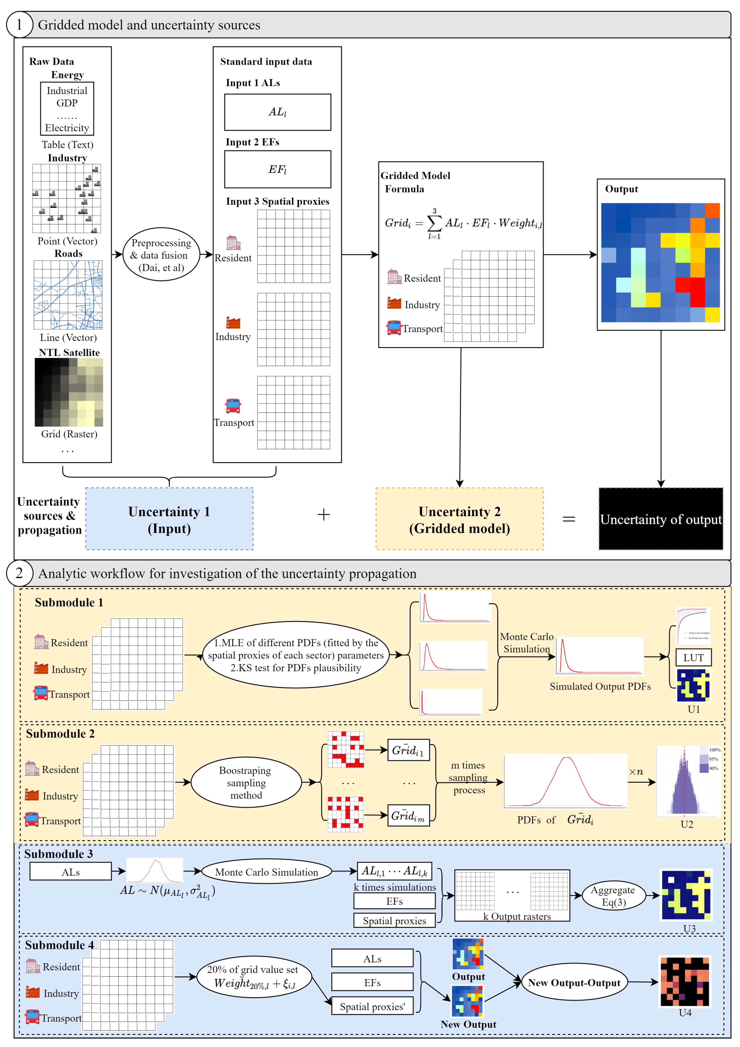
2.1. Overview

Taking Jinjiang in 2013 as the case study, gridded maps of annual CO2 emissions were produced with sizes of 30 m and 500 m using two multi-sources geospatial datasets of corresponding resolution, including satellite (e.g., night light imagery), vector data (e.g., road network, town-level populations), and satellite-derived products (e.g., digital elevation model). Our goal was to quantify the uncertainties caused by the gridded model, and inputs of the gridded CO2 emission maps at the urban scale. We proposed an analytic workflow based on the Monte Carlo simulation and bootstrap sampling method. The workflow included four different submodules, described in Section 2.3.

2.2. The Description of the Case Data

The CO2 emission gridded maps of Jinjiang (E 118°24′–118°43′, N 24°30′–24°54′), a southeastern city in China (Area 649 km2), were constructed based on geospatial datasets (e.g., remote sensing satellite-derived products) from previous studies [26,28]. Jinjiang is one of the most developed counties in China; yet, it represents the local urbanization mode, with fast economic growth and urban sprawl, a stable permanent population, and a large floating population. The gridded maps were constructed using a general hybrid approach, based on global downscaled and bottom-up elements (e.g., industrial areas). In the previous studies, the first step calculated the total (sum of emissions from three sectors below), residential, industrial (except the energy consumption of the electrical production department), and transport emissions using energy consumption values within the urban geographic boundary of Jinjiang City in 2013, and the corresponding emission factors. The next step was generating three corresponding spatial proxies of each sector: resident (refers to population density gridded maps), industry (refers to the product of a binary-layer of industrial land and night light intensity), and transport (refers to the road area). These spatial proxies were produced at 30 m and 500 m, and the sum of all the grid values was kept as 1. Each grid value, usually named “weight”, represents the ratio of the corresponding grid occupied with the specific emissions. Finally, using the following formula the total gridded CO2 emission maps were generated. The coarser-resolution gridded CO2 emission maps were not aggregates of the fine-resolution gridded CO2 emission maps. They were produced by using two-resolution geospatial datasets.
G r i d i   =   l   =   1 3 C l · W e i g h t i , l = l   =   1 3 A L l · E F l · W e i g h t i , l
where Gridi is the total CO2 emissions (unit: t) at the ith grid (i = 1, 2, 3..., n), Cl (units: t) is the total amount of CO2 emissions from different sectors, ALl (units: t) is the total energy consumption from different sectors, and EFl (units: t/t CO2) is the emission factor for different sectors based on the IPCC method [24] at the ith grid (l = 1, 2, 3, which represent residential, industrial, and transport emissions, respectively), and Weighti,l is the weight of the specific sector on the grid, i. In fact, Weighti,l is the mathematical form of the spatial proxies. Detailed information about these gridded maps is shown in the paper of Dai et al. (2020) [26].

2.3. Analytic Workflow of Uncertainty Propagation

An analytic workflow including four submodules was developed to quantify the uncertainties caused by the gridded model and input in the gridded maps of CO2 emissions (Figure 1). The uncertainty results of submodules were U1, U2, U3, and U4.

2.3.1. The Design of Analytic Workflow

The initial step in estimating the uncertainties propagated during the gridding process was analyzing the gridded model and inputs, to understand the potential uncertainty sources and the propagating process. In Figure 1, the gridding process consists of raw data (e.g., energy, industrial points, roads, and night light imagery satellite), standard input data (e.g., activity levels, emission factors, and spatial proxies), and the gridded model (i.e., a raster-based model to overlay the gridded CO2 emission maps of three sectors using Formula (1)). Both the raw data and standard input data belong to the input of the gridded model. Hence, the potential uncertainty sources, which may be propagated through the gridding process, include the uncertainties caused by inputs, namely uncertainty 1, and the uncertainties caused by the gridded model, namely uncertainty 2. The gridded model causes the propagation of uncertainties 1 and 2. Overall, uncertainties of output depend on the synergistic effect of uncertainty 1, uncertainty 2, and uncertainty propagation.
The four submodules of the workflow were based on the two basic assumptions: (1) the input is “true” and has not caused the uncertainties, and (2) the gridded model has not caused the uncertainties.
  • Assumption 1: the input is “true” and has not caused the uncertainties
We developed the first two submodules (Submodules 1 and 2) based on assumption 1. In these submodules, the uncertainty of output only depended on the uncertainties caused by the gridded model and uncertainty propagation.
For the first submodule, the global probability density functions (PDFs) of “true” spatial proxies among three sectors were fitted using a maximum likelihood estimate method, and we verified the goodness of fit using a Kolmogorov–Smirnov test (KS test) [30]. Once the KS test was significant, the fitted PDFs would be used to generate simulated samples using Monte Carlo simulation. Subsequently, we compared the cumulative distribution functions (CDFs) of the simulated and “true” grid values. The differences between the two CDFs represented the grid value–uncertainty relationship in the final gridded CO2 emissions maps caused by the gridded model. Then the look up table (LUT), a table including each grid value and its corresponding uncertainty, was generated by the above CDFs comparisons. Finally, the uncertainty gridded maps caused by the gridded model were generated by the corresponding relationship between grid value and uncertainty, from the LUT and gridded CO2 emission maps. These uncertainties were named U1.
For the second submodule, a bootstrap sampling method [31] was used to generate the uncertainty for the sum of the grid values caused by the gridded model. Then, we randomly selected 1000 samples from the grid values of three spatial proxies among three sectors, and repeated the sample generation process (sample with replacement) 10,000 times. Once the sample distributions were obtained, we calculated the mean grid value of total, residential, industrial, and transport CO2 emissions for each sample generation process. Using the samples of mean grid values, we could estimate the mean value, and the 95% confidence interval (CI), of the sum of the grid values among total, residential, industrial, and transport gridded CO2 emission maps through multiplying the number of grids; this was named U2.
  • Assumption 2: the gridded model has not caused the uncertainties
We developed other submodules (Submodule 3 and 4) based on assumption 2. In these submodules, the uncertainty of output only depended on the uncertainties caused by the input and uncertainty propagation. The input could be categorized into two detailed classifications: total emissions estimation, and spatial proxies. Submodules 3 and 4 aimed to investigate the above corresponding uncertainties caused by the total emission estimation and spatial proxies, respectively.
For the third submodule, Monte Carlo simulation was used to estimate the uncertainty maps caused by the total emission estimations (i.e., activity levels and emission factors). In this study, we took a city, just as an experiment, to investigate the uncertainties caused by the total emission estimations. Hence, we only considered the uncertainty of activity levels. Regarding the total CO2 emissions, we assumed that the emission factors and spatial proxies were accurate, and that the uncertainties in activity levels followed a normal distribution [18,19]. Once the coefficient of variation of the activity levels had been obtained, Monte Carlo simulation was used to generate 10,000 samples of activity levels in order to generate new gridded maps of CO2 emissions. U3 was obtained as the difference between the new gridded maps and the “true” gridded maps (our gridded maps generated in the previous studies). Furthermore, submodule 3 could also be used to estimate the uncertainties caused by emission factors.
For the fourth submodule, a random error of the spatial maps was used to produce the uncertainty maps caused by the spatial proxies. Specifically, we randomly selected 20% of the grids, and set each of these grid values as a sum of the mean value of the selected grids and the random error, which was generated by a normal distribution with a zero mean and fixed standard deviation (i.e., the mean value of the selected grids divided by six). Then we used the new spatial proxies with random errors to generate the new gridded maps of CO2 emissions. We compared these new gridded maps with the “true” gridded maps, and thus obtained U4.
It should be noted that no field measurement data were used in this study, and the uncertainties of the gridded CO2 emissions maps were the expected results based on probability theory. Detailed formula and experiment settings will be introduced in Section 2.3.2.

2.3.2. The Formula of the Submodules and Experiment Setting

All the grid values of the CO2 emission maps were the stochastic variables, Gridi, within a product of the total CO2 emissions estimate, Cl, and the spatial proxies, Weighti,l, of an unknown probability distribution, which satisfy Equation (2).
G r i d i = l = 1 3 C l W e i g h t i , l = l   =   1 3 A L l · E F l · W e i g h t i , l W e i g h t i , l ~ P u n , l λ 1 , , λ i
where the Pun,l(…) was the lth probability density function of the spatial proxies. The spatial proxies obeyed the unknown probability distributions which could be fitted. λ1, …, λi were the fitted parameter of probability distributions of the spatial proxies. The descriptions of Gridi, Cl, ALl, EFl, and Weighti,l are the same as the descriptions of Equation (1). We developed and conducted the four submodules based on the above theory. Detailed formulas and experimental settings of the submodules are mentioned below.
Submodule 1 indicated the difference between the CDFs of the simulated and actual grid values, which elucidated the relationship between each cell value and its corresponding uncertainty. First, the global PDFs of the spatial proxies for CO2 emissions among three sectors at 30 and 500 m were fitted by the maximum likelihood estimation method, and the KS test was performed to verify the fitting results [30]. As the PDFs of the spatial proxies were similar to the logarithmic normal distribution, we assumed that the PDFs of the spatial proxies were this distribution, and fitted the PDFs. Six global PDFs from three sectors at two resolutions for the entire area were fitted. Based on six fitted PDFs, Monte Carlo simulation was used to generate 100,000 samples for each sector at two resolutions. Using Formula (1), we could obtain the total, residential, industrial, and transport CO2 emissions at each grid value. Hence, we obtained the CDFs of the simulated grid values and actual values of CO2 emissions, which were then used to compare the simulated and actual grid values. Defining the uncertainty as the difference among two CDFs, and two LUTs (30 and 500 m), the grid value and its corresponding uncertainty were generated by self-defined intervals of grid values. Finally, we retrieved and generated the uncertainty maps from the gridded model by searching the corresponding uncertainty of each grid value in LUT.
Submodule 2 evaluated uncertainty in the sum of the grid values (i.e., total emission estimations) by the non-parametric bootstrap sampling method [31]. During each sampling process, a total of 1000 grid values of CO2 emissions, based on each of the three spatial proxies at 30 and 500 m, were sampled, and the sampling process was repeated 10,000 times. Subsequently, the 1000 corresponding grid values of CO2 emissions were calculated using Formula (1). Thus, we obtained the mean values of 1000 corresponding grids in each sampling process. Then 10,000 mean values of CO2 emissions ( G r i d 1 ¯ , G r i d 2 ¯ , G r i d m ¯ m = 1, 2, …, 10,000) in the sampling grids were obtained, which could represent the probability distribution of mean values for all the grids ( G r i d i ¯ ) , due to the law of large numbers. Hence, the PDFs, statistical terms, and the 95% CI of total CO2 emissions for all the grids were estimated through linear transformation. Since total CO2 emissions for all the grids were equal to the product of the mean value and the number of grids, the 30 m and 500 m maps had 1,457,372 and 5332 grids, respectively.
Submodule 3 was used to evaluate the propagated uncertainty caused by the total emission estimations. It was based on the generative uncertainty of the total emission estimations, which was in turn based on the coefficients of variance of emission factors, activity levels, or both. These were used to generate normally distributed samples, and to calculate their means and CI. Zhao et al. [19] reported a 5–30% variation in the normal distributions of activity levels for different sectors of CO2 emissions. In this study, the coefficients of variance for activity levels of residential, industrial, and transport emissions were set to 20, 10, and 16%, respectively [19]. Monte Carlo simulations were used to generate 10,000 activity level samples for each sector, which generated 10,000 new gridded CO2 emissions maps. The percentiles for CO2 emissions at each grid were obtained from the new gridded maps. Therefore, uncertainty and percentile values were calculated as follows:
A L ~ N μ A L , l ,   σ A L , l 2 ,   c v = σ A L , l 2 μ A L , l U n c e r t a i n t y i = C I i , 95 C O ¯ 2 , i , N C I i , 95   =   C O 2 , i , 97.5   C O 2 , i ,   2.5 2
where AL obeys the normal distribution with μAL,l and σAL,l2, cv is the assumed coefficients of variance for activity levels and equal to the σAL,l2 divided by μAL,l, μAL,l is equal to the total CO2 emissions of the lth sector, σAL,l2 is calculated by μAL,l and cv, Uncertaintyi is the uncertainty in CO2 emissions at the ith grid,   C O ¯ 2 , i , N   is the mean CO2 emissions at the ith grid obtained from Monte Carlo simulations, CIi,95 is the 95% CIs width of CO2 emissions at the ith grid in the Monte Carlo simulations, and CO2,i,97.5 and CO2,i,2.5 are the 97.5 and 2.5% quantiles of CO2 emissions at the ith grid in the Monte Carlo simulations, respectively.
Submodule 4 evaluated the propagated uncertainty caused by spatial proxies, through inserting a random error into the spatial proxies or quality assessment. Most spatial proxies are difficult to evaluate the accuracy of without validation datasets. Hence, the prior error of the spatial proxies will be used to investigate the propagated uncertainty caused by spatial proxies. Furthermore, some spatial proxies caused the evaluated uncertainties during the generation process, such as the quality assessment files of the satellite-derived products. In this study, 20% of the grids of the spatial proxies were randomly sampled. These grid values were re-generated using a sum of the mean value of the sampled grids and a random error, ξi. The random error obeys the normal distribution, whose mean is equal to 0 and standard deviation is equal to the square of the mean value of the sample grids divided by 3. The setting of the random error considered two limited rules: (1) the sum of the spatial proxies must be 1, and (2) each grid value of the spatial proxies should be more than 0. Hence, the mean of the random error must be set to 0 to fulfill the first rule, and the standard deviation must be set to the square of the mean value of the sample grids divided by 6, because 99% of the values which obey the normal distribution will be located in the range from mean ±3 standard deviation. This kept the minimum value of the random error as 0, to fulfill the second rule. Subsequently, proxies with new random errors were obtained and gridded to produce the new CO2 emissions map. The new gridded CO2 emissions maps were compared to the original gridded maps, and the difference was estimated as follows:
W e i g h t i , l = W e i g h t 20 % , l ¯ +   ξ i ,   ξ i ~ N 0 , W e i g h t 20 % , l 2 ¯ 6   d i f f e r e n c e i , l = s i m u l a t i o n i , l   G r i d i , l   d i f f e r e n c e   =   i   =   1 n D i f f e r e n c e i , l C l   =   i   =   1 . n G r i d i , l     s i m u l a t i o n i , l C l × 100 % .  
where Weighti,l is the new value of spatial proxies set to a random error of the lth sector, W e i g h t 20 % , l ¯ is the mean of the sampled grid of the spatial proxies from lth sectors, and ξi is the random error. differencei,l is the absolute difference between the real and simulated emissions for the lth sector on the ith grid (l = 1, 2, 3, and 4, which represent residential, industrial, transport, and total emissions, respectively), Cl is the total CO2 emissions from the lth sector, and Gridi,l and simulationi,l represent the total and simulated CO2 emissions for the lth sector on the ith grid.

3. Results

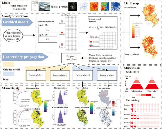
3.1. High-Resolution Gridded CO2 Emissions Map Patterns

3.1.1. High-Resolution Gridded CO2 Emissions Map

In this study, we used the gridded CO2 emissions maps constructed in previous studies [26,27,28]. Please see Tables S1–S3 (Supplementary Materials) for the composition and the heterogeneity analysis of the maps. The annual CO2 emissions per capita of Jinjiang city was 8.12 t in 2013, and 10,000 yuan of Jinjiang’s GDP caused 1.219 t of CO2 emissions. The total emission patterns of the 30 m and 500 m resolution CO2 emissions maps were similar (Figure 2a,e). The highest CO2 emission grids were located in the urban residential areas in the northern region, and in the industrial areas in the central region. Rural areas had low values of CO2 emissions. Residential emissions were concentrated in the northern built-up area, with high values of CO2 emissions being observed on the 500 m resolution map in this built-up area (Figure 2b,f). The distribution of industrial emissions was wider and more fragmented on the 500 m resolution map than on the 30 m resolution map (Figure 2c,g). Transport CO2 emissions were clearly distributed along roads on both maps (Figure 2d,h).

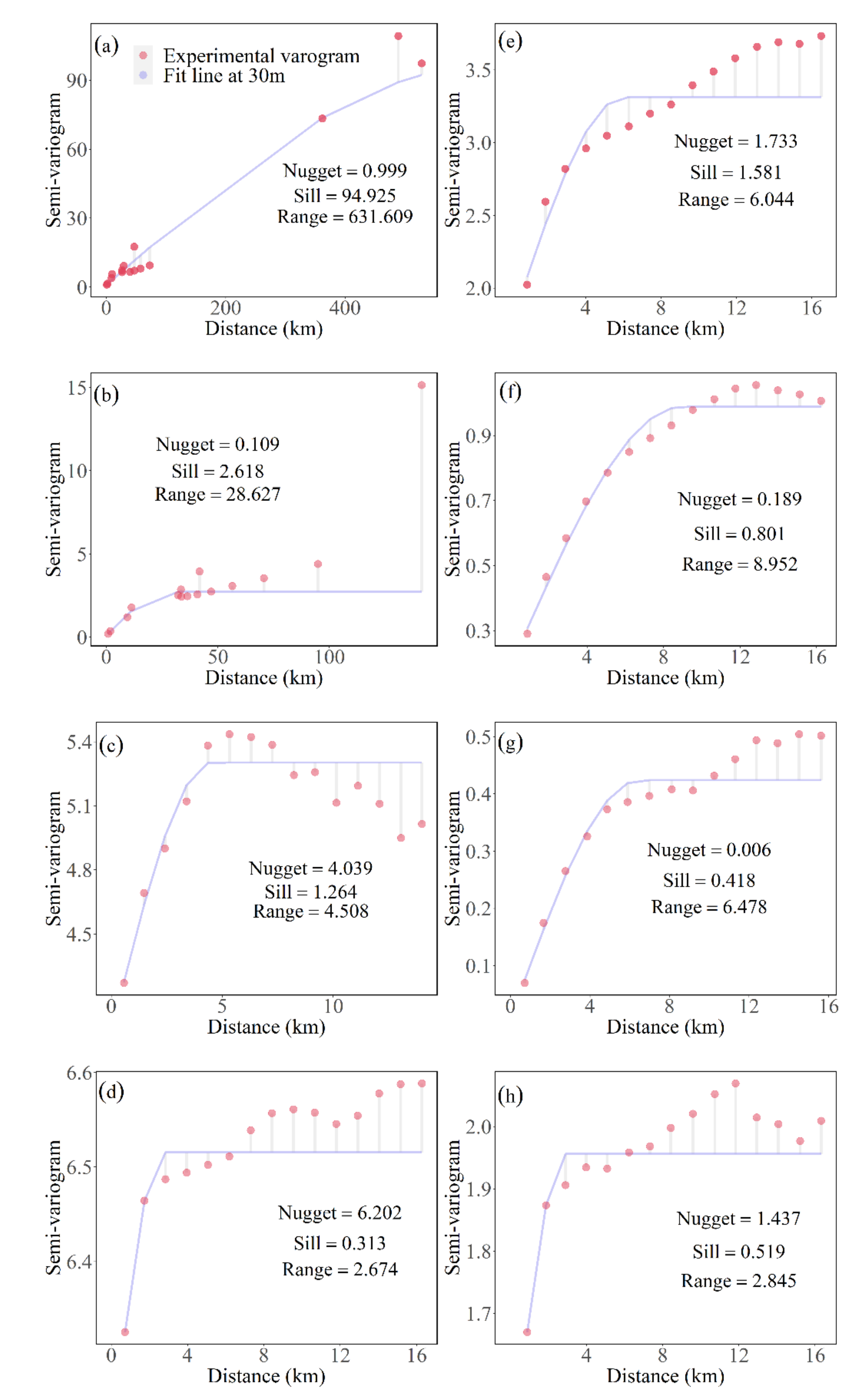
3.1.2. Spatial Variation of CO2 Emissions

We constructed semi-variograms of CO2 emissions to understand their spatial variation [32] (Figure 3); detailed information of the method is shown in the Supplementary Materials. The well-known geo-statistical concepts of nugget and sill represent the values at which the semi-variogram almost intercepts the y-value, and the values at which the model first flattens out, respectively [33]. The greater the sum of nugget and sill, the larger the spatial variation of CO2 emissions [34]. The results indicate that the spatial variation of emissions was much larger at 30 m resolution than at 500 m resolution. At 30 m and 500 m resolution, the largest spatial variations were both recorded for transport emissions among the different sectors (Figure 3d,h).

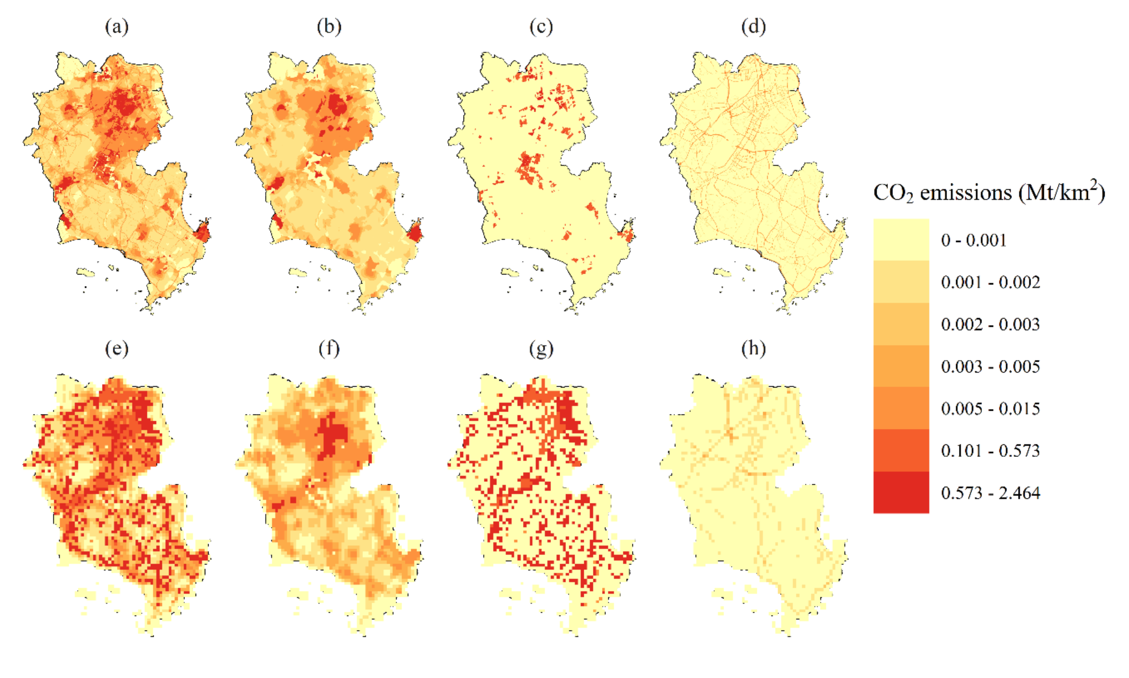
3.2. Propagated Uncertainties Caused by Gridded Model

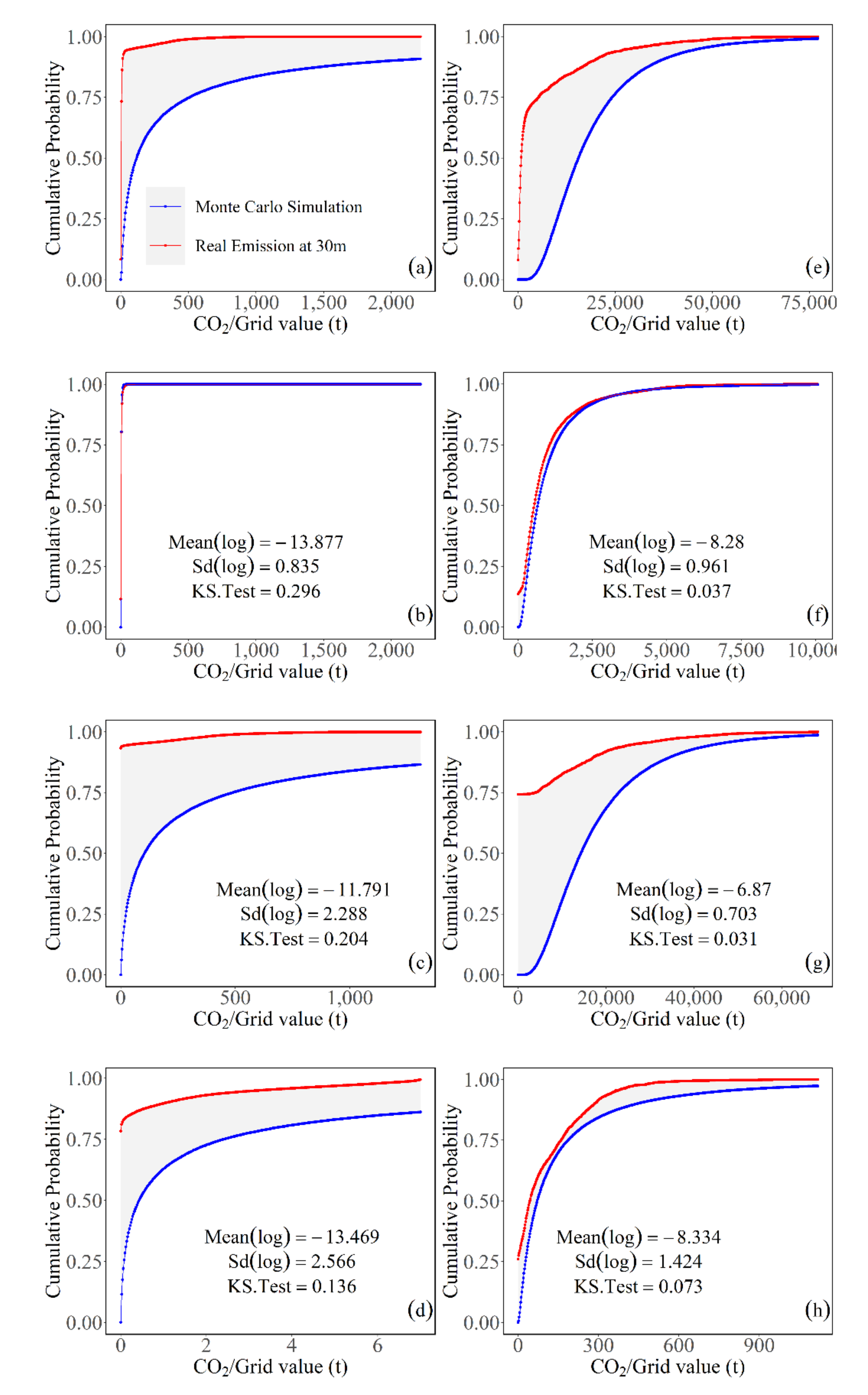
3.2.1. Results of the Uncertainty Estimation, Using U1

The logarithms of the mean and standard deviation of spatial proxies for CO2 emissions were obtained by fitting the PDFs (Figure 4). Smaller KS test values indicated better PDF fits. The KS test values of different maps and sectors were all less than 0.3, and were considered as good fits. The fitting performance of the 500 m resolution map was better than that of the 30 m resolution map. Based on the PDF fitting, we drew the curves of simulated and real CDFs for different resolutions (Figure 4). The CDFs represents the number (i.e., cumulative probability density) of each grid value occupied with the total number of grids. The CDF curve is an ascending order by x value. Hence, the cumulative probability density of a larger x value is almost 1. The uncertainty was the area between the two curves (gray area in Figure 4). The uncertainty of any pixel value was the difference between the y coordinates of the two curves when the pixel value was the corresponding x value. Comparison of the CDF curves of simulated emissions with actual emissions (Figure 4) showed that the uncertainty of the residential emissions was the smallest, while that of transport emissions was slightly larger, and that of industrial emissions was the largest. Overall, the uncertainty in the 500 m resolution map was smaller, and tended to decrease as CO2 emissions increased. In comparison, the uncertainty in 30 m CO2 emissions showed no significant change as CO2 emissions increased. When comparing the different sectors, there was less uncertainty regarding residential emissions in both the 30 m and 500 m resolution maps, which was represented by the coincident two color curves (Figure 4b,f). Uncertainty in industrial emissions was very large (up to nearly 80%) at 20,000 t/pixel, but it gradually decreased, and stayed within 10% beyond 20,000 t. The uncertainty on the 30 m map was almost always maintained at about 40% (Figure 4c,g). When the transport discharge pixel value was between 300 and 600 t, the uncertainty was small, but then gradually decreased with increasing pixel values on the 500 m map. There was always about 30% uncertainty in the 30 m map (Figure 4d,h).
The uncertainty map for the gridded model was generated by a look-up table (Figure 5). Among the uncertainty maps of total and industrial CO2 emissions (Figure 5a,c,e,g), the number of grids whose uncertainty reached 100% accounted for more than 80% of the area. However, most of the corresponding CO2 emissions of these grids were equal to zero. Most grids below 100% located in the residential and industrial areas of Jinjiang city. For the uncertainty maps of residential CO2 emissions (Figure 5b,f), almost half of the grids of the 30 m resolution uncertainty maps have low uncertainty (i.e., the average value of the uncertainty grids was 0.969%). With the other resolution map, most uncertainty grids were less than 25%. For the uncertainty maps of transport CO2 emissions (Figure 5d,h), most non-100% uncertainty grids were distributed along the roads. Compared with the 500 m resolution uncertainty map, the 30 m resolution uncertainty map had more 100% uncertainty grids. Furthermore, other grids of the 30 m and 500 m resolution uncertainty maps were below 50%.

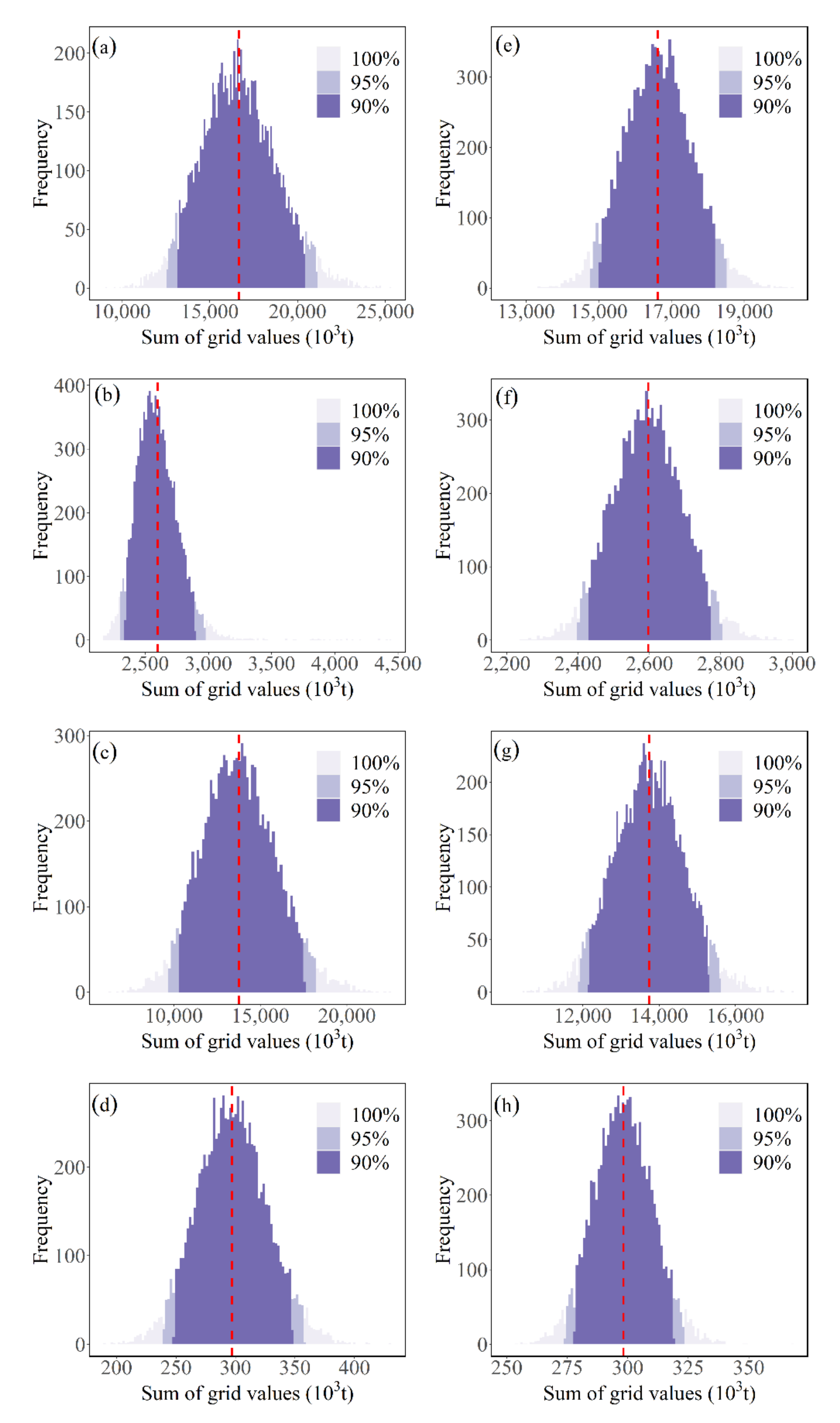
3.2.2. Results of the Uncertainty Estimation Using U2

The statistical terms and population distributions (sums of the grid values) were obtained based on the bootstrap sampling method described in the methods section. Then, the uncertainties and CIs were calculated (Figure 6, Table 1), the smallest uncertainty was obtained for residential emissions (12.84% and 7.68%), while CO2 emissions from industry remained the main source of uncertainty. Transport emissions were relatively small, with a small uncertainty. The uncertainty of the 500 m resolution map was far less than that of the 30 m resolution map. Since the range of 95% CIs on the 500 m resolution map was much smaller than that on the 30 m resolution map, the estimated overall CO2 emissions of the 500 m resolution map were also closer to the calculated value. The relationship between the overall uncertainty of emissions and the uncertainty of the three sectors was not a simple linear superposition, with it presenting a nonlinear change, because the overall uncertainty was less than the sum of the uncertainty of the three sectors. The estimated total emissions were similar than the normal distribution based on 10,000 simulations (Figure 6). Only the estimates of residential emissions in the 30 m resolution map showed a right-skewed distribution (Figure 6b).

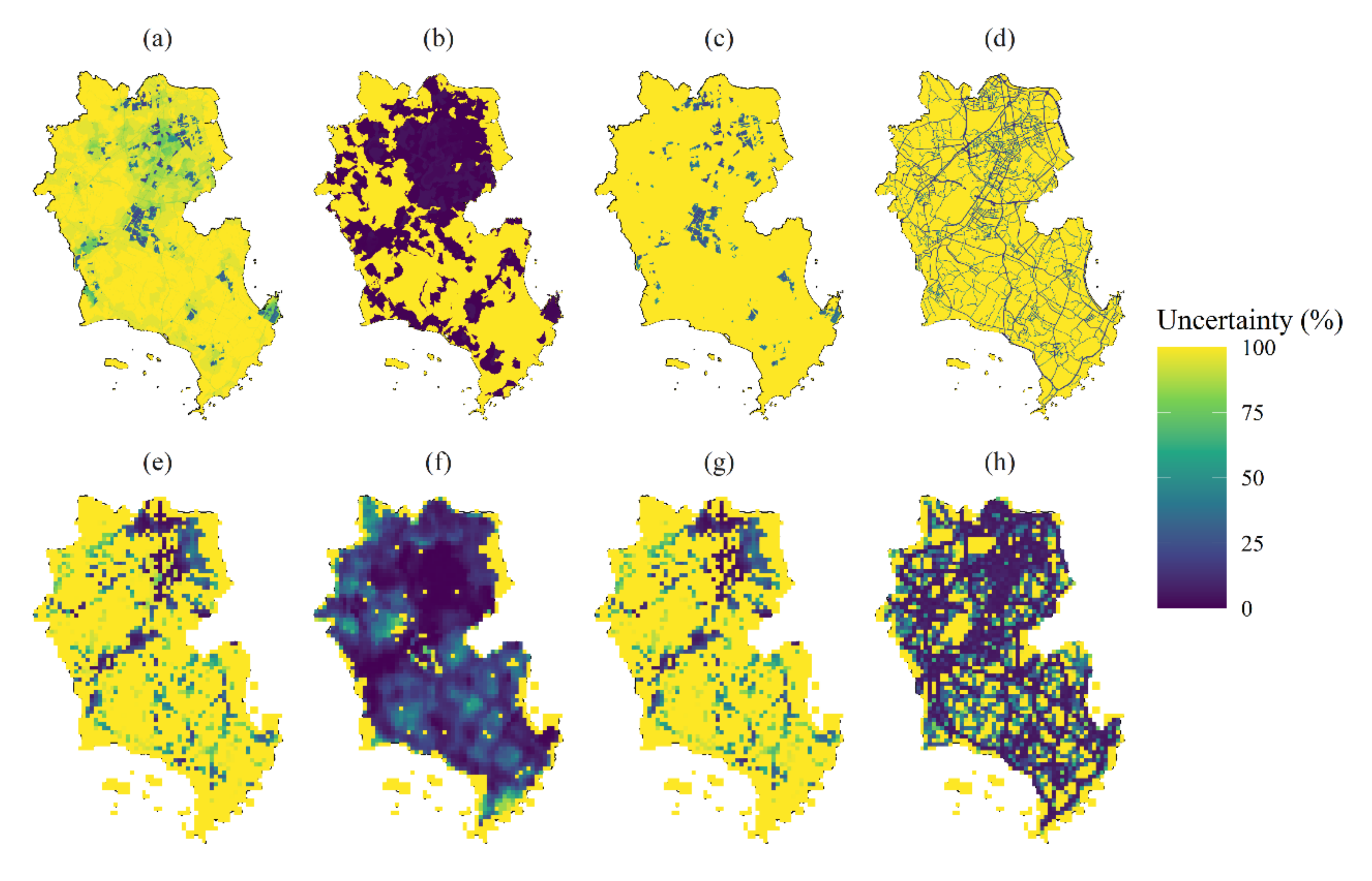
3.3. Propagated Uncertainties Caused by Input

3.3.1. Results of the Uncertainty Estimation Using U3

The constructed uncertainty maps for activity levels showed that the mean value of uncertainties for the grids of the 30 m resolution map was 37.30%, while that of the grids of the 500 m resolution map was 33.10%. The 95% CIs and uncertainty for residential, industrial, transport, and total activity levels were 1573 to 3594 (−39.13% ~ 39.08%), 11,005 to 16,424 (−19.81% ~ 19.67%), 205 to 392 (−31.25% ~ 31.59%), and 13,697 to 19,490 (−17.52% ~ 17.36%) thousand tons, and 39.11%, 19.74%, 31.42%, and 17.44%, respectively. The 95% CIs of the activity levels of the different emission types were within ±2σ. The 95% CIs of the total emissions were within ±20%, and had the lowest uncertainty compared to all of the sectors. The number of pixels with high uncertainty was greater in the 30 m resolution maps compared to the 500 m resolution maps (Figure 7). The uncertainties in the middle industrial areas and the northeastern built-up areas were smaller in both the 30 m and 500 m resolution maps (uncertainty was below 30%). Large areas with low uncertainty in the northern part of the 500 m resolution map had high uncertainty in the 30 m resolution map. Low uncertainty grids were scattered and fragmented in the 30 m resolution map (Figure 7a), but presented a continuous distribution in the 500 m resolution map (Figure 7b).

3.3.2. Results of the Uncertainty Estimation Using U4

U4 represents the uncertainty maps made with spatial proxies. The value of grids in the 30 m resolution map, which were regarded as the wrong grids, were generated by the product of average value of selected grids and a random error for residential, industrial, and transport emissions, were 19.85%, 20.00%, and 19.86%, respectively, while the total error was 33.67%. The errors in the spatial proxies of the distribution of residential, industrial, and transport emissions were 19.98%, 19.98%, and 19.98%, respectively, in the 500 m resolution map, while the total error was 24.35%. The overall error was greater than any initial error, and was less than the sum of the errors for the three sectors. The overall error presented a nonlinear change. The 500 m resolution map had less uncertainty than the 30 m resolution map. When there was a random error in spatial proxies, most areas overestimated emissions, with the errors of the urban areas and industrial areas with high emission intensity being large (Figure 8).

4. Discussion

4.1. Uncertainties

The process of mapping CO2 emissions is characterized by various uncertainties. Gurney [35] identified challenges in quantifying uncertainties in CO2 emissions, and suggested solutions, such as sensitivity testing of key inputs and parameters that are fully propagated through the estimation system. In this study, an analytic workflow inspired by the concept suggested by Gurney [35] was proposed to determine uncertainties at the urban scale.
Differences between estimations and actual emissions were generally used to measure the overall uncertainty in the estimation of emissions. Ou et al. [36] used relative error, mean relative error, and root mean square error to evaluate differences between actual and estimated data. This study used the CDF, which provided a description of the grid distribution features and allowed a comparison of the differences. The results indicated less uncertainty for residential emissions, which was in contrast to the uncertainties obtained from global mapping products. Andres et al. [21] analyzed uncertainty in three inputs of the CDIAC data product, and attributed 51% of the uncertainty to population data. Therefore, more accurate and detailed data were used to construct the population density gridded maps and reduce the uncertainties in this study. The results suggested that industrial emissions were the main uncertainty source in estimating urban CO2 emissions.
Several studies have investigated uncertainties caused by total CO2 emission estimations that are known to generate fundamental uncertainties [18,37]. Inventory accounting generates the quantities of total emissions that are eventually mapped. Since the uncertainties in activity levels and emission factors vary by sector and country, respectively, this study set the a priori uncertainty with normally distributed activity levels referenced by the paper of Zhao et al. (2012) [19]. Moreover, this study reported a greater, 95% CIs for total emissions than [19] did (−9 to 11%). The uncertainty estimated in this study (17.4%) was less than that determined from the CDIAC data for China (17.5%) [21]. These results could be attributed to the following reasons. First, this study focused on the propagation of uncertainty in activity levels during the gridding process. In contrast, Zhao et al. (2012) quantified uncertainty in the total CO2 emissions estimation of China through providing a detailed inventory while without quantifying uncertainties for the gridded process. Second, the trends for uncertainties in the total emissions and in the sums of emissions from different sectors were similar to those reported by Zhao et al. (2012) [19]. The uncertainty caused by the total emission estimations was significantly reduced by calculating the detailed inventories from different sectors, likely due to the “compensation of error” phenomenon that was realized through Monte Carlo simulations [19]. Finally, in contrast to Zhao et al. (2012), the higher uncertainty detected in this study could be attributed to the lack of detailed source categories. However, a comparison of results from the current study and the CDIAC indicated acceptable uncertainty levels.
Geospatial datasets were primarily used to obtain more accurate spatial proxies and reduce uncertainties in the gridded process. Uncertainties caused by spatial proxies also varied across different sectors. For instance, uncertainties in residential emissions were mainly attributed to errors in the generation of high-resolution population grids [21]. However, high population fitting accuracy at the street and town scales was generated in this study, and such spatial proxies of population were used to map residential emissions. Additionally, uncertainties in industrial emissions were mainly driven by the accuracy of industrial point-source data identification and the extent to which night time light intensity represented emissions intensity (saturation of bright lights [4]). Raupach et al. [38] indicated that correcting the saturation error of nighttime light imagery increased data values by 1.15–1.23 times, leading to greater uncertainty. Uncertainties in transport emissions existed, since road areas do not fully represent the intensity of CO2 emissions from traffic. Previous studies used traffic congestion conditions to calculate this parameter [39,40,41]. However, such data are difficult to acquire. Therefore, road area is generally used as a proxy in this research. Although road area is correlated with traffic jams and vehicle speed, it might not fully reflect traffic conditions [42].
In this study, data from the three sectors were ultimately spatially superimposed during the gridded process and represented the process of assigning spatial proxies. The U4 set 20% of the random errors in spatial proxies. Therefore, uncertainties caused by the total emission estimations were driven by the superimposition of interference from different sectors, were significantly less than 60%, and indicated a nonlinear increase. These results are supported by previous research on error transfer in cellular automaton models [43]. Yeh et al. [43] proposed that the errors in data sources did not propagate entirely to the final results. This means that the errors may be reduced after model processing, because their effects significantly decline during simulations. This argument is based on the assumption that the neighborhood calculation principle smooths errors. Therefore, the random error of total emissions was reduced by the compensation-of-error phenomenon, which is attributed to overlaying emissions from different sectors. Although the total quantity of emissions was stable for the whole city, errors increased at finer spatial resolutions. This finding is consistent with the results of Dong et al. [44], who mapped uncertainties in land use impacts on ecosystem services. Therefore, the impacts of spatial proxy errors on uncertainty were lower in coarse-resolution maps. This might be because fine-resolution maps have larger spatial variation in CO2 emissions than coarser-resolution maps. Dale et al. [45] attributed uncertainty in their model to an inadequate representation of spatial variability in natural elements. Spatial scale has been shown to significantly impact the spatial variation and distribution patterns of natural elements [46]. In this study, the fine-resolution map indicated higher spatial variation and larger uncertainty (Figure 3) than the coarse-resolution map. These results are supported by Ogle et al. [47], who reported that uncertainty was negatively correlated with spatial scale in their study on soil organic carbon. Cias et al. [48] analyzed uncertainty in CO2 emissions at the sub-national scale for 25 member states of the European Union, and concluded that uncertainty significantly increased when the resolution was smaller than 200 km. Therefore, multi-scale research is required to establish critical thresholds for scale selection [49,50,51].
The analytic workflow for uncertainty propagation proposed in this study may aid decision-makers in designing suitable low-risk policies. Regions with high emissions values and low uncertainties (industrial sources with emissions greater than 20,000 t/pixel and residential areas) could be the primary targets for emission reductions (Figure 4c). Therefore, the northern urban living areas and central regions could reduce emissions by promoting the development of low-carbon communities, and implementing energy-conservation and emission-reduction technologies. Furthermore, this study contributed to the research field of uncertainty analysis of urban scale CO2 emissions by proposing an analytic and reproducible workflow consisting of four submodules to investigate the uncertainty propagation during the gridding process caused by the gridded model and input. Previous studies used Monte Carlo simulation to estimate the uncertainty in CO2 emissions caused by inputs [10,11,12,15,52,53], the remaining studies used inventory comparison analysis to evaluate this uncertainty [5,25]. However, few studies considered the uncertainties caused by both the gridded model and the input. Furthermore, inventory comparison analysis is impossible at the urban scale due to the lack of a detailed emission inventory. The studies developed different uncertainty metrics and tools such as PDFs, the bootstrap sampling method, fuzzy mathematics, the 95% Cis, and relative uncertainty [54,55,56,57], which could provide the reference for our workflow. Moreover, some studies which retrieved CO2 emissions using atmospheric models used data assimilation technologies in an attempt to estimate and reduce the uncertainty in CO2 emissions [53,58]. These are novel technologies that can estimate the uncertainty but require complex atmospheric models and high-quality flux monitoring data. Compared with previous related studies, involving the construction and uncertainty propagation analysis of gridded maps of CO2 emissions, the workflow combined various methodologies of uncertainty analysis, including Monte Carlo simulation and the bootstrap sampling method, and enabled finding the completed uncertainties caused by the gridded model and input without detailed emission inventories, field measurements, or integration of complex atmospheric models.

4.2. Future Research Directions

Gridded CO2 emissions maps are likely to play an important role in climate change mitigation and sustainable development. Therefore, three future directions in this regard are proposed in the following sections based on a review of previous studies.
Advances in earth observation satellites and related technologies have enabled accurate, high-resolution quantification of CO2 emissions. Gridded CO2 emissions maps can be developed based on data obtained from night time light and greenhouse gas monitoring satellites [59,60,61]. However, relationships between night time light intensity and CO2 emissions are largely empirical [4,62]. Greenhouse gas monitoring satellites determine the actual concentrations of the CO2 column at low resolutions [63,64,65]. These limitations can be addressed by advances in earth observation satellites and implementation of novel technologies, including the development of satellites such as the LuoJia 1-01 and TanSAT [66,67,68]. However, limitations in estimating uncertainties in satellite-retrieved products still exist. The U4 which was developed in this study regarded a priori error of spatial input data or the quality assessment of satellite products as the uncertainty to estimate the uncertainties of gridded CO2 emissions maps. When we used remote sensing satellite products (such as MODIS-derived NDVI products) as input data, the satellite’s quality assessment files could be used to define a priori error, and to subsequently conduct uncertainty analyses [69].
The combination of carbon flux monitoring data and atmospheric models is essential for developing spatially explicit bottom-up CO2 emissions models. The bottom-up approach can estimate CO2 emissions with a high accuracy [22]. However, it requires high-quality and spatiotemporal resolution input data. For instance, the use of 14CO2 measurements can significantly assist the estimation of emissions from biological and fossil carbon pools [70,71,72]. Carbon flux monitoring data include anthropogenic and biogenic CO2 emissions [73]. However, long-term data on CO2 emissions and carbon fluxes are limited. Therefore, long-term carbon flux monitoring networks need to be established [74]. Although the Hestia and Anthropogenic Carbon Emissions System products have been used to develop spatially explicit CO2 emissions models, most data were obtained from the Indianapolis, Salt Lake City, Baltimore, and Los Angeles flux experiments [73]. However, such experiments are uncommon, and these studies coupled carbon flux monitoring data with atmospheric or chemistry transport models, such as the weather research and forecasting (WRF) model, the WRF model coupled with chemistry, the WRF Model coupled with the vegetation photosynthesis and respiration model, etc. [75,76]. Therefore, future studies (especially in China) should focus on different combinations of carbon flux monitoring data and atmospheric models.
Data assimilation technology allows the integration of satellite observation and model output data from atmospheric and oceanic models. Some studies have applied four-dimensional data assimilation of atmospheric CO2 using atmospheric infrared sounder observations [77]. However, studies focusing on data assimilation for CO2 emissions are limited because the coupled atmospheric model is difficult to construct and run. Moreover, there is a lack of satellite observations at a fine spatiotemporal resolution, and/or carbon flux monitoring data. The key components of data assimilation include observation data, uncertainty in observations, model outputs, uncertainty in model outputs, and data assimilation algorithms. Therefore, our workflow for uncertainty analysis is a powerful tool to aid data assimilation. Future research could focus on the integration of the present workflow with different data assimilation algorithms.

5. Conclusions

In this study, an analytic workflow was established to conduct uncertainty analyses. The workflow included four submodules which were used to evaluate the uncertainties which were propagated during the gridding process. The first and second submodules were designed to investigate the uncertainties of gridded CO2 emissions maps caused by the gridded model. The third and fourth submodules were used to analyze the uncertainties of the gridded CO2 emissions maps caused by the input. The results of our study demonstrated that different uncertainties were associated with the gridded process according to the statistical graph and gridded maps. Furthermore, we found that the uncertainties in the coarse-resolution map had a lower contribution to the uncertainties caused by the total emission estimations and spatial proxies. This may have been due to the fact that the fine-resolution map had a larger spatial variation in CO2 emissions. Furthermore, a nonlinear mapping relationship between the sum of the uncertainties of the gridded CO2 emissions maps among the different sectors and the final estimated uncertainties was found when the uncertainties of different sectors were spatially superimposed. This nonlinear relationship was attributed to the “compensation of error” phenomenon. That is, the overestimated and underestimated values among different sectors were offset at the same grid. In conclusion, this study provides the corresponding uncertainties of baseline data for developing low-carbon cities, as well as a general workflow for analyzing uncertainties in gridded CO2 emissions maps.

Supplementary Materials

The following are available online at https://www.mdpi.com/2072-4292/12/23/3932/s1, Table S1: CO2 emissions in Jinjiang city from different sectors in 2013; Table S2: Moran’s I for the different CO2 emissions sectors at different scales; Table S3 Factor detector q value of different CO2 emissions at different scales.

Author Contributions

Conceptualization, S.D. and S.Z.; methodology, S.D. and S.Z.; processing and analyses of data, C.L., J.L., and S.X.; visualization, S.D., writing-original draft preparation, S.D.; validation, B.C.; writing-review and editing, Y.R. All authors have read and agreed to the published version of the manuscript.

Funding

This work was supported by the National Science Foundation of China (42001210, 31670645, 31972951, 41801182, and 41807502), the National Social Science Fund (17ZDA058), the Ningbo Municipal Department of Science and Technology (2019C10056), Fujian Provincial Department of S&T Project (2018T3018), the Strategic Priority Research Program of the Chinese Academy of Sciences (XDA23020502).

Conflicts of Interest

The authors declare no competing interests.

References

  1. Mi, Z.; Guan, D.; Liu, Z.; Liu, J.; Viguié, V.; Fromer, N.; Wang, Y. Cities: The core of climate change mitigation. J. Clean. Prod. 2019, 207, 582–589. [Google Scholar] [CrossRef]
  2. Gouldson, A.; Colenbrander, S.; Sudmant, A.; Papargyropoulou, E.; Kerr, N.; McAnulla, F.; Hall, S. Cities and climate change mitigation: Economic opportunities and governance challenges in Asia. Cities 2016, 54, 11–19. [Google Scholar] [CrossRef] [Green Version]
  3. Gurney, K.R.; Romero-Lankao, P.; Seto, K.C.; Hutyra, L.R.; Duren, R.; Kennedy, C.; Grimm, N.B.; Ehleringer, J.R.; Marcotullio, P.; Hughes, S. Climate change: Track urban emissions on a human scale. Nature 2015, 525, 179. [Google Scholar] [CrossRef] [PubMed] [Green Version]
  4. Shi, K.; Chen, Y.; Yu, B.; Xu, T.; Chen, Z.; Liu, R.; Li, L.; Wu, J. Modeling spatiotemporal CO2 (carbon dioxide) emission dynamics in China from DMSP-OLS nighttime stable light data using panel data analysis. Appl. Energy 2016, 168, 523–533. [Google Scholar] [CrossRef]
  5. Gately, C.K.; Hutyra, L.R. Large Uncertainties in Urban-Scale Carbon Emissions. J. Geophys. Res. Atmos. 2017, 122, 211–242. [Google Scholar] [CrossRef]
  6. Gately, C.K.; Hutyra, L.R.; Sue Wing, I. Cities, traffic, and CO2: A multidecadal assessment of trends, drivers, and scaling relationships. Proc. Natl. Acad. Sci. USA 2015, 112, 4999. [Google Scholar] [CrossRef] [Green Version]
  7. City of New York. New York City’s Roadmap to 80 × 50; NYC Mayor’s Office of Sustainability: New York, NY, USA, 2016. [Google Scholar]
  8. Mi, Z.; Zhang, Y.; Guan, D.; Shan, Y.; Liu, Z.; Cong, R.; Yuan, X.C.; Wei, Y.M. Consumption-based emission accounting for Chinese cities. Appl. Energy 2016, 184, 1073–1081. [Google Scholar] [CrossRef] [Green Version]
  9. Su, W. Letter Including Autonomous Domestic Mitigation Actions. Appendix II—Nationally Appropriate Mitigation Actions of Developing Country Parties, United National Framework Convention on Climate Change. 2009, 11–14. Available online: http://unfccc.int/files/meetings/cop_15/copenhagen_accord/application/pdf/chinacphaccord_app2.pdf (accessed on 30 November 2020).
  10. Fang, C.; Wang, S.; Li, G. Changing urban forms and carbon dioxide emissions in China: A case study of 30 provincial capital cities. Appl. Energy 2015, 158, 519–531. [Google Scholar] [CrossRef]
  11. Wang, S.; Liu, X.; Zhou, C.; Hu, J.; Ou, J. Examining the impacts of socioeconomic factors, urban form, and transportation networks on CO2 emissions in China’s megacities. Appl. Energy 2017, 185, 189–200. [Google Scholar] [CrossRef]
  12. Wang, S.J.; Liu, X.P. China’s city-level energy-related CO2 emissions: Spatiotemporal patterns and driving forces. Appl. Energy 2017, 200, 204–214. [Google Scholar] [CrossRef]
  13. He, Z.; Xu, S.; Shen, W.; Long, R.; Chen, H. Impact of urbanization on energy related CO2 emission at different development levels: Regional difference in China based on panel estimation. J. Clean. Prod. 2017, 140, 1719–1730. [Google Scholar] [CrossRef]
  14. Wang, S.; Fang, C.; Guan, X.; Pang, B.; Ma, H. Urbanisation, energy consumption, and carbon dioxide emissions in China: A panel data analysis of China’s provinces. Appl. Energy 2014, 136, 738–749. [Google Scholar] [CrossRef]
  15. Shan, Y.; Guan, D.; Liu, J.; Mi, Z.; Liu, Z.; Liu, J.; Schroeder, H.; Cai, B.; Chen, Y.; Shao, S.; et al. Methodology and applications of city level CO2 emission accounts in China. J. Clean. Prod. 2017, 161, 1215–1225. [Google Scholar] [CrossRef] [Green Version]
  16. Shan, Y.; Liu, J.; Liu, Z.; Xu, X.; Shao, S.; Wang, P.; Guan, D. New provincial CO2 emission inventories in China based on apparent energy consumption data and updated emission factors. Appl. Energy 2016, 184, 742–750. [Google Scholar] [CrossRef] [Green Version]
  17. Liu, Z.; Guan, D.; Wei, W.; Davis, S.J.; Ciais, P.; Bai, J.; Peng, S.; Zhang, Q.; Hubacek, K.; Marland, G.; et al. Reduced carbon emission estimates from fossil fuel combustion and cement production in China. Nature 2015, 524, 335. [Google Scholar] [CrossRef] [Green Version]
  18. Wang, R.; Tao, S.; Ciais, P.; Shen, H.Z.; Huang, Y.; Chen, H.; Shen, G.F.; Wang, B.; Li, W.; Zhang, Y.Y.; et al. High-resolution mapping of combustion processes and implications for CO2 emissions. Atmos. Chem. Phys. 2013, 13, 5189–5203. [Google Scholar] [CrossRef] [Green Version]
  19. Zhao, Y.; Nielsen, C.P.; Mcelroy, M.B. China’s CO2 emissions estimated from the bottom up: Recent trends, spatial distributions, and quantification of uncertainties. Atmos. Environ. 2012, 59, 214–223. [Google Scholar] [CrossRef]
  20. Goodchild, M.F. Integrating Gis and Remote-Sensing for Vegetation and Analysis and Modeling—Methodological Issues. J. Veg. Sci. 1994, 5, 615–626. [Google Scholar] [CrossRef]
  21. Andres, R.J.; Boden, T.A.; Higdon, D.M. Gridded uncertainty in fossil fuel carbon dioxide emission maps, a CDIAC example. Atmos. Chem. Phys. 2016, 16, 14979–14995. [Google Scholar] [CrossRef] [Green Version]
  22. Gurney, K.R.; Liang, J.; O’Keeffe, D.; Patarasuk, R.; Hutchins, M.; Huang, J.; Rao, P.; Song, Y. Comparison of Global Downscaled Versus Bottom-Up Fossil Fuel CO2 Emissions at the Urban Scale in Four US Urban Areas. J. Geophys. Res. Atmos. 2019. [Google Scholar] [CrossRef]
  23. Andres, R.J.; Boden, T.A.; Breon, F.M.; Ciais, P.; Davis, S.; Erickson, D.; Gregg, J.S.; Jacobson, A.; Marland, G.; Miller, J.; et al. A synthesis of carbon dioxide emissions from fossil-fuel combustion. Biogeosciences 2012, 9, 1845–1871. [Google Scholar] [CrossRef] [Green Version]
  24. IPCC. Climate Change 2013: The Physical Science Basis; Cambridge University Press: Cambridge, UK; New York, NY, USA, 2013. [Google Scholar]
  25. Wang, M.; Cai, B. A two-level comparison of CO2 emission data in China: Evidence from three gridded data sources. J. Clean. Prod. 2017, 148, 194–201. [Google Scholar] [CrossRef]
  26. Dai, S.; Zuo, S.; Ren, Y. A spatial database of CO2 emissions, urban form fragmentation and city-scale effect related impact factors for the low carbon urban system in Jinjiang city, China. Data Brief 2020, 29, 105274. [Google Scholar] [CrossRef] [PubMed]
  27. Zuo, S.; Dai, S.; Ren, Y. More fragmentized urban form more CO2 emissions? A comprehensive relationship from the combination analysis across different scales. J. Clean. Prod. 2020, 244, 118659. [Google Scholar] [CrossRef]
  28. Dai, S.; Zuo, S.; Ren, Y. GISerDaiShaoqing/Urban-Carbon-Dioxide-Sources-Gridded-Maps-and-Its-Detemination-in-Jinjiang-City 0.4. 0.4 ed.; Zenodo: Genève, Switzerland, 2020. [Google Scholar] [CrossRef]
  29. Dai, S.; Zuo, S.; Ren, Y. High-resolution mapping of direct CO2 emissions and uncertainties at the urban scale. In Proceedings of the Spatial Accuracy 2018, Beijing, China, 21–25 May 2018; pp. 88–90. [Google Scholar]
  30. Stephens, M.A. EDF Statistics for Goodness of Fit and Some Comparisons. J. Am. Stat. Assoc. 1974, 69, 730–737. [Google Scholar] [CrossRef]
  31. Efron, B.; Tibshirani, R.J. An Introduction to the Bootstrap; Chapman & Hall: New York, NY, USA, 1994. [Google Scholar]
  32. Wu, J. Effects of changing scale on landscape pattern analysis: Scaling relations. Landsc. Ecol. 2004, 19, 125–138. [Google Scholar] [CrossRef]
  33. Cressie, N. Statistics for Spatial Data; John Wiley & Sons: Hoboken, NJ, USA, 2015. [Google Scholar]
  34. Chilès, J.P.; Delfiner, P. Geostatistics: Modeling Spatial Uncertainty; John Wiley & Sons: Hoboken, NJ, USA, 2012. [Google Scholar]
  35. Gurney, K.R. Recent research quantifying anthropogenic CO2 emissions at the street scale within the urban domain. Carbon Manag. 2014, 5, 309–320. [Google Scholar] [CrossRef]
  36. Ou, J.; Liu, X.; Li, X.; Shi, X. Mapping Global Fossil Fuel Combustion CO2 Emissions at High Resolution by Integrating Nightlight, Population Density, and Traffic Network Data. IEEE J. Sel. Top. Appl. 2016, 9, 1674–1684. [Google Scholar] [CrossRef]
  37. Bun, R.; Hamal, K.; Gusti, M.; Bun, A. Spatial GHG inventory at the regional level: Accounting for uncertainty. Clim. Chang. 2010, 103, 227–244. [Google Scholar] [CrossRef]
  38. Raupach, M.R.; Marland, G.; Ciais, P.; Le Quere, C.; Canadell, J.G.; Klepper, G.; Field, C.B. Global and regional drivers of accelerating CO2 emissions. Proc. Natl. Acad. Sci. USA 2007, 104, 10288–10293. [Google Scholar] [CrossRef] [Green Version]
  39. Chang, X.; Chen, B.Y.; Li, Q.; Cui, X.; Tang, L.; Liu, C. Estimating Real-Time Traffic Carbon Dioxide Emissions Based on Intelligent Transportation System Technologies. IEEE Trans. Intell. Transp. 2013, 14, 469–479. [Google Scholar] [CrossRef]
  40. Dang, Y.; Li, Y.; Sun, R.; Hu, B.; Zhang, T.; Liu, Y. Estimation of carbon dioxide emission in Beijing city. In 2009 Joint Urban Remote Sensing Event, Vols. 1–3; IEEE: Shanghai, China, 2009; pp. 1111–1116. [Google Scholar]
  41. Zhang, W.; Huang, B.; Luo, D. Effects of land use and transportation on carbon sources and carbon sinks: A case study in Shenzhen, China. Landsc. Urban Plan. 2014, 122, 175–185. [Google Scholar] [CrossRef]
  42. Shu, Y.; Lam, N.S.N. Spatial disaggregation of carbon dioxide emissions from road traffic based on multiple linear regression model. Atmos. Environ. 2011, 45, 634–640. [Google Scholar] [CrossRef]
  43. Yeh, A.G.O.; Li, X. Errors and uncertainties in urban cellular automata. Comput. Environ. Urban Syst. 2006, 30, 10–28. [Google Scholar] [CrossRef]
  44. Dong, M.; Bryan, B.A.; Connor, J.D.; Nolan, M.; Gao, L. Land use mapping error introduces strongly-localised, scale-dependent uncertainty into land use and ecosystem services modelling. Ecosyst. Serv. 2015, 15, 63–74. [Google Scholar] [CrossRef]
  45. Dale, V.H.; Jager, H.I.; Gardner, R.H.; Rosen, A.E. Using sensitivity and uncertainty analyses to improve predictions of broad-scale forest development. Ecol. Model. 1988, 42, 165–178. [Google Scholar] [CrossRef]
  46. Mearns, L.O.; Easterling, W.; Hays, C.; Marx, D. Comparison of Agricultural Impacts of Climate Change Calculated from High and Low Resolution Climate Change Scenarios: Part I. The Uncertainty Due to Spatial Scale. Clim. Chang. 2001, 51, 131–172. [Google Scholar] [CrossRef]
  47. Ogle, S.M.; Breidt, F.J.; Easter, M.; Williams, S.; Killian, K.; Paustian, K. Scale and uncertainty in modeled soil organic carbon stock changes for US croplands using a process-based model. Glob. Chang. Biol. 2010, 16, 810–822. [Google Scholar] [CrossRef]
  48. Ciais, P.; Paris, J.D.; Marland, G.; Peylin, P.; Piao, S.L.; Levin, I.; Pregger, T.; Scholz, Y.; Friedrich, R.; Rivier, L.; et al. The European carbon balance. Part 1: Fossil fuel emissions. Glob. Chang. Biol. 2010, 16, 1395–1408. [Google Scholar] [CrossRef]
  49. Greene, C.S.; Kedron, P.J. Beyond fractional coverage: A multilevel approach to analyzing the impact of urban tree canopy structure on surface urban heat islands. Appl. Geogr. 2018, 95, 45–53. [Google Scholar] [CrossRef]
  50. Li, C.; Li, J.; Wu, J. What drives urban growth in China? A multi-scale comparative analysis. Appl. Geogr. 2018, 98, 43–51. [Google Scholar] [CrossRef]
  51. Zhou, W.; Ming, D.; Lv, X.; Zhou, K.; Bao, H.; Hong, Z. SO–CNN based urban functional zone fine division with VHR remote sensing image. Remote Sens. Environ. 2020, 236, 111458. [Google Scholar] [CrossRef]
  52. Konovalov, I.B.; Berezin, E.V.; Ciais, P.; Broquet, G.; Beekmann, M.; Hadji-Lazaro, J.; Clerbaux, C.; Andreae, M.O.; Kaiser, J.W.; Schulze, E.D. Constraining CO2 emissions from open biomass burning by satellite observations of co-emitted species: A method and its application to wildfires in Siberia. Atmos. Chem. Phys. 2014, 14, 10383–10410. [Google Scholar] [CrossRef] [Green Version]
  53. Konovalov, I.B.; Berezin, E.V.; Ciais, P.; Broquet, G.; Zhuravlev, R.V.; Janssens-Maenhout, G. Estimation of fossil-fuel CO2 emissions using satellite measurements of “proxy” species. Atmos. Chem. Phys. 2016, 16, 13509–13540. [Google Scholar] [CrossRef] [Green Version]
  54. Cao, Z.; Shen, L.; Zhao, J.; Liu, L.; Zhong, S.; Sun, Y.; Yang, Y. Toward a better practice for estimating the CO2 emission factors of cement production: An experience from China. J. Clean. Prod. 2016, 139, 527–539. [Google Scholar] [CrossRef]
  55. Lu, W.T.; Dai, C.; Fu, Z.H.; Liang, Z.Y.; Guo, H.C. An interval-fuzzy possibilistic programming model to optimize China energy management system with CO2 emission constraint. Energy 2018, 142, 1023–1039. [Google Scholar] [CrossRef]
  56. Su, X.; Shiogama, H.; Tanaka, K.; Fujimori, S.; Hasegawa, T.; Hijioka, Y.; Takahashi, K.; Liu, J. How do climate-related uncertainties influence 2 and 1.5 °C pathways? Sustain. Sci. 2018, 13, 291–299. [Google Scholar] [CrossRef] [Green Version]
  57. Carotenuto, F.; Gualtieri, G.; Miglietta, F.; Riccio, A.; Toscano, P.; Wohlfahrt, G.; Gioli, B. Industrial point source CO2 emission strength estimation with aircraft measurements and dispersion modelling. Environ. Monit. Assess. 2018, 190, 165. [Google Scholar] [CrossRef] [Green Version]
  58. Lauvaux, T.; Miles, N.L.; Deng, A.; Richardson, S.J.; Cambaliza, M.O.; Davis, K.J.; Gaudet, B.; Gurney, K.R.; Huang, J.; O’Keefe, D.; et al. High-resolution atmospheric inversion of urban CO2 emissions during the dormant season of the Indianapolis Flux Experiment (INFLUX). J. Geophys. Res. Atmos. 2016, 121, 5213–5236. [Google Scholar] [CrossRef] [Green Version]
  59. Doll, C.N.H.; Muller, J.P.; Elvidge, C.D. Night-time imagery as a tool for global mapping of socioeconomic parameters and greenhouse gas emissions. Ambio J. Hum. Environ. 2000, 29, 157–162. [Google Scholar] [CrossRef]
  60. Liang, A.; Gong, W.; Han, G.; Xiang, C. Comparison of Satellite-Observed XCO2 from GOSAT, OCO-2, and Ground-Based TCCON. Remote Sens. 2017, 9, 1033. [Google Scholar] [CrossRef] [Green Version]
  61. Shi, K.; Chen, Y.; Li, L.; Huang, C. Spatiotemporal variations of urban CO2 emissions in China: A multiscale perspective. Appl. Energy 2018, 211, 218–229. [Google Scholar] [CrossRef]
  62. Meng, L.; Graus, W.; Worrell, E.; Huang, B. Estimating CO2 (carbon dioxide) emissions at urban scales by DMSP/OLS (Defense Meteorological Satellite Program’s Operational Linescan System) nighttime light imagery: Methodological challenges and a case study for China. Energy 2014, 71, 468–478. [Google Scholar] [CrossRef]
  63. Hammerling, D.M.; Michalak, A.M.; Kawa, S.R. Mapping of CO2 at high spatiotemporal resolution using satellite observations: Global distributions from OCO-2. J. Geophys. Res. Atmos. 2012, 117. [Google Scholar] [CrossRef]
  64. Hammerling, D.M.; Michalak, A.M.; O’Dell, C.; Kawa, S.R. Global CO2 distributions over land from the Greenhouse Gases Observing Satellite (GOSAT). Geophys. Res. Lett. 2012, 39. [Google Scholar] [CrossRef] [Green Version]
  65. Zeng, Z.C.; Lei, L.; Strong, K.; Jones, D.B.A.; Guo, L.; Liu, M.; Deng, F.; Deutscher, N.M.; Dubey, M.K.; Griffith, D.W.T.; et al. Global land mapping of satellite-observed CO2 total columns using spatio-temporal geostatistics. Int. J. Digit. Earth 2017, 10, 426–456. [Google Scholar] [CrossRef] [Green Version]
  66. Jiang, W.; He, G.; Long, T.; Guo, H.; Yin, R.; Leng, W.; Liu, H.; Wang, G. Potentiality of Using Luojia 1-01 Nighttime Light Imagery to Investigate Artificial Light Pollution. Sensors 2018, 18, 2900. [Google Scholar] [CrossRef] [Green Version]
  67. Li, X.; Zhao, L.; Li, D.; Xu, H. Mapping Urban Extent Using Luojia 1-01 Nighttime Light Imagery. Sensors 2018, 18, 3665. [Google Scholar] [CrossRef] [Green Version]
  68. Yang, D.; Liu, Y.; Cai, Z.; Chen, X.; Yao, L.; Lu, D. First Global Carbon Dioxide Maps Produced from TanSat Measurements. Adv. Atmos. Sci. 2018, 35, 621–623. [Google Scholar] [CrossRef]
  69. Gu, J.; Li, X.; Huang, C.; Okin, G.S. A simplified data assimilation method for reconstructing time-series MODIS NDVI data. Adv. Space Res. 2009, 44, 501–509. [Google Scholar] [CrossRef]
  70. Gurney, K.R.; Liang, J.; Patarasuk, R.; O’Keeffe, D.; Huang, J.; Hutchins, M.; Lauvaux, T.; Turnbull, J.C.; Shepson, P.B. Reconciling the differences between a bottom-up and inverse-estimated FFCO 2 emissions estimate in a large US urban area. Elem. Sci. Anth. 2017, 5. [Google Scholar] [CrossRef] [Green Version]
  71. Turnbull, J.C.; Miller, J.B.; Lehman, S.J.; Tans, P.P.; Sparks, R.J.; Southon, J. Comparison of 14CO2, CO, and SF6 as tracers for recently added fossil fuel CO2 in the atmosphere and implications for biological CO2 exchange. Geophys. Res. Lett. 2006, 33. [Google Scholar] [CrossRef]
  72. Miller, J.B.; Lehman, S.J.; Montzka, S.A.; Sweeney, C.; Miller, B.R.; Karion, A.; Wolak, C.; Dlugokencky, E.J.; Southon, J.; Turnbull, J.C.; et al. Linking emissions of fossil fuel CO2 and other anthropogenic trace gases using atmospheric 14CO2. J. Geophys. Res. Atmos. 2012, 117. [Google Scholar] [CrossRef]
  73. Turnbull, J.C.; Karion, A.; Davis, K.J.; Lauvaux, T.; Miles, N.L.; Richardson, S.J.; Sweeney, C.; McKain, K.; Lehman, S.J.; Gurney, K.R. Synthesis of Urban CO2 Emission Estimates from Multiple Methods from the Indianapolis Flux Project (INFLUX). Environ. Sci. Technol. 2018, 53, 287–295. [Google Scholar] [CrossRef]
  74. Mitchell, L.E.; Lin, J.C.; Bowling, D.R.; Pataki, D.E.; Strong, C.; Schauer, A.J.; Bares, R.; Bush, S.E.; Stephens, B.B.; Mendoza, D.; et al. Long-term urban carbon dioxide observations reveal spatial and temporal dynamics related to urban characteristics and growth. Proc. Natl. Acad. Sci. USA 2018, 115, 2912. [Google Scholar] [CrossRef] [Green Version]
  75. Park, C.; Gerbig, C.; Newman, S.; Ahmadov, R.; Feng, S.; Gurney, K.R.; Carmichael, G.R.; Park, S.Y.; Lee, H.W.; Goulden, M.; et al. CO2 Transport, Variability, and Budget over the Southern California Air Basin Using the High-Resolution WRF-VPRM Model during the CalNex 2010 Campaign. J. Appl. Meteorol. Climatol. 2018, 57, 1337–1352. [Google Scholar] [CrossRef]
  76. INFLUX. Indianapolis Flux Experiment (INFLUX). Available online: https://sites.psu.edu/influx/publications/ (accessed on 13 November 2020).
  77. Engelen, R.J.; Serrar, S.; Chevallier, F. Four-dimensional data assimilation of atmospheric CO2 using AIRS observations. J. Geophys. Res. Atmos. 2009, 114. [Google Scholar] [CrossRef]
Figure 1. Analytic workflow of the uncertainty propagation in gridded CO2 emission maps. ALs, activity levels; CI, confidence interval; EFs, emission factors; GDP, gross domestic product; KS, Kolmogorov–Smirnov; LUT, look up table; MLE, maximum likelihood estimation; NTL, night time light; PDFs, probability distribution functions.
Remotesensing 12 03932 g001
Figure 2. Maps showing CO2 emissions in Jinjiang city at resolutions of 30 m (ad) and 500 m (eh). (a,e) show total CO2 emissions. (b,f) show residential CO2 emissions. (c,g) show industrial CO2 emissions. (d,h) show transport CO2 emissions.
Remotesensing 12 03932 g002
Figure 3. Semi-variograms of different sources of CO2 emissions from the 30 m resolution maps (ad) and the 500 m resolution maps (eh). (a,e) show total CO2 emissions. (b,f) show residential CO2 emissions. (c,g) show industrial CO2 emissions. (d,h) show traffic CO2 emissions.
Remotesensing 12 03932 g003
Figure 4. CDF curve of different CO2 emissions at 30 m and 500 m resolution. The upper figures are at 30 m resolution, while the lower figures are at 500 m resolution. The red line is the distribution of the real values, while the blue line is the distribution of the simulated values. (a,e) are the total CO2 emissions, (b,f) are the residential CO2 emissions, (c,g) are the industrial CO2 emissions, and (d,h) are the transport CO2 emissions. KS., Kolmogorov–Smirnov; Sd, Standard deviation.
Remotesensing 12 03932 g004
Figure 5. Uncertainty maps made by the gridded model of CO2 emissions in Jinjiang city, at resolutions of 30 m (ad) and 500 m (eh). (a,e) show uncertainty maps of total CO2 emissions. (b,f) show uncertainty maps of residential CO2 emissions. (c,g) show uncertainty maps of industrial CO2 emissions. (d,h) show uncertainty maps of transport CO2 emissions.
Remotesensing 12 03932 g005
Figure 6. CO2 emission population (statistic term) distributions of different sectors. The left figures are at 30 m resolution, while the right figures are at 500 m resolution. The red line is the distribution of the real values, and the blue line is the distribution of the simulated values. (a,e) are the total CO2 emissions, (b,f) are the residential CO2 emissions, (c,g) are the industrial CO2 emissions, and (d,h) are the transport CO2 emission.
Remotesensing 12 03932 g006
Figure 7. Map showing the uncertainty caused by activity levels. (a,b) represent the uncertainty maps of total CO2 emissions at 30 m and 500 m resolution, respectively.
Remotesensing 12 03932 g007
Figure 8. Maps of uncertainty caused by the spatial proxies. (a,b) represent the maps of uncertainty of total CO2 emissions at 30 m and 500 m resolutions.
Remotesensing 12 03932 g008
Table 1. Uncertainty in CO2 emissions (x 103 t) from different sectors from the 30 m and 500 m resolution maps.
Source95 CI (Range %)MeanUncertainty
30 m500 m30 m500 m30 m500 m
Residential2304 to 2970
(−11% to +14%)
2401 to 2799
(−8% to +8%)
2596259612.84%7.68%
Industrial9744 to 18,170
(−29% to +32%)
11,917 to 15,591
(−13% to +14%)
13,75913,73130.62%13.38%
Transport240 to 357
(−19% to +20%)
274 to 323
(−8% to +8%)
29729819.67%8.19%
Total12,289 to 21,498
(−26% to +29%)
14,593 to 18,714
(−12% to +13%)
16,65316,62427.65%12.40%
Notes: the uncertainty is equal to the mean value of CO2 emissions for the selected grid in the bootstrap sampling method divided by the 95% CIs width of CO2 emissions at the selected grid in the bootstrap sampling method. CI, confidence interval.
Publisher’s Note: MDPI stays neutral with regard to jurisdictional claims in published maps and institutional affiliations.

