Remotely Sensed Mid-Channel Bar Dynamics in Downstream of the Three Gorges Dam, China


1
Key Laboratory of Reservoir Aquatic Environment, Chongqing Institute of Green and Intelligent Technology, Chinese Academy of Sciences, Chongqing 400714, China
2
Department of Forestry and Natural Resources, Purdue University, West Lafayette, IN 47906, USA
3
State Key Laboratory of Lake Science and Environment, Nanjing Institute of Geography and Limnology, Chinese Academy of Sciences, 73 East Beijing Road, Nanjing 210008, China
4
Department of Geography and Environmental Science, University of Reading, Whiteknights, Reading RG6 6AB, UK
5
Lancaster Environment Centre, Lancaster University, Lancaster LA1 4YQ, UK
*
Author to whom correspondence should be addressed.
Remote Sens. 2020, 12(3), 409; https://doi.org/10.3390/rs12030409
Submission received: 27 December 2019
/
Revised: 21 January 2020
/
Accepted: 25 January 2020
/
Published: 28 January 2020
(This article belongs to the Special Issue Advancements in Remote Sensing of Land Surface Change)
Abstract
:The downstream reach of the Three Gorges Dam (TGD) along the Yangtze River (1560 km) hosts numerous mid-channel bars (MCBs). MCBs dynamics are crucial to the river’s hydrological processes and local ecological function. However, a systematic understanding of such dynamics and their linkage to TGD remains largely unknown. Using Landsat-image-extracted MCBs and several spatial-temporal analysis methods, this study presents a comprehensive understanding of MCB dynamics in terms of number, area, and shape, over downstream of TGD during the period 1985–2018. On average, a total of 140 MCBs were detected and grouped into four types representing small (<2 km2), middle (2 km2 – 7 km2), large (7 km2 – 33 km2) and extra-large size (>33 km2) MCBs, respectively. MCBs number decreased after TGD closure but most of these happened in the lower reach. The area of total MCBs experienced an increasing trend (2.77 km2/yr, p-value < 0.01) over the last three decades. The extra-large MCBs gained the largest area increasing rate than the other sizes of MCBs. Small MCBs tended to become relatively round, whereas the others became elongate in shape after TGD operation. Impacts of TGD operation generally diminished in the longitudinal direction from TGD to Hankou and from TGD to Jiujiang for shape and area dynamics, respectively. The quantified longitudinal and temporal dynamics of MCBs across the entire Yangtze River downstream of TGD provides a crucial monitoring basis for continuous investigation of the changing mechanisms affecting the morphology of the Yangtze River system.
1. Introduction
Most large rivers in the world are strongly regulated and engineered by artificial facilities [1]. The most common facilities are dams, as they lead to discontinuity and alteration in the hydrological and ecological processes of river systems [2,3]. Accordingly, increasing attention has been paid to the various impacts of damming on the hydrological and ecological processes of downstream systems, such as the morphodynamics of river channel forms [4,5]. One type of channel form that is potentially affected by damming is the mid-channel bar (MCB), also known as river island (i.e., an elevated region surrounded by river water) [6,7]. As an essential geomorphic unit and component in a fluvial system, MCBs directly influence a river’s morphological evolution and sediment archiving through their interaction with the flow and sediment transport [8,9,10,11]. Therefore, MCB dynamics in the context of damming intervention are especially important in maintaining the stability of river channels [12] and ecosystem functions (e.g., biodiversity and habitat providing) of the related hydro-ecosystems [13,14].
Under natural river regimes, MCBs often experience predictable geomorphic evolution in terms of area, shape, height, and location, due to longitudinal and temporal variations in flow and sediment load [15,16]. With intensive human interventions such as dam operation, natural river regimes are gradually replaced by regulated flow and sediment load, which dramatically affects the MCBs’ evolution processes and thereby creates scientific and social concerns internationally [10,17,18]. For example, the dynamics of MCBs together with the changes of dam-induced channel hydrologic regime have been examined in large rivers across the globe, such as the UK [19], Australia [20], the USA [21], France [22], and China [23]. It is crucial to explore the longitudinal and temporal dynamics of MCBs to reveal the response of bar development to the associated impact factors (e.g., damming, water flow, sediment load, and boundary conditions) and, eventually, to project the MCB evolution in the future scenarios [11,24]. Therefore, understanding MCB dynamics is important not only for developing geomorphic theory but also for informing hydraulic engineering practices on rivers, particularly in large rivers that experience extensive anthropogenic influences [6,10].
As the largest river in China, the Yangtze River plays a key role in maintaining ecological security (e.g., wetland protection, fishing management, and shoreline protection) and economic development (e.g., shipping, sand supply, and land development) [25]. This is especially true for the downstream reach of the three gorges dam (TGD) on the Yangtze River as it passes through one of the country’s most densely populated and most industrialized regions [26,27]. Historically, the MCBs in the mid-lower reach of the Yangtze River (i.e., downstream of TGD) are considered important land resources for channel dredging, habitat, and even agricultural development and urbanization, depending on the sizes and geographical conditions (e.g., stability, vegetation, and soil) [12]. Over the past three decades, the hydrodynamics in this reach, however, experienced extensive changes due to various anthropogenic activities, such as the construction of TGD [28]. By considering such massive environmental alterations and the ecological importance of the MCBs, two important questions have been raised: (1) How did MCB dynamics differ between the pre- and post-dam periods? (2) To what extent were they influenced by the dam?
Many previous investigations of the MCB dynamics with respect to damming or reservoir construction have been made over the last five decades. Petts [19] reviewed potential bar dynamics subsequent to dams along multiple British rivers. These earlier investigations were focused more on geomorphologic theory, such as the description of development stages (e.g., formation, migration, translation, and channel equilibrium) through experimental work or field studies, but within a limited longitudinal-temporal span [9]. Since the 1980s, research on MCB dynamics in the context of large scale and long-term temporal span, however, received increasingly wider attention [10,15], thanks to the rapid development of Remote Sensing (RS) technology and the sophisticated requirements for river regulation [29,30]. Among these studies, the common observations are that the area and number of MCBs tend to decrease due to the dam-induced sediment supply reduction [1,23,31]. In other cases, however, different patterns have been observed. In the Missouri River, Sanford [32] showed that the dam-regulated flow caused a series of consequences on bars, such as area reduction, less bar migrations, and more bar aggregation. Kiss and Balogh [33] showed that MCBs developed quickly in the upstream and laterally in the whole section of the Dráva River because of the coarse sediment supply and the decreasing stream energy due to the dam. These findings suggest that the downstream geomorphic adjustments to dam operations could result in different types of MCB dynamics (e.g., emergence, stability, or erosion), which depends upon the new hydraulic regime, sediment supply, and the type of structures employed [1,34].
Since the closure of TGD, the effects of dramatic dam operation on its downstream reaches have been discussed extensively. Most of the topics are focused on flow and sediment regime changes and channel morphology dynamics [17,35,36]. However, only a few studies analyzed the MCB dynamics at a large spatiotemporal scale with the help of RS technology [12,23,30,37]. For example, in the reach immediately downstream of TGD, Wang et al. [23] found that the total area of MCBs extracted from Landsat images reduced dramatically by 19.23% from 2003 to 2016, accompanied with an increase of water surface width. Lou et al. [12] focused on the lower reach and found the MCBs’ total area exhibited a decreasing trend in the pre-TGD period, but an increasing trend in the post-TGD period. It is noted that these results were based only on the area metric of large MCB in a limited reach. Such results are too limited to support a systematic understanding of the MCB dynamics over the entire Yangtze River downstream of TGD.
This work, therefore, made the attempted to comprehensively analyze the MCBs dynamics over the entire Yangtze River downstream of TGD throughout the last three decades (covering pre-TGD and post-TGD periods), by (1) inventorying MCBs extracted from time-series satellite imagery and (2) understanding the spatial (or longitudinal) and temporal patterns of the MCBs under the local damming and other anthropogenic contexts with three morphology-related metrics: MCB number, area, and shape.
2. Materials and Methods
2.1. Study Area
The Yangtze River originates on the Qinghai-Tibet Plateau 5100 m above sea level and flows eastward to the East China Sea. It is the largest river on the Eurasian continent and third longest river in the world, with a length of 6300 km and a drainage area of about 1.8 × 10⁶ km2. The climate is controlled by the East Asian Monsoon with the basin-wide precipitation averages around 1100 mm/yr [38]. The mainstream of the Yangtze River consists of the three reaches (Figure 1): the upper reach from the head to Yichang (YC), the middle reach from YC to Hankou (HK), and the lower reach from HK to the estuary (EST) near Shanghai City. TGD lies 43 km upstream of YC (Figure 1). It is the largest hydropower dam in the world. TGD was closed in 2003 and has been fully operational since 2010. The general principle guiding TGD operation is to keep the water level of the Three Gorges Reservoir (TGR) at the lowest (to 145 m) in flood season from May to September and at the highest (to 175 m) in dry season from October to April in the following year [39]. Accordingly, the hydrological and sediment regimes in the downstream of TGD are altered [24].
The downstream reach of TGD served as our study area (Figure 1). It is 1560 km long and consists of both middle and lower reaches of the Yangtze River. Its channel is much wider (from 900 m to 1800 m) and the river’s slope is smaller (with an average slope of 0.0256‰) than these in the upstream of TGD. Surrounding the channel is one of China’s most densely populated and highly industrialized regions [39]. Thus, apart from hydrology alteration by TGD operation, the downstream reach of TGD is also affected by various human activities, such as navigation, sand mining, agricultural activities, and urbanization. Moreover, the ecological values of this reach have been highly recognized, such as wetland protection, rare animal protection, and ecological sustainability maintenance [40].
2.2. Data Sources
2.2.1. Landsat Images
The free Landsat archive images obtained from 1985 to 2018 were used as raw image sources for extracting long-term MCB datasets. They include Landsat -4/5 TM (1985–2011), -7 ETM+ SLC-ON (1999–2003), -7 ETM+ SLC-OFF (2009–2012), and -8 OLI images (2013–2018). All the images are standard Landsat surface reflectance level-2 products with 30 m spatial resolution. They were ordered from the United States Geological Survey (USGS)’s Earth Explorer (http://earthexplorer.usgs.gov/) and downloaded from the USGS’s Earth Resources Observation and Science Center Science Processing Architecture on Demand Interface (https://espa.cr.usgs.gov/). Landsat-4/5 TM and Landsat-7 ETM+ surface reflectance data were produced by the software of Landsat Ecosystem Disturbance Adaptive Processing System (LEDAPS) [41]. More details about the LEDAPS algorithm and Landsat-4/5/7 Surface Reflectance data products can be found in [42]. Landsat 8 surface reflectance data were generated from the Landsat Surface Reflectance Code (LaSRC). Details of the LaSRC and Landsat 8 Surface Reflectance data products can be found in [43]. Moreover, images with the same scene (e.g., path/row = 121/039) were consistently geo-registered within prescribed image-to-image tolerances of less than 12 m, making them suitable for time-series pixel-level analysis [44].
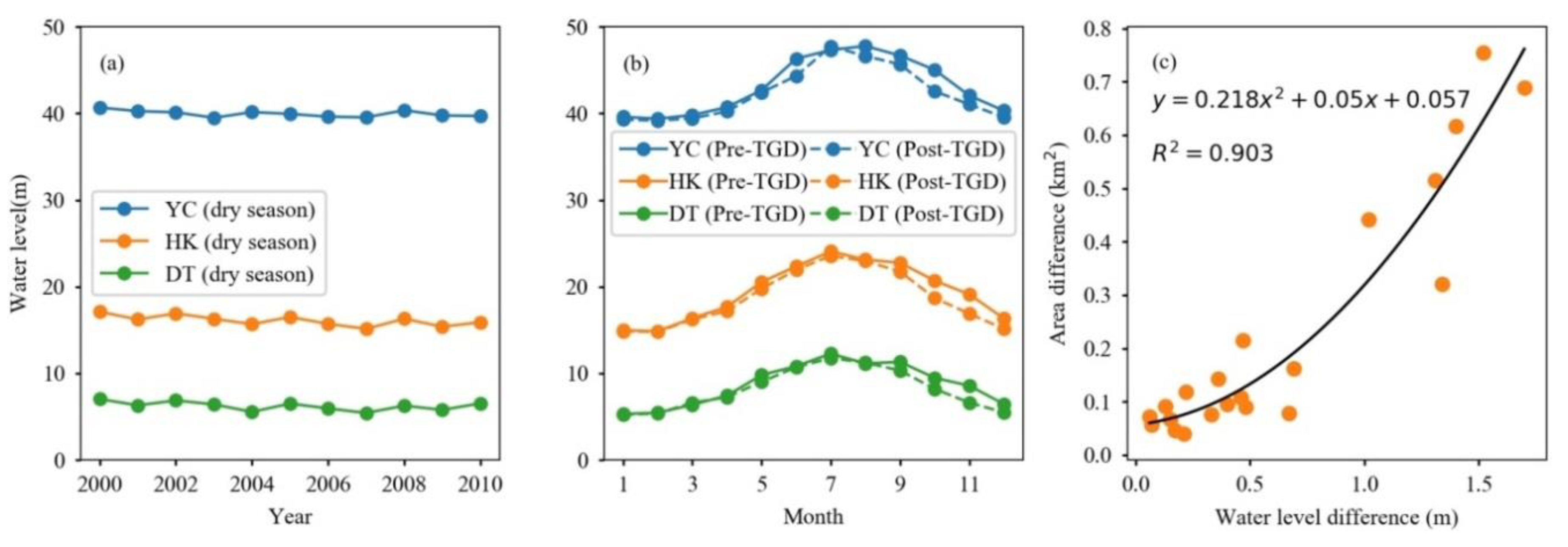
Not all Landsat images covering the study area were suitable for the analysis. A total of 553 images were carefully selected based on two criteria. First, the cloud cover should be less than 10% of the whole scene. Second, images should be acquired during the dry season (i.e., November to March) [24] for the following reasons. The presence of MCBs is largely affected by the water level at the imaging time [45]. Therefore, the water levels around the same MCBs should be identical for different imaging times, which is important for analyzing the temporal dynamics of MCBs. However, such an ideal requirement is unrealistic for the Landsat images acquired at a frequency of 16 days, and the practical way to proceed is to keep the water levels within a relatively small range rather than identical (Figure 2a). Moreover, the water level variation in the dry season is much smaller than that in the flood season (Figure 2b), which can minimize the uncertainty of the extracted MCB caused by water level fluctuation [46]. Generally, a 0.5 m change of water level could cause about 0.1 km2 area change of MCBs (Figure 2c).
2.2.2. High Spatial Resolution (HSR) Images
Using Google Earth, some HSR images were carefully selected as source data to obtain validation MCBs, which were then used to assess the accuracy of MCB extracted from the Landsat images. Since the presence and extent of MCB are highly dependent on the water level that varies over time, the acquisition dates of one Landsat image and the corresponding validation HSR image should be the same. However, this ideal criterion cannot always be met in practice. Therefore, this research used a more reasonable criterion: the difference of acquisition dates between HSR images and corresponding Landsat images is limited to 7 days. Finally, 19 HRS images were selected and downloaded from Google Earth (Table 1).
2.2.3. Gauged Datasets
River and suspended sediment discharges were collected at three key gauging stations (YC, HK, and DT) from the annually released Yangtze River Sediment Bulletin (http://www.cjw.gov.cn/zwzc/bmgb/). These data were yearly aggregated from daily measurements.
2.3. Producing MCBs
2.3.1. Extracting MCBs with Landsat Images
MCB is a land area surrounded by channel water. Therefore, the key to extracting MCB is to identify “holes” in channel water maps that can be produced from Landsat images. The procedure consists of five main steps as illustrated in Figure 3 and detailed below.
• Step 1: Clipping image
For each Landsat scene, the Yangtze River channel only occupies a small portion of the image, thus, it is necessary to clip out the small portion containing the Yangtze River channel from the entire Landsat scene to improve computing efficiency. The clipper is a 1-km buffered Yangtze River channel polygon which was manually delineated from Landsat 8 images (Figure 1).
• Step 2: Calculating water index
Landsat water indices have widely been used for mapping surface water bodies [47], for example, the normalized difference water index [48], the modified normalized difference water index (MNDWI) [49], and the automated water extraction index for images with and without considering shadows [50]. Previous studies have suggested that the MNDWI performs well in various conditions when compared to other water indices [50,51,52,53]. This study, therefore, adopted MNDWI. Equation (1) was applied to all the clipped satellite images to generate MNDWI images using a Python script with the ArcGIS software environment (version 10.3.0.4322, ESRI, Redlands, CA, USA) [54].
where ρgreen and ρswir1 are surface reflectance in the green band and the short-wave infrared band (i.e., band 5 for Landsat-4/5/7 and band 6 for Landsat 8), respectively.
• Step 3: Determining the optimal threshold
To classify channel water from the land area, an optimal threshold is needed to segment the MNDWI images. However, the optimal threshold often varies with space and time [52]. Since there are hundreds of MNDWI images, it is crucial to automatically determine the optimal threshold of each MNDWI image independently. The modified histogram bimodal method (MHBM) developed by Zhang et al. [53] was applied to determine the optimal threshold of each image. 548 out of 553 MNDWI images featured distinct bimodal histogram patterns which were very suitable for the application of MHBM. For the other five MNDWI images with non-bimodal histograms, the MCBs were extracted manually.
• Step 4: Classifying water and non-water areas
For an MNDWI image, pixels with values larger than the determined threshold were classified as water areas the others were classified as non-water areas.
• Step 5: Extracting MCBs
First, the raster format water body area were converted into vector shapefile polygons with smoothed edges. Next, the holes in the vector water map were converted to polygons that were considered as candidate MCBs. Geographically, all the holes contained in the channel water are MCBs. For the Yangtze River, however, some of the holes can also be large ships because this river is one of the busiest inland waterways in the world [55]. Such detected ships are often less than 0.02 km2, as confirmed by carefully inspecting the high spatial resolution images provided by Google Earth. Finally, the “true” MCBs were selected from the candidate MCBs with an area larger than 0.02 km2. All these processes were done by specific Python scripts in the ArcGIS environment (version 10.3.0.4322, ESRI, Redlands, CA, USA) [54].
2.3.2. Calculating MCBs’ Attributions
(1) Unique Coding
Each MCB generated from a Landsat scene was initially assigned a unique identification code. The code consists of three parts: the scene’s path and row numbers, the scene’s acquisition date, and the inherent geometry identification number of the MCB. For example, code “12103920100114005” means the corresponding MCB is identified as “005” in the scene which was obtained at path “121” and row “039” on date 14 January 2010. Therefore, each MCB had its own unique code, which could complicate the dynamic analysis of the MCB in the programming process. To avoid this inconvenience, the MCBs located at the same place but generated from different Landsat scenes with different acquisition dates should share the same code. In this study, the code that contains the earliest acquisition date was assigned to all the MCBs at the same location. The unique codes of all MCBs were listed in the supplementary Table S1.
(2) Area and shape index
Our analysis focused on area and shape attributes. Since MCBs often in transverse or lobate shapes [9], the length-width ratio (LWR, Equation (2)) may serve as an appropriate metric to indicate an MCB’s shape and its dynamics caused by deposition or erosion:
where L and W represent the length and width of the convex rectangle of an MCB, respectively. Both MCB’s area and convex rectangle were generated with the ArcGIS environment (version 10.3.0.4322, ESRI, Redlands, CA, USA) [54]. The area and LWR values of all MCBs were listed in the supplementary Table S1.
2.4. Processing Validation Data
The validation MCBs that occurred in the HSR images (Table 1) were manually delineated using ArcMap. The same MCBs but derived from Landsat images (Table 1) for accuracy assessment were also selected. In total, 49 pairs of MCBs (validation MCBs vs. assessment MCBs) were matched (see supplementary .kml files). Both their area and LWR values were calculated and were used for further accuracy assessment analysis.
2.5. Analysis Methods
Many geographical and environmental temporally dynamic phenomena experience structural breaks which could result from some sudden events, such as disasters or human intervention. Previous case studies have reported that the temporal dynamics of some MCBs might have been affected by the closure of TGD [12,28]. In our study, these temporal structural breaks were tested systematically. The Chow test [56] used by many other researchers [57,58] was applied to test TGD induced structural break. For a time series of MCBs data, the Chow test examined the null hypothesis: H0 (there is no structural change) vs. the alternative hypothesis H1 (there is a structural change). The test was conducted by running three separate regressions and an F-test: (1) a linear regression with the entire time series data; (2) two separate linear regressions with data before (Pre-TGD) and after TGD closure in 2003 (Post-TGD); and (3) an F-test to determine whether a single linear regression is more efficient than two separate regressions. If this F-test was significant (p-value < 0.05), the null hypothesis (H0) was rejected in favor of the alternative hypothesis (H1) was accepted. This process was applied to each individual MCB and grouped MCBs (as detailed in Section 3.2.2) in the R software environment [59].
3. Results
3.1. Understanding of the Extracted MCBs
3.1.1. Accuracy of Extracted MCBs Data
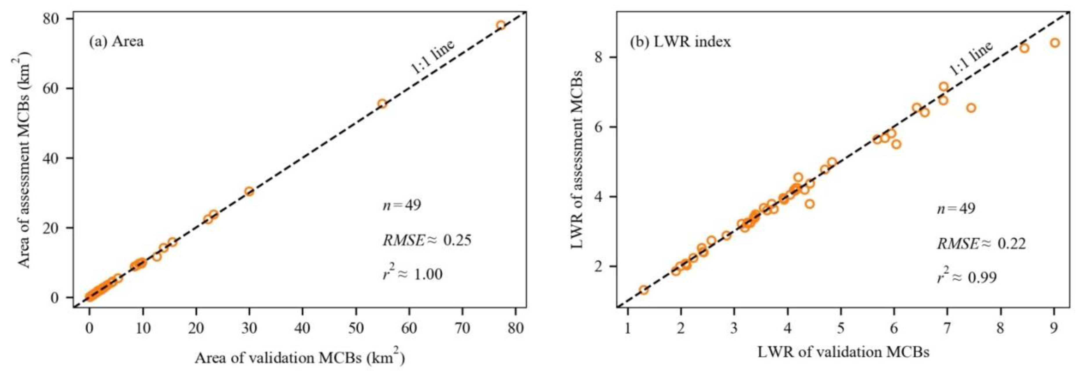
Accuracy of the MCBs extracted from Landsat images was assessed using the validation MCBs generated from HSR images. These validation MCBs were distributed along the entire study area (Table 1) and represent a wide range of MCB characteristics both in area (size) and shape (LWR) (Figure 4). For both area and shape, the Landsat derived MCBs are consistent with the validation MCBs. The Root Mean Square Error (RMSE) values for area and LRW were 0.25 km2 and 0.22, respectively. These results show that the accuracy of the procedures for extracting MCBs with Landsat images is acceptable and that the extracted MCBs are reliable for performing area and LWR dynamic analysis.
3.1.2. General Overview of MCBs
This study provides the first opportunity for examining the general pattern of MCBs downstream of TGD. The individual MCB area varies from 0.08 km2 to 223 km2 (Figure 5). Moreover, the area histogram illustrates a strong right-skewed distribution as shown in Figure 5a-1,a-2. Specifically, half of the MCBs are less than 2 km2, 25% of MCBs are within an area range from 2 km2 to 7 km2; 20% of MCBs within an area range from 7 km2 to 33 km2; and only 5% of MCBs are larger than 33 km2.
MCBs area is a comprehensive indicator of both geographical processes (e.g., geomorphology evolution stage, vegetation status, and stability) and anthropological processes (e.g., land use type, development history, and sand mining) [8,15]. Thus, the observed large variations in area between MCBs indicate that the dynamic analysis of MCBs should fully consider the potential influences caused by the effects of size or scale. It is necessary to group MCBs into different size types based on specific area criteria. To the best of our knowledge, however, there are no such criteria that can be referenced. Most of the previous studies focused on large MCBs which have relatively little area variation [12,30]. In this study, considering both the area histogram distribution (Figure 5a-1,a-2) and sample size requirements for further statistical analysis, MCBs were grouped into four size types, namely T1, T2, T3, and T4 (Table 2).
3.2. Spatiotemporal Dynamics of MCBs
3.2.1. Longitudinal Distribution
The longitudinal distribution of MCBs is illustrated in Figure 5. The distribution pattern is uneven (Figure 5c). In detail, distinct distribution patterns of MCBs were observed in middle reach (TGD-HK) and lower reach (HK-EST). In the middle reach, there are 42 MCBs (30% of the total number) scattered along the channel with an average interval of 15 km from 1985 to 2018. The sum of annual averaged MCBs area in the middle reach was 119 km2, accounting for 9% of the total MCBs area in the entire Yangtze River downstream of TGD (Figure 5b). By contrast, there were 98 MCBs (70% of total MCBs number) along the lower reach distributed with an average interval of 10 km, relatively denser than in the middle reach. The sum of annual averaged MCB area in lower reach was 1172 km2, accounting for 91% of the total MCBs area. These distinct longitudinal distribution patterns highlight the importance of the lower reach in the analysis of MCBs from both quality and quantity perspectives.
To be more specific, the MCBs extracted in 2016 were taken as an example to illustrate the longitudinal distribution patterns of MCBs (Figure 6). It is noteworthy that the T1 MCBs (i.e., small-size) scattered along the entire reach without obvious concentration. Most of the T2 and T3 MCBs (i.e., middle and large sizes) occurred in the lower reach. All of the T4 MCBs (i.e., extra-large size) were distributed in the lowest reach, i.e., JJ-EST (Figure 6a). In other words, MCBs with large area tended to be located farther downstream from TGD, especially in the reach JJ-EST.
3.2.2. Temporal Dynamics of MCBs
The temporal dynamics of MCBs in terms of number, area, and LWR indices are described below. For each index, this study performed analyses with and without consideration of MCB type. For each temporal trend analysis, whether the closure of TGD can be considered as a structural change during the whole period was also tested. If it did, the pre-TGD, post-TGD, and the overall regressions were applied; otherwise, only the overall regression was applied.
(1) Number
There was no statistically significant change in MCB number during the whole study period as shown in Figure 7a (a = −0.08, p-value > 0.05). However, TGD closure year (in 2003) was detected as a structural change and different trends were observed between the pre-TGD and post-TGD periods. In the pre-TGD period, MCB number showed an increasing trend (a = 0.4 and p-value < 0.01). Such a trend was reversed in the post-TGD period in which a significant decreasing trend was detected (a = −0.5, p-value < 0.01). To further understand these changes, trends of the four MCB types were checked as illustrated in Figure 7b–e. The number of T1 MCBs showed very similar trends as the total MCBs and the number in other three MCB types remained stable during the study period, suggesting that the phenomenon of MCB’s “disappearance” or “appearance” existed in the study periods and only happened for the small size MCBs (T1). It should be noted that the so-called “disappearance” or “appearance” does not mean an MCB completely disappeared or appeared. This is because only the candidate MCBs with an area larger than 0.02 km2 were detected (as explained in Section 2.3.1) and applied in our analysis. Therefore, in some cases, the “disappearance” of one MCB may be caused by flow erosion which reduced its area less than our detection criterion (0.02 km2).
Since the number change only occurred on T1 MCBs, where and when did these events happen is another question. As shown in Figure 8, the appearance of new MCBs mainly happened in the pre-TGD period. The locations of those events were concentrated in the JJ-EST reach. The MCB disappearance started in 1996 and mainly occurred in the JJ-EST reach as well. It is unexpected that the immediate downstream reach of TGD (i.e., TGD-HK) only experienced two events of MCB disappearance after the closure of TGD in 2003.
(2) Area
Overall, the area of all MCBs experienced an increasing trend with a slope of 2.77 km2/yr (p-value < 0.01, Figure 9a). The area of the four MCB types exhibited increasing trends (the trend for T3 is not statistically significant). The slopes of T1, T2, and T4 increased accordingly (Figure 9), from 0.53 km2/yr (p-value < 0.01) to 0.61 km2/yr (p-value < 0.01) to 1.29 km2/yr (p-value < 0.01). It is also noteworthy that the Coefficient of Variation (CV) values show a decreasing pattern from T1 to T4. The combination of these observations shows that larger MCBs tend to have higher rates of area increase (i.e., more sediment deposition) but with less area variation (i.e., more stability).
As for TGD effects on MCB area dynamics, structural changes were detected for T1 and T2 MCBs, but not for the T3 and T4 MCBs (Figure 9). For T1 and T2 MCBs, their area showed increasing trends in the pre-TGD period but showed slightly decreasing trends post-TGD. This result suggests that the closure of TGD might have a significant impact on area dynamics of small (T1) and middle (T2) size MCBs. In other words, smaller size MCBs are more likely to be influenced by the dam operation and experience more sediment erosion, whereas larger size MCBs probably have more resistance to the impact of dam operation.
(3) LWR shape index
Different types of MCBs had distinct basic shape characteristics as shown in Figure 10. Generally, the larger size MCBs have smaller LWR values (i.e., μ values in Figure 10), namely, 4.97 (T1) > 4.12 (T2) > 3.16 (T3) > 2.24(T4). According to the definition of LWR, this observation illustrates that the relatively small size MCBs (e.g., T1 and T2) tended to elongate, whereas relatively large size MCBs (e.g., T3 and T4) tended to appear more rounded in shape.
As for the overall temporal dynamics, it is noted that the LWR of the total MCBs showed a significant decreasing trend in the whole study period (a = −0.02, p-value < 0.01, Figure 10a), indicating that the shape of MCBs tended to change from elongate to relatively round. As for the different types of MCBs, their shape temporal dynamics illustrated distinct trends. T1 and T2 MCBs showed significant decreasing trends, while T3 and T4 MCBs showed a significant increasing trend in the whole period (Figure 10b–e). These results show that the T1 and T2 MCBs were gradually becoming relatively round whereas the T3 and T4 MCBs tended to become more elongate from 1989 to 2017. Apart from their change direction, their change rates also showed an interesting pattern: the larger size MCBs, the slower change rate of LWR dynamics, i.e., 0.03 /yr (T1) > 0.02 /yr (T2) > 0.01 /yr (T3) > 0.001 (T4). This pattern indicates that the shapes of T3 and T4 MCBs were more stable than those of T1 and T2 MCBs.
Structural changes were also detected in the LWR dynamics of T1, T2, and T3 MCBs at TGD closure year. For T1 MCBs (Figure 10b), they experienced an insignificant trend change in the pre-TGD period and a significantly decreasing trend in the post-TGD period. Both T2 and T3 MCBs showed a significant increasing trend in the post-TGD period (Figure 10c,d).
4. Discussion
4.1. Scale Effects on the Temporal Dynamics
The temporal dynamics of MCBs indicate that different MCB types had distinct trend characteristics. More specifically, the large MCBs seem to have more stability than the relatively small ones in terms of variations in both area and LWR. In other words, the size of MCBs may influence their temporal dynamics, which suggests the presence of scale effects. Figure 11 illustrates the scale effects of MCBs on the temporal stabilities of area and LWR in the overall, pre-TGD, and post-TGD periods, respectively. As for the overall period, the CV of area and LWR were both decreasing (becoming less variable and more stable) as the size or scale of the MCBs increased. Such a pattern also applies to the pre-TGD, and post-TGD periods. These results imply that the larger the size of MCB, the greater relative stability in area and shape variations, whereas the smaller size of the MCBs, the less stable in terms of area and shape variations. In previous studies, only one specific scale MCBs were focused (such as large-size MCBs), and the temporal dynamic patterns of other sizes of MCBs were not addressed [23,30].
Three reasons could explain the observed scale effect. The first is the growth of vegetation. Compared to small MCBs, large MCBs are more likely to be covered by vegetation [60,61]. In turn, the vegetation would provide more resistance to external forces such as sediment erosion [15,62]. The second is the strength of human interventions. Large size MCBs are more likely to have been occupied and modified by human beings and thus received more protection that can, in turn, enhance their stability. For example, people would harden MCB banks to prevent them from being eroded, especially on agriculturalized or industrialized MCBs in the lower reach [63]. The third is the effects of flooding. Generally, the small size MCBs have short evolution histories with lower height compared to the large size MCBs. Therefore, they are more likely to be inundated in a flooding event and to experience large variations in sediment erosion or deposition [64]. In contrast, large size MCBs would experience relatively fewer impacts by such flooding events.
4.2. Potential Effects of TGD Operation
It has been widely acknowledged that MCBs can be heavily influenced by flow and sediment regimes [31,62]. Downstream of TGD, marked changes of flow and sediment regimes between the pre- and post-TGD periods have been observed [39,65]. Although many previous studies focused on different periods, some common themes can be identified. First, there is no significant change in the annual water discharge between pre-TGD and post-TGD periods in the last three decades [24] (Figure 12a). However, the peak river discharge during the flood season was reduced due to the operation of TGD (Figure 12c). Second, the amount of sediment carried by the river started to decrease in the 1990s, but it dropped dramatically after TGD closure in 2003 (Figure 12b) [66]. Third, the sediment carrying capacity decreased in the lower reach [12,67]. The direct result of these changes is that the water immediately downstream of TGD is in a sediment-hungry condition, which would carry away some sediment in the riverbed or in the submerged parts of MCBs [68].
The operation of TGD could have impacted the temporal dynamics of MCBs in the downstream reach. A further question that needs to be discussed is whether these influences vary spatially as a function of the distance of MCBs to TGD. The frequency of structural changes (FSC) is proposed here as an indicator for analyzing this question. The FSC is identified as the frequency of temporal structural changed MCBs among every 10-MCBs bin. The temporal structural changes were tested for both area and shape metrics between pre-TGD and post-TGD periods (see Section 2.5). For a bin, the 10 MCBs are counted in ascending order by their distances to TGD. Therefore, the higher the FSC, the more likely the structural changes were caused by TGD operation (Figure 13a).
For area temporal dynamics, the FSC gradually decreased from 0.7 to 0.2 in TGD-JJ reach, and then slowly increased from 0.2 to 0.8 in the JJ-NJ reach (Figure 13a). Similarly, the FSC of LWR gradually decreased from 0.7 to 0.3 in TGD-HK reach, and then slowly increased from 0.3 to 0.8 in the HK-DT reach. The decreasing patterns of FSC indicate that, to some extent, the effects of TGD operation decreased as the distance to TGD increased. The minimum effects of TGD occurred at HK and JJ for the LWR dynamics and area dynamics, respectively. This result is similar to observations made in previous studies that focused on the effects of TGD on the water regime and channel dynamics [46,69]. For example, [46] found that the operation of TGD reduced the water level in the river downstream, but the effects were most pronounced immediately downstream of the dam and generally diminished in a longitudinal direction from TGD to the estuary. As for the channel dynamics, Yuan et al., [69] reported that channel scour was found in the post-TGD period and was strongest immediately downstream of the dam and then decreased longitudinally. In contrast, this study noted an unexpected increasing trend of FSC in the HK-DT and JJ-NJ reaches for the LWR and area dynamics, respectively. Do these results imply the TGD effects increased in these lower reaches after the effects had been considered minor as discussed just above? It may be unreasonable to make such a judgment and thus more evidence is needed to explain the increasing trend we observed in this study. In fact, apart from the aforementioned hydrological factors, some human activities, such as sand mining, may also play an important role in changing the MCB area and LWR dynamics [16], especially for the middle- and small-size MCBs in the lower reach like JJ-DT. Before 2003, sand mining activity was banned. However, after carrying out the Regulation of Sand Mining Management in the Yangtze River in June 2003, the amount of annual sand mining increased dramatically (Figure 13b). Those sand mining activities that were reported mainly in the lower reach, particularly in the JJ-EST reach [70]. Since the large-scale sand mining activities often happened near MCBs [71], it could cause a structural change of MCBs dynamics after 2003. Therefore, the causes for MCBs’ dynamics in the lower reach (JJ-EST) is more complicated than that in the reach immediately downstream of TGD (TGD-HK) and more supporting data and quantitative analysis are needed for the further evaluation of TGD effects on the lower reach.
In addition to the longitudinal extent of TGD effects, this study was also interested in how the TGD effects were expressed. Figure 14 indicates that the majority of MCBs experiencing a structural change habited an opposite trend in the post-TGD period compared to the pre-TGD period. Specifically, 72 out of 140 MCBs showed PR structural change (positive in pre-TGD and negative in post-TGD) in area temporal dynamics and 79 out of 140 MCBs experienced NR structural change (negative in pre-TGD and positive in post-TGD) in LWR temporal dynamics. This observation suggests that the operation of TGD could be the driving force that caused over half of MCBs to experience erosion (decreasing area) and became elongate (increasing LWR) in the post-TGD period. Thus, the operation of TGD could have significant impacts on the dynamics of MCBs in the Yangtze River downstream.
4.3. Limitation and Future Research
Similar to many studies, there are several limitations and open issues associated with our current research. The area and shape of image-extracted MCBs are influenced by the water level variation due to the different image acquisition dates as demonstrated in Figure 2c. Although this unwelcome factor has been carefully considered with our best effort during the data preparation, some uncertainties could still be introduced to the temporal dynamic analyses of area and LWR. In the future studies, two further improvements can be made to minimize the impacts of such uncertainties. First, the temporal dynamics analysis should focus on a group of MCBs rather than individual MCBs and the conclusions should be made from a statistical point of view [72]. Second, future research can use new high-spatiotemporal-resolution RS images, such as PlanetScope [73], which can enable greater consistency of water levels on different acquisition dates. The second improvement is highly recommended in the future MCBs monitoring works as these data can be obtained more economically in the near future.
Due to the relatively coarse spatial resolution of Landsat images (30 m) and the complex conditions of the Yangtze River, this study used 0.02 km2 as an area threshold to determine the MCBs, i.e., only the image-extracted patches larger than 0.02 km2 were considered as MCBs. As a result, some MCBs less than 0.02 km2 were excluded in the analysis. In the future study, however, these tiny MCBs should also be manually checked by experts or by using high spatial resolution images to pick them out of the real non-MCBs objects, such as large ships and some man-made features.
In a real riverine system, MCBs not only experience area and shape dynamics in two-dimensional (2D) space but also experience volume and location dynamics in three-dimensional (3D) space [6,16]. To fully understand MCB dynamics and the effects of TGD, more work needs to be conducted in monitoring MCB location migrating and sand volume change. Such work will increase our understanding of sediment transportation and water management in the Yangtze River [39].
5. Conclusions
This study presents a systematic analysis of MCBs in the entire Yangtze River downstream of TGD in the last three decades. It gives us the first opportunity to comprehensively understand the longitudinal and temporal dynamics of MCBs during pre- and post-TGD periods. Most of the MCBs in terms of number (98 out of 140) and total area (1172 km2 out of 1291 km2) were scattered in the lower reach (HK-EST) with an average interval of 10 km along the channel. The temporal dynamics patterns were examined using annual MCB data using a statistical classification system. This classification system grouped the extracted 140 MCBs into four general size-types based on their area distribution. The four size-types are T1 small (area < 2km2), T2 middle (area between 2 km2 and 7 km2), T3 large (area between 7 km2 and 33 km2), and T4 extra-large (area > 33 km2) MCBs. For each type, the MCB temporal dynamics in total number, area, and shape index (i.e., LWR) were comparatively analyzed during the before and after TGD operation periods.
Overall, the number of MCBs increased before TGD operation and then declined significantly after the TGD operation. As for the different MCB types, only the T1 MCBs experienced such a change in number and most of this change happened in the lower reach. Although the area of all types of MCB showed an overall increasing trend, large size MCBs tended to experience larger change rate and less variation than that of the small size MCBs. Large size MCBs seemed to experience fewer impacts of TGD on their area dynamics whereas the small size MCBs likely were more influenced by the TGD operation. As for the shape dynamics, small size and middle size MCBs tended to become relatively more rounded in shape whereas the large and extra-large size MCB tended to become more elongate. Similarly, the shape dynamics of the large MCBs were more stable than those of small MCBs. This study implies that the scale (size) effects of MCBs on their temporal dynamics need to be paid more attention in future MCB analysis or in the practical management of MCBs such as channel dredging.
The operation of TGD could have significant effects on MCB dynamics. This study showed that the strength of such effects decreased as the distance to TGD increased, and minimized at HK (for LWR dynamics) or JJ (area dynamics). In contrast, the driving forces of the MCB dynamics in the lowest JJ-EST reach are more complex as more external influences such as sand mining activities are observed in the area and additional analyses are needed in the future.
Supplementary Materials
The following are available online at https://www.mdpi.com/2072-4292/12/3/409/s1, Table S1, Table S2, kml files.
Author Contributions
Conceptualization, Z.W. and S.W.; methodology, Z.W. and C.Z.; formal analysis, Z.W.; investigation, Z.W.; resources, Z.W. and G.S.; data curation, Z.W.; writing—original draft preparation, Z.W.; writing—review and editing, H.Y., C.Z., and G.S.; visualization, Z.W.; supervision, H.Y. and S.W.; funding acquisition, Z.W. and H.Y. All authors have read and agree to the published version of the manuscript.
Funding
This research was jointly funded by the National Natural Science Foundation of China (No: 41501096 and 51779241), Open Fund of State Laboratory of Information Engineering in Surveying, Mapping and Remote Sensing, Wuhan University (No: 18R07), and the Open Fund of State Key Laboratory of Lake Science and Environment, Chinese Academy of Sciences (No: 2018SKL006).
Acknowledgments
The authors would like to thank the reviewers for valuable input that increased the quality of this paper.
Conflicts of Interest
The authors declare no conflict of interest.
References
- Freyer, J.B.; Jefferson, A.J. An exception to island loss in the engineered upper Mississippi River: History of land growth in Pool 6 and implications for restoration. Anthropocene 2013, 2, 65–75. [Google Scholar] [CrossRef]
- Hecht, J.S.; Lacombe, G.; Arias, M.E.; Dang, T.D.; Piman, T. Hydropower dams of the Mekong River basin: a review of their hydrological impacts. J. Hydrol. 2019, 568, 285–300. [Google Scholar] [CrossRef]
- Yang, H.; Flower, R.J. Potentially massive greenhouse-gas sources in proposed tropical dams. Front. Ecol. Environ. 2012, 10, 234–235. [Google Scholar] [CrossRef]
- Liermann, C.R.; Nilsson, C.; Robertson, J.; Ng, R.Y. Implications of dam obstruction for global freshwater fish diversity. Bioscience 2012, 62, 539–548. [Google Scholar] [CrossRef]
- Schmutz, S.; Moog, O. Dams: Ecological impacts and management. In Riverine Ecosystem Management; Springer: Cham, Switzerland, 2018; pp. 111–127. [Google Scholar]
- Adami, L.; Bertoldi, W.; Zolezzi, G. Multidecadal dynamics of alternate bars in the Alpine Rhine River. Water Resour. Res. 2016, 52, 8938–8955. [Google Scholar] [CrossRef]
- Osterkamp, W.R. Processes of fluvial island formation, with examples from Plum Creek, Colorado and Snake River, Idaho. Wetlands 1998, 18, 530–545. [Google Scholar] [CrossRef]
- Ashworth, P.J. Mid-channel bar growth and its relationship to local flow strength and direction. Earth Surf. Process. Landf. 1996, 21, 103–123. [Google Scholar] [CrossRef]
- Hooke, J.M. The significance of mid-channel bars in an active meandering river. Sedimentology 1986, 33, 839–850. [Google Scholar] [CrossRef]
- Wintenberger, C.L.; Rodrigues, S.; Claude, N.; Juge, P.; Breheret, J.G.; Villar, M. Dynamics of nonmigrating mid-channel bar and superimposed dunes in a sandy-gravelly river (Loire River, France). Geomorphology 2015, 248, 185–204. [Google Scholar] [CrossRef]
- Xu, J.X. Evolution of mid-channel bars in a braided river and complex response to reservoir construction: An example from the middle Hanjiang River, China. Earth Surf. Process. Landf. 1997, 22, 953–965. [Google Scholar]
- Lou, Y.Y.; Mei, X.F.; Dai, Z.J.; Wang, J.; Wei, W. Evolution of the mid-channel bars in the middle and lower reaches of the Changjiang (Yangtze) River from 1989 to 2014 based on the Landsat satellite images: Impact of the Three Gorges Dam. Environ. Earth Sci. 2018, 77, 394. [Google Scholar] [CrossRef]
- Tabacchi, E.; Steiger, J.; Corenblit, D.; Monaghan, M.T.; Planty-Tabacchi, A.-M. Implications of biological and physical diversity for resilience and resistance patterns within Highly Dynamic River Systems. Aquat. Sci. 2009, 71, 279. [Google Scholar] [CrossRef] [Green Version]
- Tonkin, J.D.; Merritt, D.M.; Olden, J.D.; Reynolds, L.V.; Lytle, D.A. Flow regime alteration degrades ecological networks in riparian ecosystems. Nat. Ecol. Evol. 2018, 2, 86–93. [Google Scholar] [CrossRef] [PubMed]
- Hooke, J.M.; Yorke, L. Channel bar dynamics on multi-decadal timescales in an active meandering river. Earth Surf. Process. Landf. 2011, 36, 1910–1928. [Google Scholar] [CrossRef]
- Wang, B. Assessing Morphodynamics of the Lower Mississippi River from 1985 to 2015 with Remote Sensing and GIS Techniques. Ph.D. Thesis, Louisiana State University, Baton Rouge, LA, USA, 2017. [Google Scholar]
- Han, J.Q.; Zhang, W.; Fan, Y.Y.; Yu, M.Q. Interacting effects of multiple factors on the morphological evolution of the meandering reaches downstream the Three Gorges Dam. J. Geogr. Sci. 2017, 27, 1268–1278. [Google Scholar] [CrossRef] [Green Version]
- Nelson, N.C.; Erwin, S.O.; Schmidt, J.C. Spatial and temporal patterns in channel change on the Snake River downstream from Jackson Lake dam, Wyoming. Geomorphology 2013, 200, 132–142. [Google Scholar] [CrossRef]
- Petts, G.E. Complex response of river channel morphology subsequent to reservoir construction. Prog. Phys. Geogr. 1979, 3, 329–362. [Google Scholar] [CrossRef]
- Erskine, W.D. Downstream geomorphic impacts of large dams: The case of Glenbawn Dam, NSW. Appl. Geogr. 1985, 5, 195–210. [Google Scholar] [CrossRef]
- Graf, W.L. Downstream hydrologic and geomorphic effects of large dams on American rivers. Geomorphology 2006, 79, 336–360. [Google Scholar] [CrossRef]
- Provansal, M.; Dufour, S.; Sabatier, F.; Anthony, E.J.; Raccasi, G.; Robresco, S. The geomorphic evolution and sediment balance of the lower Rhône River (southern France) over the last 130 years: Hydropower dams versus other control factors. Geomorphology 2014, 219, 27–41. [Google Scholar] [CrossRef]
- Wang, J.; Dai, Z.J.; Mei, X.F.; Lou, Y.Y.; Wei, W.; Ge, Z.P. Immediately downstream effects of Three Gorges Dam on channel sandbars morphodynamics between Yichang-Chenglingji Reach of the Changjiang River, China. J. Geogr. Sci. 2018, 28, 629–646. [Google Scholar] [CrossRef] [Green Version]
- Dai, Z.; Liu, J.T. Impacts of large dams on downstream fluvial sedimentation: An example of the Three Gorges Dam (TGD) on the Changjiang (Yangtze River). J. Hydrol. 2013, 480, 10–18. [Google Scholar] [CrossRef]
- Xu, J.; Yin, R.; Li, Z.; Liu, C. China’s ecological rehabilitation: Unprecedented efforts, dramatic impacts, and requisite policies. Ecol. Econ. 2006, 57, 595–607. [Google Scholar] [CrossRef]
- Yang, C.S.; Ouchi, K. Analysis of bar morphology using multi-temporal and multi-sensor satellite images: Example from the Han Estuary, Korea. Mar. Geol. 2012, 311, 17–31. [Google Scholar] [CrossRef]
- Zheng, S.W.; Xu, Y.J.; Cheng, H.Q.; Wang, B.; Xu, W.; Wu, S.H. Riverbed erosion of the final 565 kilometers of the Yangtze River (Changjiang) following construction of the Three Gorges Dam. Sci. Rep.-UK 2018, 8, 11917. [Google Scholar] [CrossRef]
- Gao, B.; Yang, D.; Yang, H. Impact of the Three Gorges Dam on flow regime in the middle and lower Yangtze River. Quatern. Int. 2013, 304, 43–50. [Google Scholar] [CrossRef]
- Baki, A.B.M.; Gan, T.Y. Riverbank migration and island dynamics of the braided Jamuna River of the Ganges-Brahmaputra basin using multi-temporal Landsat images. Quatern. Int. 2012, 263, 148–161. [Google Scholar] [CrossRef]
- Gao, C.; Chen, S.; Yu, J. River islands’ change and impacting factors in the lower reaches of the Yangtze River based on remote sensing. Quatern. Int. 2013, 304, 13–21. [Google Scholar] [CrossRef]
- Raška, P.; Dolejš, M.; Hofmanová, M. Effects of damming on long-term development of fluvial islands, Elbe River (N Czechia). River research and applications. 2017, 33, 471–482. [Google Scholar] [CrossRef]
- Sanford, J.P. Dam Regulations Effects on Sand Bar Migration on the Missouri River: Southeastern South Dakota. Bachelor’s Thesis, University of Montana, Missoula, MT, USA, 2007. [Google Scholar]
- Kiss, T.; Balogh, M. Characteristics of point-bar development under the influence of a dam: Case study on the Dráva River at Sigetec, Croatia. J. Environ. Geogr. 2015, 8, 23–30. [Google Scholar] [CrossRef] [Green Version]
- Piégay, H.; Grant, G.; Nakamura, F.; Trustrum, N. Braided river management: from assessment of river behaviour to improved sustainable development. In Braided Rivers: Process, Deposits, Ecology and Management; Smith, G.H.S., Best, J.L., Bristow, C.S., Petts, G.E., Eds.; Blackwell Publishing: Malden, MA. USA, 2006; pp. 257–275. [Google Scholar]
- Lyu, Y.; Zheng, S.; Tan, G.; Shu, C.; Han, Q. Morphodynamic adjustments in the Yichang–Chenglingji Reach of the Middle Yangtze River since the operation of the Three Gorges Project. CATENA 2019, 172, 274–284. [Google Scholar] [CrossRef]
- Yang, S.L.; Milliman, J.D.; Li, P.; Xu, K. 50,000 dams later: Erosion of the Yangtze River and its delta. Glob. Planet. Chang. 2011, 75, 14–20. [Google Scholar] [CrossRef]
- Wang, B.; Xu, Y.J. Decadal-Scale Riverbed Deformation and Sand Budget of the Last 500 km of the Mississippi River: Insights Into Natural and River Engineering Effects on a Large Alluvial River. J. Geophys. Res.-Earth Surf. 2018, 123, 874–890. [Google Scholar] [CrossRef]
- Han, X.; Chen, X.; Feng, L. Four decades of winter wetland changes in Poyang Lake based on Landsat observations between 1973 and 2013. Remote Sens. Environ. 2015, 156, 426–437. [Google Scholar] [CrossRef]
- Yang, S.L.; Milliman, J.D.; Xu, K.H.; Deng, B.; Zhang, X.Y.; Luo, X.X. Downstream sedimentary and geomorphic impacts of the Three Gorges Dam on the Yangtze River. Earth-Sci. Rev. 2014, 138, 469–486. [Google Scholar] [CrossRef]
- Liu, J.; Li, S.; Ouyang, Z.; Tam, C.; Chen, X. Ecological and socioeconomic effects of China’s policies for ecosystem services. Proc. Natl. Acad. Sci. USA 2008, 105, 9477–9482. [Google Scholar] [CrossRef] [PubMed] [Green Version]
- Masek, J.G.; Vermote, E.F.; Saleous, N.E.; Wolfe, R.; Hall, F.G.; Huemmrich, K.F.; Feng, G.; Kutler, J.; Teng-Kui, L. A Landsat surface reflectance dataset for North America, 1990-2000. IEEE Trans. Geosci. Remote. Sens. 2006, 3, 68–72. [Google Scholar] [CrossRef]
- Product Guide. Landsat 4-7 Surface Reflectance (LEDAPS) Product; Department of the Interior U.S. Geological Survey: Reston, VG, USA, 2018.
- Product Guide. Landsat 8 Surface Reflectance Code (LASRC) Product; Department of the Interior U.S. Geological Survey: Reston, VG, USA, 2018.
- Young, N.E.; Anderson, R.S.; Chignell, S.M.; Vorster, A.G.; Lawrence, R.; Evangelista, P.H. A survival guide to Landsat preprocessing. Ecology 2017, 98, 920–932. [Google Scholar] [CrossRef] [Green Version]
- Ham, D.G.; Church, M. Bed-material transport estimated from channel morphodynamics: Chilliwack River, British Columbia. Earth Surf. Process. Landforms. 2000, 25, 1123–1142. [Google Scholar] [CrossRef]
- Wang, J.; Sheng, Y.; Gleason, C.J.; Wada, Y. Downstream Yangtze River levels impacted by Three Gorges Dam. Environ. Res. Lett. 2013, 8, 044012. [Google Scholar] [CrossRef]
- Verpoorter, C.; Kutser, T.; Seekell, D.A.; Tranvik, L.J. A global inventory of lakes based on high-resolution satellite imagery. Geophys. Res. Lett. 2014, 41, 6396–6402. [Google Scholar] [CrossRef]
- McFeeters, S.K. The use of the Normalized Difference Water Index (NDWI) in the delineation of open water features. Int. J. Remote Sens. 1996, 17, 1425–1432. [Google Scholar] [CrossRef]
- Xu, H.Q. Modification of normalised difference water index (NDWI) to enhance open water features in remotely sensed imagery. Int. J. Remote Sens. 2006, 27, 3025–3033. [Google Scholar] [CrossRef]
- Feyisa, G.L.; Meilby, H.; Fensholt, R.; Proud, S.R. Automated water extraction index: A new technique for surface water mapping using Landsat imagery. Remote Sens. Environ. 2014, 140, 23–35. [Google Scholar] [CrossRef]
- Fisher, A.; Flood, N.; Danaher, T. Comparing Landsat water index methods for automated water classification in eastern Australia. Remote Sens. Environ. 2016, 175, 167–182. [Google Scholar] [CrossRef]
- Ji, L.; Zhang, L.; Wylie, B. Analysis of dynamic thresholds for the normalized difference water index. Photogramm. Eng. Remote Sensing 2009, 75, 1307–1317. [Google Scholar] [CrossRef]
- Zhang, F.F.; Li, J.S.; Zhang, B.; Shen, Q.; Ye, H.P.; Wang, S.L.; Lu, Z.Y. A simple automated dynamic threshold extraction method for the classification of large water bodies from landsat-8 OLI water index images. Int. J. Remote Sens. 2018, 39, 3429–3451. [Google Scholar] [CrossRef]
- ESRI. ArcGIS desktop: Release 10.3; Environmental Systems Research Institute: Redlands, CA, USA, 2014. [Google Scholar]
- Zhang, D.; Yan, X.; Yang, Z.; Wang, J. An accident data–based approach for congestion risk assessment of inland waterways: A Yangtze River case. P. I. Mech. Eng. O-J. Ris. 2014, 228, 176–188. [Google Scholar] [CrossRef]
- Chow, G.C. Tests of equality between sets of coefficients in two linear regressions. Econometrica 1960, 28, 591–605. [Google Scholar] [CrossRef]
- Lee, T.S. Change-point problems: bibliography and review. J. Stat. Theory Pract. 2010, 4, 643–662. [Google Scholar] [CrossRef]
- Lewis, L.Y.; Landry, C.E. River restoration and hedonic property value analyses: Guidance for effective benefit transfer. Water Resour. Econ. 2017, 17, 20–31. [Google Scholar] [CrossRef]
- R Core Team. R: A Language and Environment for Statistical Computing. 2013. Available online: https://repo.bppt.go.id/cran/web/packages/dplR/vignettes/intro-dplR.pdf (accessed on 26 January 2020).
- Asaeda, T.; Rashid, M.H. The impacts of sediment released from dams on downstream sediment bar vegetation. J. Hydrol. 2012, 430, 25–38. [Google Scholar] [CrossRef]
- Osterkamp, W.R.; Hupp, C.R. Fluvial processes and vegetation - Glimpses of the past, the present, and perhaps the future. Geomorphology 2010, 116, 274–285. [Google Scholar] [CrossRef]
- Gilvear, D.; Willby, N. Channel dynamics and geomorphic variability as controls on gravel bar vegetation; River Tummel, Scotland. River Res. Appl. 2006, 22, 457–474. [Google Scholar] [CrossRef]
- Gregory, K. The human role in changing river channels. Geomorphology 2006, 79, 172–191. [Google Scholar] [CrossRef]
- Wang, Z.; Li, H.; Cai, X. Remotely sensed analysis of channel bar morphodynamics in the middle Yangtze River in response to a major monsoon flood in 2002. Remote Sens. BASEL 2018, 10, 1165. [Google Scholar] [CrossRef] [Green Version]
- Mei, X.; Dai, Z.; Van Gelder, P.; Gao, J. Linking Three Gorges Dam and downstream hydrological regimes along the Yangtze River, China. Earth Space Sci. 2015, 2, 94–106. [Google Scholar] [CrossRef]
- Wang, Y.K.; Rhoads, B.L.; Wang, D.; Wu, J.C.; Zhang, X. Impacts of large dams on the complexity of suspended sediment dynamics in the Yangtze River. J. Hydrol. 2018, 558, 184–195. [Google Scholar] [CrossRef]
- Lai, X.; Yin, D.; Finlayson, B.L.; Wei, T.; Li, M.; Yuan, W.; Yang, S.; Dai, Z.; Gao, S.; Chen, Z. Will river erosion below the Three Gorges Dam stop in the middle Yangtze? J. Hydrol. 2017, 554, 24–31. [Google Scholar] [CrossRef]
- Yang, C.; Cai, X.B.; Wang, X.L.; Yan, R.R.; Zhang, T.; Zhang, Q.; Lu, X.R. Remotely Sensed Trajectory Analysis of Channel Migration in Lower Jingjiang Reach during the Period of 1983–2013. Remote Sens. 2015, 7, 16241–16256. [Google Scholar] [CrossRef] [Green Version]
- Yuan, W.H.; Yin, D.W.; Finlayson, B.; Chen, Z.Y. Assessing the potential for change in the middle Yangtze River channel following impoundment of the Three Gorges Dam. Geomorphology 2012, 147, 27–34. [Google Scholar] [CrossRef]
- Changjiang Water Resources Commission. Changjiang Sediment Bulletin; Changjiang Water Resources Commission: Wuhan, China, 2003–2017. Available online: http://www.cjw.gov.cn/zwzc/bmgb/ (accessed on 26 January 2020).
- Lai, X.J.; Jiang, J.H.; Yang, G.S.; Lu, X.X. Should the Three Gorges Dam be blamed for the extremely low water levels in the middle-lower Yangtze River? Hydrol. Process. 2014, 28, 150–160. [Google Scholar] [CrossRef]
- Dalvi, N.; Suciu, D. Answering queries from statistics and probabilistic views. In Proceedings of the 31st International Conference on Very Large Data Bases, Trondheim, Norway, 30 August–4 September 2005; pp. 805–816. [Google Scholar]
- Planet Team. Planet Application Program Interface: In Space for Life on Earth. San Francisco, CA, USA. Available online: https://www.planet.com (accessed on 26 January 2020).
Figure 1.
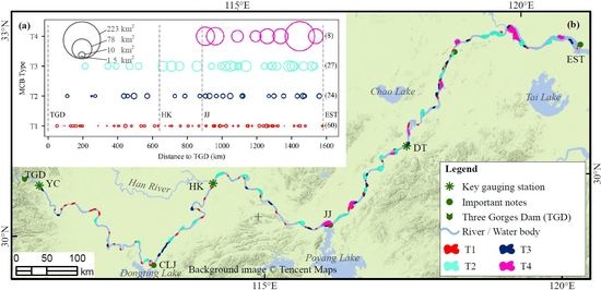
Geographic location of the study area (downstream of the Three Gorges Dam or TGD) and corresponding footprints of Landsat 4/5/7/8 images. Location names, TGD, YC, CLJ, HK, JJ, DT, NJ, and EST, are the acronym of Three Gorges Dam, Yichang, Chenglinji, Hankou, Jiujiang, Datong, Nanjing and estuary of the Yangtze River, respectively. The closed number following location name indicates the downward distance of that location from TGD. For example, “YC (43km)” means Yichang gauging station is located at 43 km downstream of TGD.
Figure 1.
Geographic location of the study area (downstream of the Three Gorges Dam or TGD) and corresponding footprints of Landsat 4/5/7/8 images. Location names, TGD, YC, CLJ, HK, JJ, DT, NJ, and EST, are the acronym of Three Gorges Dam, Yichang, Chenglinji, Hankou, Jiujiang, Datong, Nanjing and estuary of the Yangtze River, respectively. The closed number following location name indicates the downward distance of that location from TGD. For example, “YC (43km)” means Yichang gauging station is located at 43 km downstream of TGD.

Figure 2.
Water level variations at the three gauging stations (YC, HK, and DT as shown in Figure 1) from 2000 to 2010: (a) annual variations of monthly-averaged water levels in dry season (i.e., November to March) and (b) seasonal variations of annual-averaged water levels over pre-TGD (2000-2002) and post-TGD (2003–2010) periods. (c) The sensitivity of MCB area changes to water level fluctuation.

Figure 3.
Main steps for automatic extraction of MCBs. (a) The whole scene of Landsat-5 image in false color (R: Band 5, G: Band 4, and B: Band 3) acquired, for example on 14 January 2010 (path=121, row=039). (b) Clipped image by the 1-km buffered Yangtze River polygon GIS data. (c) Water index image generated by the algorithm of the modified normalized difference water index [49]. (d) Histogram of the water index image for determining the optimal threshold. (e) Raw classification result by applying the threshold method. (f) Extracted MCBs from the raw classification result. Steps 1–5 are detailed above.
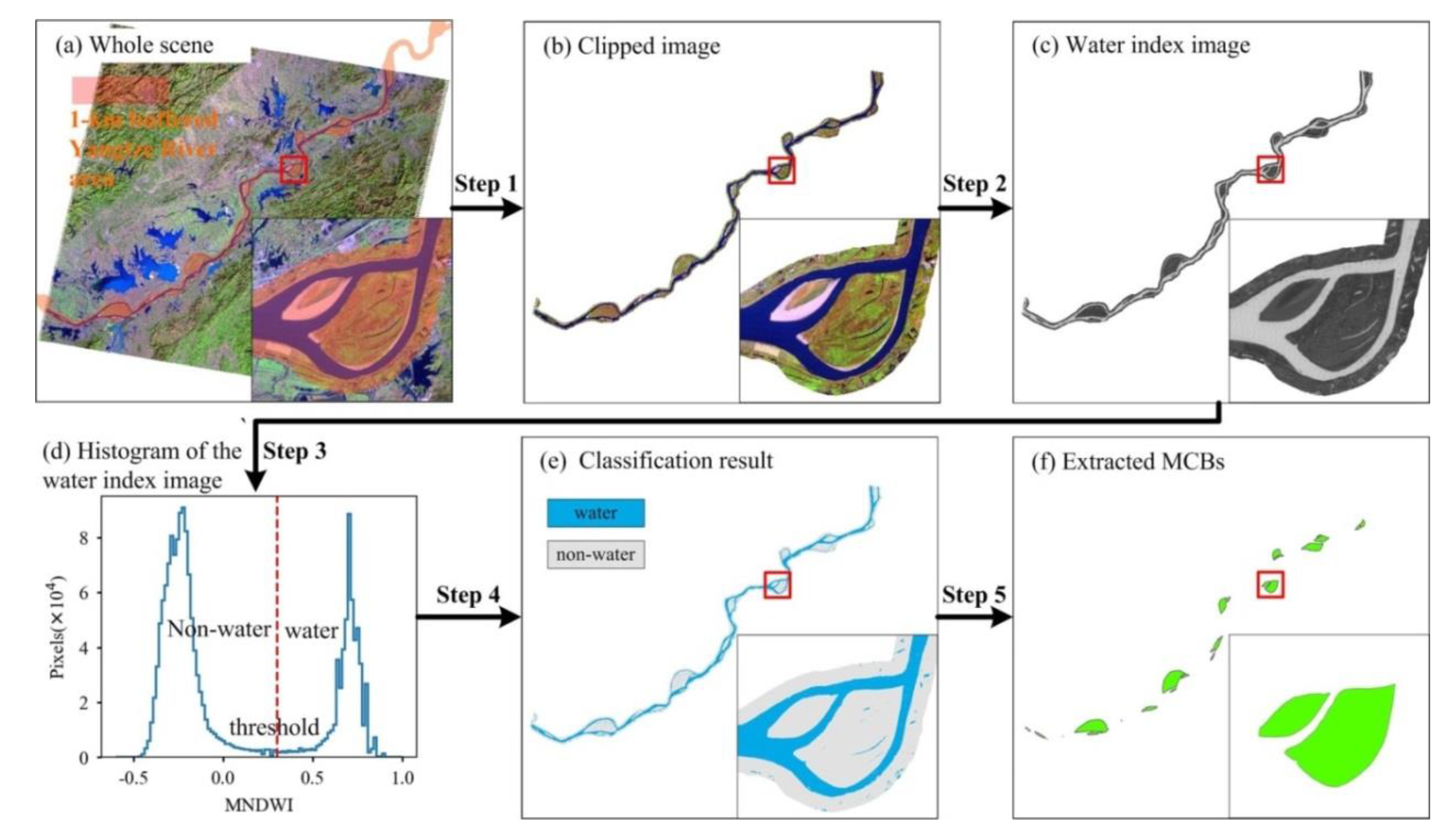
Figure 4.
Accuracy assessment of MCBs for area (a) and LWR index (b).

Figure 5.
Overview patterns of MCBs extracted from Landsat images. Figures (a)-1 and (a)-2 are area histograms of MCBs with consecutive area ranges. (b) Distance-to-TGD histogram of MCBs, and (c) Longitudinal and temporal distribution of all MCBs (each dot represents a single MCB) with different sizes as indicated by their colors. T1, T2, T3, and T4 stand for four different MCB types as explained in Table 2.
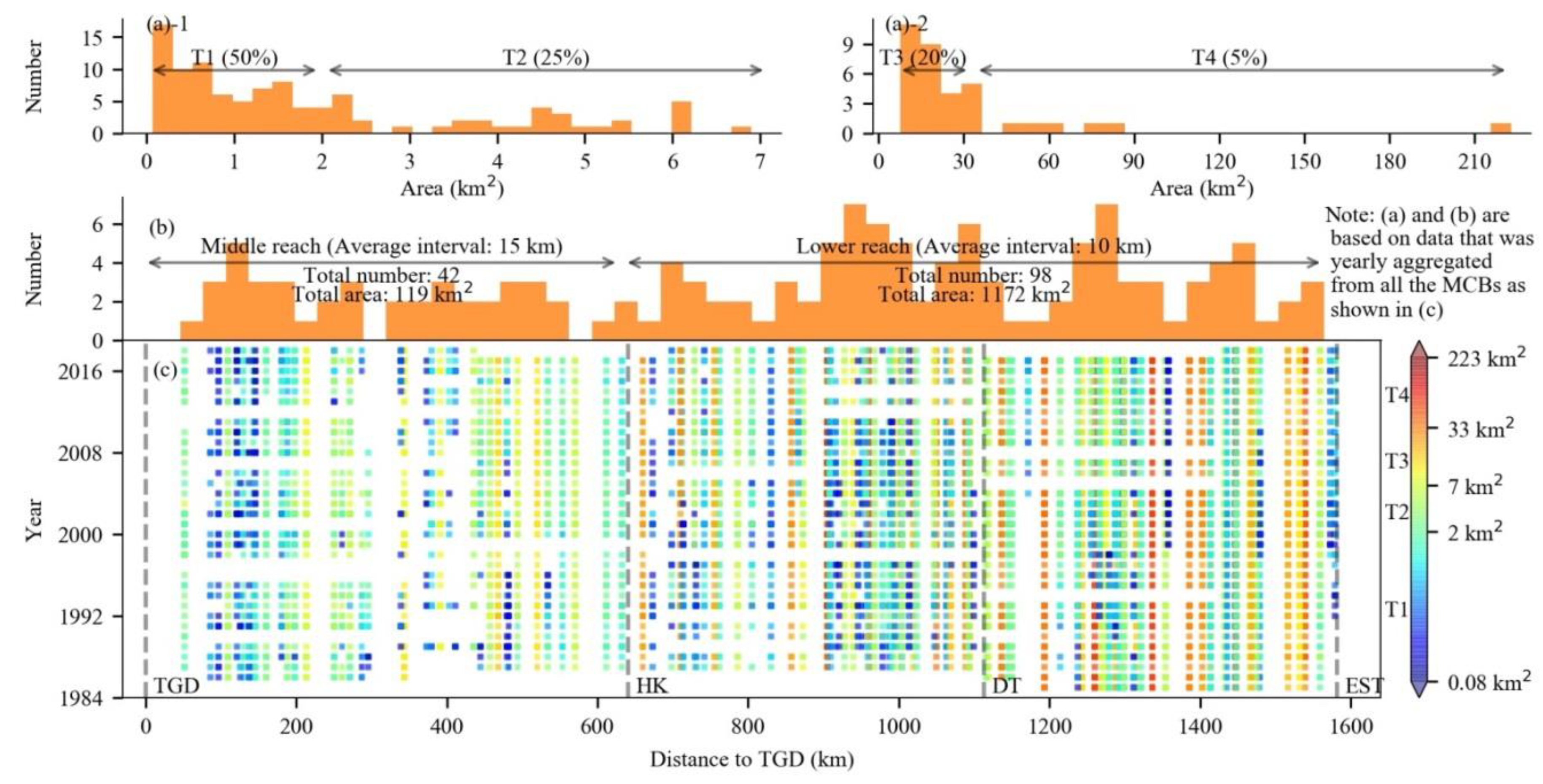
Figure 6.
Longitudinal distribution of MCBs along downstream of TGD in 2016.

Figure 7.
Temporal dynamics of MCB number for different groups of MCBs: (a) Total MCBs, (b) T1 MCBs, (c) T2 MCBs, (d) T3 MCBs, and (e) T4 MCBs. The regression parameters a and R2 stand for regression slope and coefficient of determination, respectively. Slope value with “*” and “**” indicate the corresponding p-value < 0.05 and < 0.01, respectively.
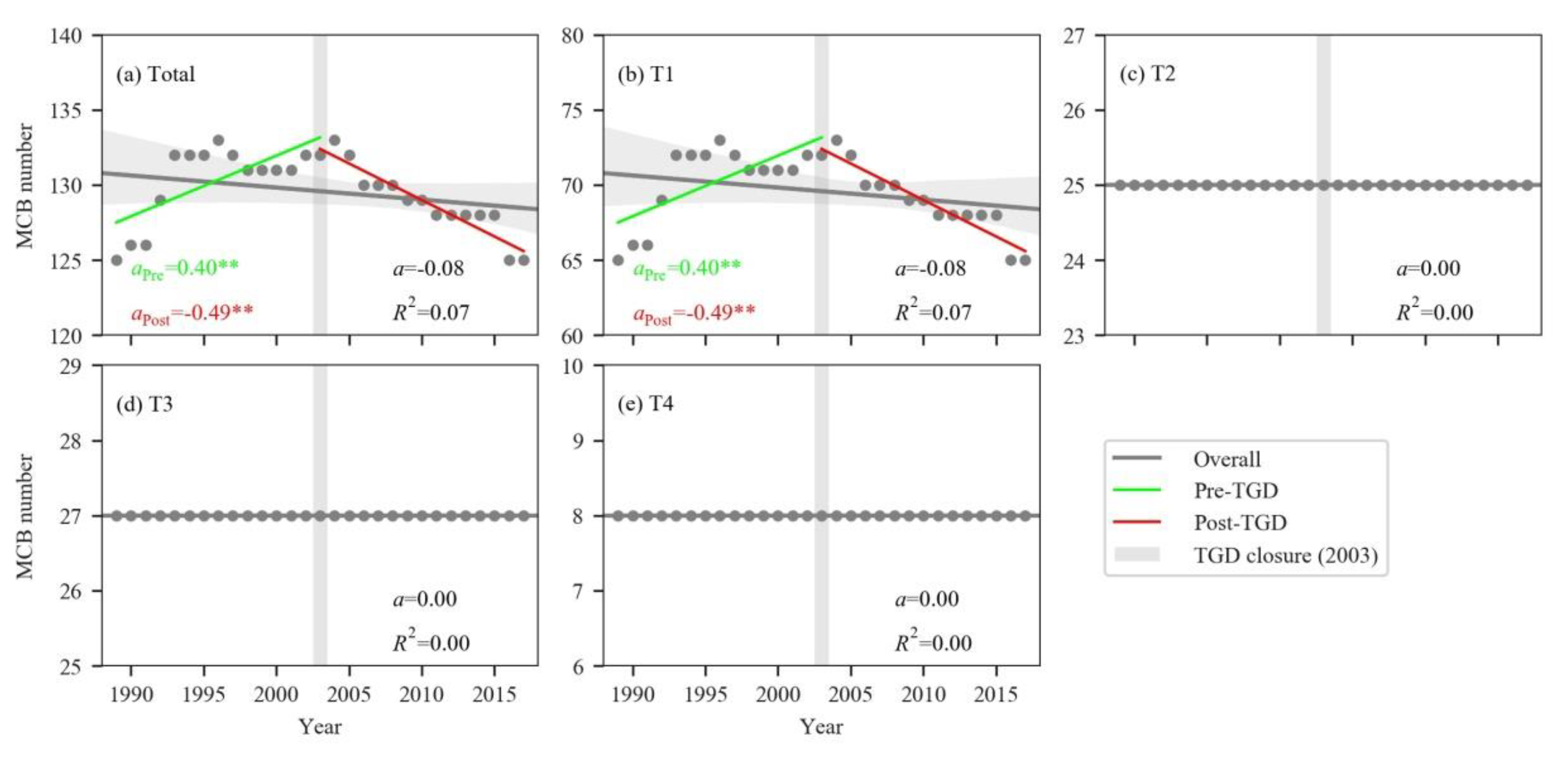
Figure 8.
Longitudinal-temporal distribution of number change events.
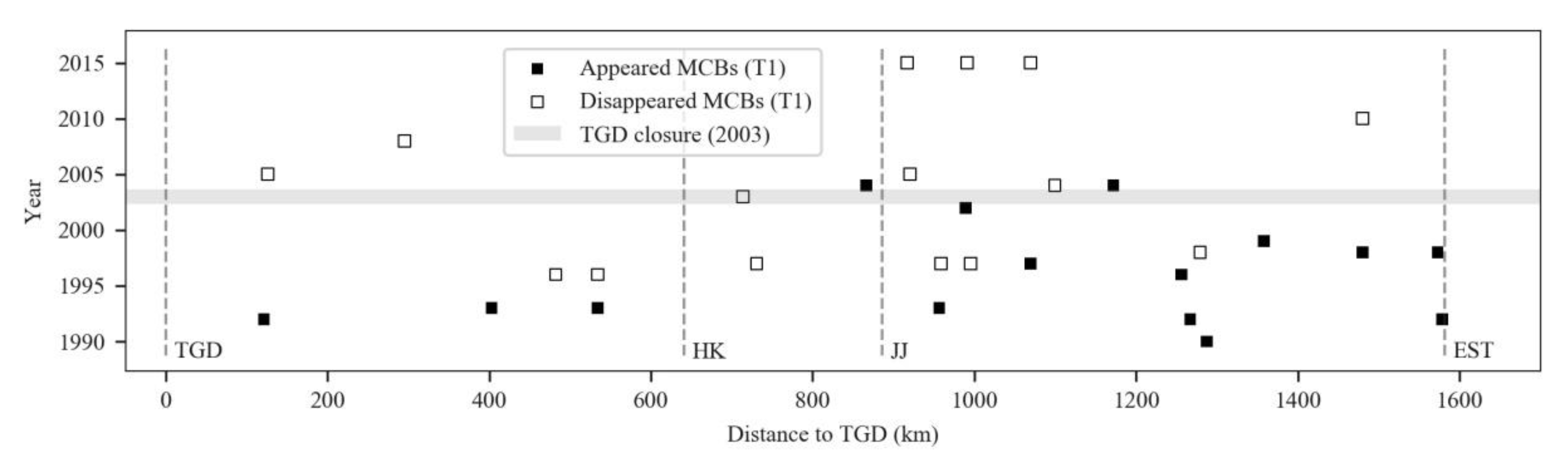
Figure 9.
Area temporal dynamics of different groups of MCBs: (a) Total MCBs, (b) T1 MCBs, (c) T2 MCBs, (d) T3 MCBs, and (e) T4 MCBs. The regression parameters a and R2 stand for regression slope and coefficient of determination. Slope values with “*” and “**” indicate the corresponding p-value < 0.05 and < 0.01, respectively. The CV stands for coefficient of variation which is defined as the ratio of the standard deviation to the mean and here it indicates the extent of variability in relation to the mean area of the MCBs.
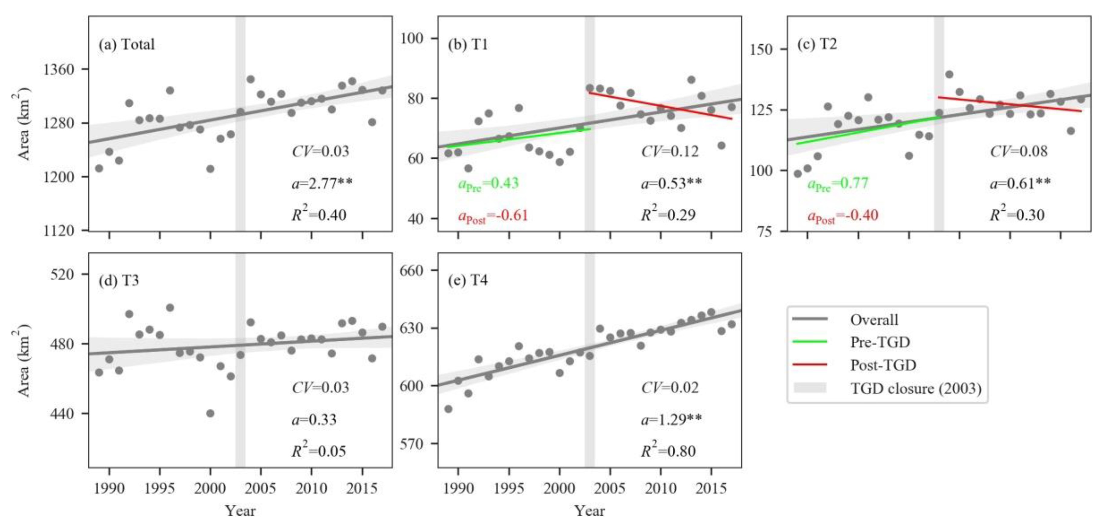
Figure 10.
LWR temporal dynamics of different groups of MCBs: (a) Total MCBs, (b) T1 MCBs, (c) T2 MCBs, (d) T3 MCBs, and (e) T4 MCBs. The regression parameters a and R2 stand for regression slope and coefficient of determination. Slope values with “*” and “**” indicate the corresponding p-value < 0.05 and < 0.01, respectively. Parameter μ stands for the mean value of LWR.

Figure 11.
CV-indicated temporal stability of all individual MCBs changed with their sizes (indicated by log-transformed area) in different periods (overall, pre-TGD, and post-TGD).
Figure 11.
CV-indicated temporal stability of all individual MCBs changed with their sizes (indicated by log-transformed area) in different periods (overall, pre-TGD, and post-TGD).
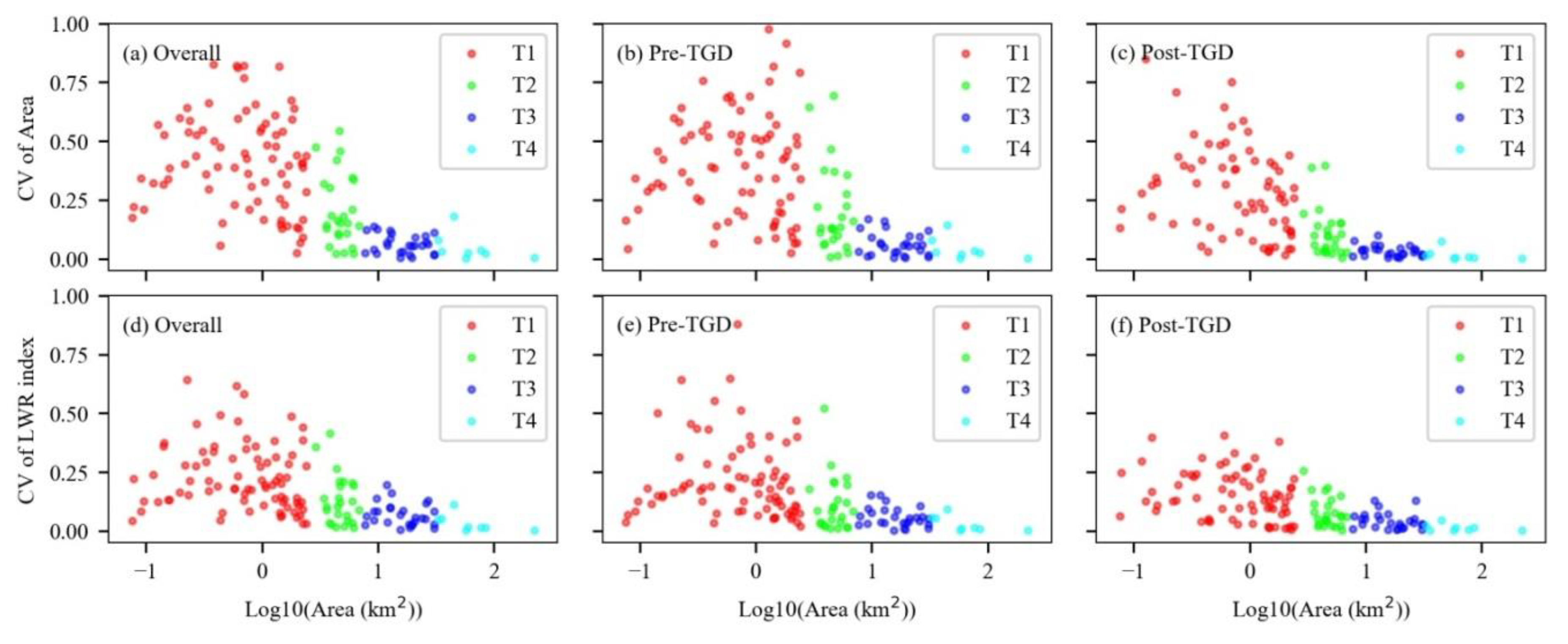
Figure 12.
Flow and sediment regimes in the pre-TGD and post-TGD periods in the three key gauging stations. (a) Annual water discharge from 1985 to 2017, (b) Annual sediment amount from 1985 to 2017, and (c) Monthly averaged water discharge from 1989 to 2002 (Pre-TGD) and from 2003 to 2017 (Post-TGD).
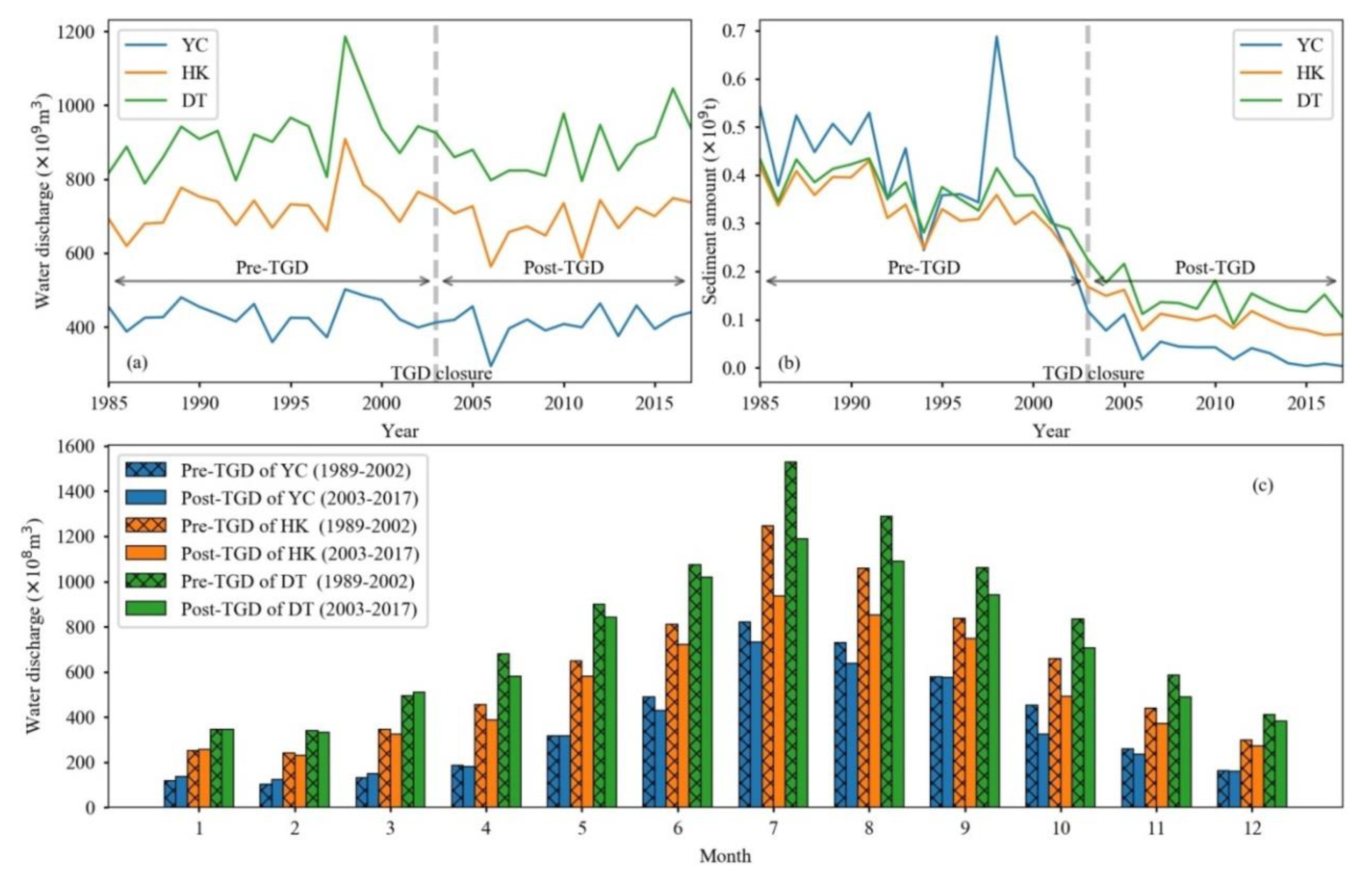
Figure 13.
(a) Frequency of structural changes (FSC) with distance to TGD. (b) The total amount of sand mining in the downstream of TGD.
Figure 13.
(a) Frequency of structural changes (FSC) with distance to TGD. (b) The total amount of sand mining in the downstream of TGD.

Figure 14.
Different structural change types (details can be found in supplementary file Table S2) and their corresponding MCBs numbers for temporal dynamics of (a) area and (b) LWR. For the terms PD, PA, PV, ND, NA, and NV, the first letter “P” or “N” stands for positive trend or negative trend in the pre-TGD period; the second letter “D”, “A” or “R” in each term indicates in a decelerating trend, accelerate, or a reverse trend in the post-TGD period, respectively. For example, “PR” in Figure (a) grouped the MCBs that have a structural change in the area temporal dynamics with positive trend pre-TGD and negative trend post-TGD.


Table 1.
High Spatial Resolution (HSR) images and spatially corresponding Landsat images for accuracy assessment.
Table 1.
High Spatial Resolution (HSR) images and spatially corresponding Landsat images for accuracy assessment.
| HSR Images in Google Earth | Landsat Images | ||||
|---|---|---|---|---|---|
| Source | Acquisition Date | Sensor | Path | Row | Acquisition Date |
| DigitalGlobe | 2010-12-02 | Landsat 5 | 119 | 038 | 2010-12-01 |
| CNES Airbus | 2013-12-10 | Landsat 8 | 119 | 038 | 2013-12-11 |
| DigitalGlobe | 2003-01-04 | Landsat 5 | 120 | 038 | 2003-01-07 |
| CNES Airbus | 2013-11-15 | Landsat 8 | 120 | 038 | 2013-11-20 |
| DigitalGlobe | 2014-11-18 | Landsat 8 | 120 | 038 | 2014-11-16 |
| CNES Airbus | 2017-12-12 | Landsat 8 | 120 | 038 | 2017-12-11 |
| DigitalGlobe | 2008-12-10 | Landsat 5 | 121 | 039 | 2008-12-08 |
| DigitalGlobe | 2015-02-13 | Landsat 8 | 121 | 039 | 2015-02-08 |
| DigitalGlobe | 2017-12-19 | Landsat 8 | 121 | 039 | 2017-12-21 |
| DigitalGlobe | 2017-12-26 | Landsat 8 | 122 | 039 | 2017-12-21 |
| CNES Airbus | 2018-01-11 | Landsat 8 | 122 | 039 | 2018-01-11 |
| DigitalGlobe | 2004-02-13 | Landsat 5 | 123 | 039 | 2004-02-14 |
| DigitalGlobe | 2006-12-19 | Landsat 5 | 123 | 039 | 2006-12-17 |
| DigitalGlobe | 2017-02-16 | Landsat 8 | 123 | 039 | 2017-02-13 |
| CNES Airbus | 2015-01-01 | Landsat 8 | 124 | 039 | 2014-12-31 |
| DigitalGlobe | 2016-12-05 | Landsat 8 | 124 | 039 | 2016-12-08 |
| CNES Airbus | 2017-01-22 | Landsat 8 | 124 | 039 | 2017-01-16 |
| DigitalGlobe | 2017-12-24 | Landsat 8 | 124 | 039 | 2017-12-17 |
| DigitalGlobe | 2018-01-09 | Landsat 8 | 124 | 039 | 2018-01-09 |
Table 2.
Four different types of MCBs.
| Type | Explanation | Area range (km2) | Proportion | |
|---|---|---|---|---|
| Minimum | Maximum | |||
| T1 | Small size | 0.02 a | 2 | 50% |
| T2 | Middle size | 2 | 7 | 25% |
| T3 | Large size | 7 | 33 | 20% |
| T4 | Extra-large size | 33 | 223 b | 5% |
Note: a Only MCBs with their area larger than 0.02 km2 were considered as “true” MCBs as described in Step 5 in extracting MCBs. b 223 km2 was the largest area among the MCBs’ area data.
© 2020 by the authors. Licensee MDPI, Basel, Switzerland. This article is an open access article distributed under the terms and conditions of the Creative Commons Attribution (CC BY) license (http://creativecommons.org/licenses/by/4.0/).
Share and Cite
MDPI and ACS Style
Wen, Z.; Yang, H.; Zhang, C.; Shao, G.; Wu, S. Remotely Sensed Mid-Channel Bar Dynamics in Downstream of the Three Gorges Dam, China. Remote Sens. 2020, 12, 409. https://doi.org/10.3390/rs12030409
AMA Style
Wen Z, Yang H, Zhang C, Shao G, Wu S. Remotely Sensed Mid-Channel Bar Dynamics in Downstream of the Three Gorges Dam, China. Remote Sensing. 2020; 12(3):409. https://doi.org/10.3390/rs12030409
Chicago/Turabian StyleWen, Zhaofei, Hong Yang, Ce Zhang, Guofan Shao, and Shengjun Wu. 2020. "Remotely Sensed Mid-Channel Bar Dynamics in Downstream of the Three Gorges Dam, China" Remote Sensing 12, no. 3: 409. https://doi.org/10.3390/rs12030409
Note that from the first issue of 2016, this journal uses article numbers instead of page numbers. See further details here.