Example of Monte Carlo Method Uncertainty Evaluation for Above-Water Ocean Colour Radiometry
by
 , , , and
Agnieszka Białek
1,* ,
,
Sarah Douglas
1,
Joel Kuusk
2,
Ilmar Ansko
2,
Viktor Vabson
2,
Riho Vendt
2 and
Tânia Casal
3 1
National Physical Laboratory, Teddington TW11 0LW, UK
2
Tartu Observatory, University of Tartu, 61602 Tõravere, Estonia
3
European Space Agency, 2201 AZ Noordwijk, The Netherlands
*
Author to whom correspondence should be addressed.
Remote Sens. 2020, 12(5), 780; https://doi.org/10.3390/rs12050780
Submission received: 27 December 2019
/
Revised: 21 February 2020
/
Accepted: 25 February 2020
/
Published: 29 February 2020
(This article belongs to the Special Issue Fiducial Reference Measurements for Satellite Ocean Colour)
Abstract
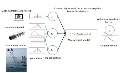
:We describe a method to evaluate an uncertainly budget for the in situ Ocean Colour Radiometric measurements. A Monte Carlo approach is chosen to propagate the measurement uncertainty inputs through the measurements model. The measurement model is designed to address instrument characteristics and uncertainty associated with them. We present the results for a particular example when the radiometers were fully characterised and then use the same data to show a case when such characterisation is missing. This, depending on the measurement and the wavelength, can increase the uncertainty value significantly; for example, the downwelling irradiance at 442.5 nm with fully characterised instruments can reach uncertainty values of 1%, but for the instruments without such characterisation, that value could increase to almost 7%. The uncertainty values presented in this paper are not final, as some of the environmental contributors were not fully evaluated. The main conclusion of this work are the significance of thoughtful instrument characterisation and correction for the most significant uncertainty contributions in order to achieve a lower measurements uncertainty value.
1. Introduction
One of the main successes of the Coastal Zone Color Scanner (CZCS) [1] were the first meaningful ocean colour satellite measurements, particularly considering it was a proof of concept instrument. At the same time, ocean colour measurements have proven to be among the most challenging of all Earth observation measurements. This is due to the small fraction of the ocean related signal that is present in the top of atmosphere satellite readings. An enormous amount of research and measurements went into supporting missions like the Sea-viewing Wide Field-of-view Sensor (SeaWIFS) [2] via the Seventh SeaWiFS Intercalibration Round-Robin Experiment (SIRREX) [3] and the Second Intercomparison and Merger for Interdisciplinary Ocean Studies (SIMBIOS) [4] programs. The second produced further support for many more sensors including for example the Moderate Resolution Imaging Spectrometer (MODIS) [5] and the Medium Resolution Imaging Spectrometer (MERIS) [6]. All that work was summarised in the Ocean Optics Protocols for Satellite Ocean Color Sensor Validation; of particular interest for this study are volumes I to III and VI [7,8,9,10] and a number of publications [11,12,13,14]. All these work stress a particular need for in situ validation and vicarious calibration in ocean colour radiometry (OCR). With the advances in technology and the use of hyperspectral sensors in situ, some aspects of this work need to be repeated. Particularly since significant differences (up to 25%) are found when compared to theoretical modelling and conventional multispectral instruments [15]. It seems that the well known and well characterised multispectral instruments that are described in the NASA protocols are not utilised as much nowadays, as the world focuses on hyperspectal instruments, which provide greater spectral information. However, generally, they are less well characterised but require a wider array of characterisation tests (e.g., spectral stray light). Similarly with the new generation of Ocean Colour sensors like the Sentinel 3 series [16] and planned PACE [17] mission there is a need for even better quality measurements. The old Ocean Colour accuracy requirements, set at 5%, are now being pushed to achieve a level of 3%. In order to achieve this very ambitious target we need to better understand the individual uncertainty components that effect ocean colour measurements as well as their contribution to the final products.
The Fiducial Reference Measurements for Satellite Ocean Colour (FRM4SOC) project, with funding from ESA, aimed to provide support for evaluating and improving the state of the art in satellite ocean colour validation through a series of comparisons under the auspices of the Committee on Earth Observation Satellites (CEOS). The project makes a fundamental contribution to the European system for monitoring the Earth (Copernicus) by ensuring high quality ground-based Fiducial Reference Measurements (FRM) for ocean colour radiometry for use in validation of ocean colour products from missions like Sentinel-3 Ocean Colour and Land Imager (OLCI) [16] and Sentinel-2 Multi Spectral Imager (MSI) [18]. The main aim of FRM4SOC is to establish and maintain SI traceability of ground-based FRM for OCR. Specifically the project develops, documents, implements and reports OCR measurement procedures and protocols. FRM4SOC project activities addressed the SI traceability, comparability and uncertainty evaluation of measurements at several stages of the processing chain. These included comparison of radiance and irradiance sources, that are used for radiometric calibration of the in situ measurement radiometers. Additionally, an indoor comparison of the radiometers took place in controlled laboratory conditions with stable radiance and irradiance sources [19]. The same instruments were taken out of the laboratory to outdoor conditions where they were compared again at two different locations. The first comparison was in Estonia, for measurements of a lake, where the environmental conditions were unfortunately not optimal for above-water radiometry measurements [20]. Nevertheless, this did show the importance of instrument characterisation and the effects due to changeable measurement conditions. The uncertainty budget for the indoor and outdoor exercises were evaluated [20] as relative uncertainty and there was also an attempt to address the variability of the sensors used during the comparisons. The second field comparison was at sea, at the Acqua Alta Oceanographic Tower (AAOT) and used the same instruments. The comparison took place in 2018 and, in this case, the environmental conditions were good.
This paper presents uncertainty budgets for FRM4SOC FRM OCR systems used to validate satellite OCR products. The aim here is to provide an uncertainty budget for in situ ocean colour products. The data used in this evaluation was taken from the second of the above field intercomparison exercises. The instruments selected for this analysis are RAMSES Hyperspectral Radiometers that belong to the University of Tartu. These instruments, in addition to radiometric calibration, had the most optical characterisation tests performed [20]. The characterisation test results were made available for further analysis and allowed correction coefficients to be applied to the data to allow for differences between ideal and non-ideal instrument performance, such as cosine response of a diffuser or detector spectral stray light. In particular, these data enabled the development of a few case studies for uncertainty evaluation with and without corrections applied. The radiometers were used for above-water measurements. Since the FRM4SOC project is intended to be useful for validation of ocean colour satellite products, the hyperspectral results were convoluted with an OLCI spectral band response and thus the results are reported for the Sentinel-3 spectral bands.
The first comparison of OCR measurement at AAOT was performed in 2010 [21] and showed a higher than expected variability of results, often higher than quoted measurements uncertainties. This exercise clearly indicated the need for more frequent comparisons and a more robust measurement uncertainty evaluation. The evaluation of in situ uncertainty is rarely reported, except for the measurement network such as AERONET-OC [22,23]. However, the AERONET instruments are multispectral rather than hyperspectral, which are the most commonly used during validation cruises. Hyperspectral instruments tend to have more instrument characteristics that might affect instrument performance including stray light [24,25] and detector linearity [26], in addition to temperature response [27,28] and cosine diffuser response [29] that are common for both radiometer types. These features of hyperspectral instruments are incorporated into the in situ uncertainty budget presented here. The final products of that evaluation are downwelling irradiance and water-leaving radiance at given viewing configurations, which are all in situ derived quantities. The next step of the in situ data processing leads to remote sensing reflectance or fully normalised water-leaving radiance. This step is not included here, as this is mostly related to the modelling rather than pure measurement errors. We hope to address the next step in future activities, after a number of various models have been used for in situ data modelling, which will allow these methods to be compared and uncertainty results evaluated. The uncertainties are evaluated using the Guide to the expression of Uncertainty in Measurement (GUM) [30] methodology, in particular the Monte Carlo Method (MCM) [31] presented in Supplement 1 to the GUM.
2. Methods
The main purpose of this study is to demonstrate a method of how to determine the uncertainty in downwelling irradiance and water-leaving radiance. Specifically, we investigate two scenarios in which the biases are corrected (the ideal case), and the biases are not corrected but treated as an uncertainty contributor (the non-ideal case). In addition, we present how the non-ideal case shows an under-estimation of measurement uncertainty because the biases are not corrected and the errors due to a lack of that correction are not accounted for. The required data for this activity include downwelling irradiance, downwelling radiance and upwelling radiance as well as all correction factors, the Fresnel reflectance of the water surface, and the fraction of diffuse to direct radiation at the time of measurement. This section provides a description of the lab and field sites and how each parameter was measured, along with how an estimation of uncertainty in the measurement was deduced. Towards the end of the section, the band integration step is described in more detail as is the error correlation. Other effects that have not been taken into account are also described.
2.1. Instruments Used
Three RAMSES instruments (ACC-VIS measuring irradiance and two ARC-VIS measuring radiance) manufactured by TriOS Mess- und Datentechnik GmbH, Rastede, Germany, and supplied by the optical radiometry laboratory of the University of Tartu were used in this activity. The technical parameters are summarised in Table 1.
2.2. Laboratory Calibration
Radiometric calibration, non-linearity, spectral stray light and the cosine correction measurements were performed at a room temperature of (21.5 ± 1.5) °C in a cleanroom equivalent to ISO 14644 Class 8 located at the optical radiometry laboratory of Tartu Observatory, Estonia between 2 and 7 May 2017.
2.3. Field Site AERONET-OC Station
The characterisation of the instruments was carried out as part of the comparison exercise at Lake Kääriku, Estonia. However, due to variable illumination conditions caused by cumulus clouds, few casts were deemed usable and of these, none measured irradiance, upwelling radiance and downwelling radiance simultaneously, hence the decision to use the same instruments at a later campaign site at AAOT near Venice (45.314°N, 12.508°E).
The Aerosol Robotic Network (AERONET) is a system of ground-based sun photometers which support atmospheric studies by providing a readily accessible public domain database of atmospheric properties [32]. The sub network dedicated to Ocean Colour validation is called AERONET-OC [22] and in addition to atmospheric measurements provides water-leaving radiance measurements. The aerosol optical depth, water vapour content and total column ozone values used in this study were measured by the AAOT AERONET-OC station. This is located on the same tower used as the radiance and irradiance measurements (see Figure 1).
2.4. Field Measurements
Two sets of observations of irradiance and radiance were taken at the AAOT, one on the 13 July 2018 between 11:00 and 11:04 (‘cast 1’) and another on the 14 July 2018 between 11:40 and 11:44 local time (‘cast 2’). At these times, downwelling irradiance, downwelling radiance and upwelling radiance were all measured simultaneously. Measurements were performed at the AAOT under near ideal conditions, on the same deployment platform and frame (see Figure 1), under clear sky conditions, sun zenith angles of approximately 24° and moderately low sea state with wind speed of 3.1 m s−1 and 0.5 m s−1 for each cast. The average chlorophyll content was Chl = 0.77 mg m−3 and absorption of the coloured dissolved organic matter was a CDOM (442 nm) = 0.12 m−1.
2.5. Uncertainty Evaluation Methodology
The uncertainties are calculated for the two in situ measurement products: downwelling irradiance, , and water-leaving radiance, that are convoluted to S3 OLCI spectral bands as the final product of interest. The same in situ input data can be used for validation of other satellite sensors as they come from hyperspectral instruments, thus derived radiance and irradiance values can be convoluted with any spectral bands of interest. The wavelength dependence is addressed but omitted in the equations below for better readability. The measurement function for downwelling irradiance is
This measurement equation for downwelling irradiance, , at given Sun zenith angle, is split into two components, one for direct solar irradiance and the other for diffuse sky irradiance. The first term includes the direct-to-total-fraction of irradiance, , the cosine response for direct irradiance, , and the total measured irradiance, , which has already been convolved to OLCI bands and has had various correction factors applied to it. These corrections are further explained in Section 2.5.4. The second term contains, , rather than . is the cosine response correction for the full hemispherical diffuse irradiance. The fraction of direct to total irradiance, , is also shifted to provide the diffuse to total fraction instead. The term 0 is used as a placeholder for any currently undefined model error.
The measurement function for water-leaving radiance is
For water-leaving radiance, , the measurement setup consists of two radiometers, one pointing upwards towards the sky with the zenith angle, and the other downwards towards the water, . They are both at the same azimuth angle i.e., the difference between the sun and the sensor or . The upward-facing instrument measures the downwelling radiance from the sky (marked here with superscript d for downwelling) while the down-facing instrument measures the upwelling radiance from the water (upwelling, u). In the measurement equation, is defined as the upwelling radiance from the water which has had the same corrections factors applied as the downwelling irradiance with the addition of a polarisation correction. Polarisation effects can be assumed to be negligible in irradiance sensors due to their cosine diffuser. The measured values have also been convolved to OLCI bands. , is the equivalent for downwelling radiance. The upwelling radiance includes both light from below the surface (water-leaving radiance) and light which is reflected from the surface of the water. The reflectance of the water is characterised by the Fresnel reflectance, that is a function of the sensor viewing geometry , solar zenith angle, and wind speed, W.
Figure 2 and Figure 3 illustrate the error contributions for the measurement equations for downwelling irradiance and water-leaving radiance respectively. These diagrams were first designed in the Horizon 2020 FIDUCEO project [33] to show the sources of uncertainty from their origin through to the measurement equation. The outer labels describe the effects which cause the corresponding uncertainty.
The colour coding of the error contributions presented in Figure 2 and Figure 3 can be treated as the classification of the errors due to instrument, environment and applied modeling, although that classification in not always straightforward. All yellow highlighted boxes in both figures represent a class of instruments related contributors related to instruments signal, S, absolute radiometric calibration, , and instruments characteristics such as temperature, , detector linearity, , spectral stray light, etc. In addition in Figure 2 pinkish boxes address the errors related to the cosine diffuser angular response. The turquoise box represents the spectral band convolution step, thus this can be classified as modelling class as uses the satellite spectral response function. For the irradiance case the green box represent the fraction of the direct to total irradiance and this is an example where the environmental and modeling errors contributions are tangled together, as some input to the model uses environmental condition such as actual value of AOD (see Section 2.5.10 for more details). Similar situation applies to the red box in Figure 3, for water-leaving radiance to estimate Fresnel reflectance values, this is again a combination of environmental errors such as wind speed and modeling errors that are used to derive this value. Blue box, in both figures, with term represents a placeholder for any other environmental effects that are not fully accounted for in the current version of the uncertainty budget, this can be the structure shadings effect.
2.5.1. Practical Implementation of GUM/MCM
GUM [30] provides a framework for how to determine and express the uncertainty of the measured value of a given quantity which is being measured. The analytical method known as the Law of Propagation of Uncertainties is given by:
where is the combined variance, is the combined standard uncertainty, which is the positive square root of the combined variance, are the sensitivity coefficients of the measurand to the input quantities, , are the uncertainties of the input quantities, are the covariance between input quantities. The covariance between input quantities may be written as,
where is the error-correlation coefficient between and (note: )
The analytical method can become difficult to apply on complex functions with many correlated input parameters where the calculation of sensitivity coefficients is not straightforward. Monte Carlo Methods (MCM) for uncertainty estimation are recognised, accepted and summarised in the GUM supplement [31]. MCM is a numerical method that requires a distinct probability distribution function (PDF) for each of the input components; if input components are correlated, then the joint PDF and the measurement equation are required. The MCM will then run a large number of numerical calculations of the measurement equation, with each iteration using a random choice of each of the inputs from the available range defined by the relevant PDF. The large number of output values calculated using different input values at each iteration provides the uncertainty of the output value with its PDF.
Both methods are allowed in the GUM, with the main document [30] focussing on the use of analytical methods to evaluate the propagation of uncertainty and the MCM (detailed in Supplement 1) [31] using a numerical approach. To evaluate the measurement uncertainty, regardless of the chosen method, several steps need to be taken:
- A measurement function must be defined.
- All sources of uncertainty must be identified.
- Then according to the Law of Propagation of Uncertainty (see Equation (3)) the sensitivity coefficients must be calculated. Nominally, sensitivity coefficients are a partial derivative of a measurement function and a given contributor. For complex functions, it might be impossible to calculate these coefficients analytically. This step is not needed for Monte Carlo approach.
- Using the analytical method, all inputs with non-Gaussian PDFs must be converted to that shape. To do this, divisors are specified for typical shapes. For example, to convert a rectangular PDF to its equivalent in normal distribution, the uncertainty value is divided by . This step is not needed when the MCM is used, as the original PDF can be propagated through the model.
- If any of the input quantities are correlated with each other, an error covariance matrix is necessary (second part of Equation (3)). To combine uncertainties, Equation (3) is used for the analytical approach. In the MCM approach, the measurement function is run many times, each time using randomly selected inputs from previously defined PDFs of the input quantities.
- The results of the analytical approach by default have a Gaussian distribution and when quoted as the output of Equation (3) called the standard uncertainty, which means it has a coverage factor k = 1, or defined as one standard deviation from the mean assuming a normal distribution function. This information expresses the confidence level at 68% that the estimated value is within its quoted uncertainty. The result in the MCM is a PDF of the output quantity and depending on its shape the uncertainty is defined as the standard deviation of this distribution (Gaussian PDF) or by the upper and lower limits that define 68% coverage of that distribution.
- For some applications higher confidence is necessary, and then the standard uncertainty is expanded to k = 2 for 95% coverage or k = 3 for 99% coverage. This is called the expanded uncertainty.
Practical implementation of these steps can vary depending on application. To propagate uncertainty for the measurands of interest for this project ( and ) we propose the following approach:
- All inputs have their standard uncertainty identified in terms of magnitude (value) and PDF shape.
- We handle the correlation between some input quantities (for example, the absolute radiometric calibration coefficients of the different instruments) by treating them as systematic contributions, thus the draws from that distribution are not randomised.
- The final uncertainty value is derived from the resultant PDF.
- All uncertainties are reported with a k = 1 coverage factor.
2.5.2. Error Correlation
A common assumption made during evaluation of measurement uncertainty is the independence of the input components which simplifies Equation (3) to the first term only and leads to the well-known sum of squares expression. However, this might lead to under- or over-estimation of the final uncertainty values if not true.
It might be difficult to evaluate partial error correlation of various components. A practical method to address this is splitting the uncertainty contributors into two categories a) uncorrelated (random) and b) fully correlated (systematic) for which the correlation coefficient is equal to 1.
When applying the MCM using a distribution for a parameter with a particular mean and standard deviation, each draw will be randomly selected. In the case of uncorrelated inputs, all the draws together will make up a PDF with the correct mean and standard deviation. However, it is possible to allow for correlated distributions by selecting identical draws for two or more distributions. It is important to consider this in the MCM since this leads to the correct propagation of systematic errors created by the correlated nature of two parameters.
An obvious example of a systematic error (leading to correlations) is uncertainty in absolute radiometric calibration. For example, in the above-water radiometry situation considered here, the two radiometers that measure radiance are both calibrated against the same radiance source and although the calibration uncertainty has a small contribution from the random errors related to the noise during the measurements, it is dominated by the systematic components related to the radiometric scale realisation; hence the radiometric calibrations are highly correlated. Here, the PDFs representing the radiometric calibration of each instrument should be correlated, meaning the same draws which make up the PDF would be taken for each.
As another example, consider the calculation of the final OCR product for a given OLCI band, in which the values from several pixels are used and convoluted with the OLCI band spectral response function (SRF) to provide the final band integrated value. To avoid underestimation of uncertainty in the integrated value it is necessary to consider if a given uncertainty contributor has a systematic effect on all pixels used for one band.
Each input quantity of the measurement equations is considered whether it is most suitable having a distribution which is assigned as uncorrelated with other distributions or whether the distribution should be correlated with another distribution. For example, for the seven distributions representing the temperature correction in downwelling irradiance (one for each of the seven OLCI bands of interest), each one is correlated with all the others.
2.5.3. Bias Correction
The true value of a measurement can never be exactly known; only an estimate can be made which is as good as the instrument and method used. Therefore, an error (bias) will always exist between the measured and best estimate value.
Another assumption, this time made by the creators of the GUM is that when all identified biases are corrected, only a residual uncertainty in that correction is propagated. In practice, especially for any field measurements, these corrections are not applied and often are unknown.
2.5.4. Data Processing Steps
The processing follows the structure of the measurement equations in Figure 2 and Figure 3. Firstly, all parameters are assigned a PDF and a decision is made over whether any correlation should be assigned for this parameter. Following this, the correction factors (calibration, non-linearity, temperature and stray light and polarisation for radiance only) are applied to the signal. The next step involves a band integration which is performed to convolve the hyperspectral instrument wavelengths with seven OLCI bands. The final step is to calculate the downwelling irradiance and water-leaving radiance respectively using the defined and calculated parameters in the final measurement equations (Equations (1) and (2)). Each PDF is assigned 10,000 draws for this MCM process.
2.5.5. Instrument Signal
The instrument signal is defined as the digital numbers when the sensor is exposed to light conditions () subtracted by the digital numbers in dark conditions (). The RAMSES radiometers do not have a mechanical internal shutter. Instead, black-painted pixels on the photodiode array are used to derive the dark signal and electronical drifts [24]. The values obtained by NPL for further analysis were already converted to radiometric values. Nevertheless, their statistics are used for assessment of the signal uncertainty.
The main steps in defining the PDF for the signal are firstly interpolating the signal to align with OLCI wavelengths and secondly deciding how best to approach the low number of repeated measurements (15 repeats measurements for cast 1 and 12 for cast 2). Here, we consider both procedures.
The three instruments used in this study have a spectral range from 320 to 1050 nm, however for this exercise we are interested in seven OLCI bands (400, 442.5, 490, 560, 665, 778.8, 865 nm) since this procedure is intended to inform comparisons of ground in situ OCR data with satellite sensors. Therefore, the signal is extracted from only the wavelengths overlapping with the OLCI SRF of the seven OLCI bands and then linearly interpolated to match the 200 wavelengths of the OLCI SRF [34] (see Figure 4). There are 200 OLCI SRF values for each band which means the aforementioned signal interpolation to OLCI wavelengths produces 200 values for each repeated measurement. In the next step, the mean of the repeated measurements is calculated for each of the 200 wavelengths, producing 200 signal values per band. These mean values are assigned as the mean of 200 Gaussian distributions which represents the PDF of the signal at each of these wavelengths.
Later in the processing, once all parameters have been defined, the band integration step, described in Section 2.5.14, convolves these values with the OLCI bands to produce one value per band for .
The readings taken for and only covered a 5-min window, meaning only 15 repeat measurements were taken for cast 1 and 12 repeats for cast 2. This is a very small number of repeated measurements and is far from enough to get a representative mean and standard deviation of the measurements. Since there is not a smooth distribution, it is difficult to decide whether to use the mean, median or mode of the repeated measurements. In this study, the typical standard uncertainty of the mean formula is used Equation (5). Additionally, the mean of the repeated measurements is chosen for the PDF.
where u is the uncertainty, N is the number of repeat measurements and is the standard deviation of light values.
2.5.6. Calibration Coefficients
The calibration of each instrument was performed in the optical radiometry laboratory at University of Tartu. The calibration coefficients and associated uncertainty values are incorporated into the Monte Carlo analysis by appropriate PDF. The instrument readings are automatically adjusted for the calibration coefficients, thus in the MCM, the PDF is taken to be a Gaussian distribution with mean equal to 1. The standard deviation is equal to the standard uncertainty associated with the calibration. These values are presented in Table A1 in the Appendix A.
2.5.7. Non-Linearity Correction
The integration time used when capturing the measured spectra can lead to non-linearity effects in the results. The maximum value of non-linearity effects was determined in the indoor calibration for the two radiance instruments, but not for the irradiance instrument [20]. As the principal aim of this study is to outline the method and only secondary provide results, the radiance instrument corrections are used for the irradiance instrument. The non-linearity correction values are provided for all instrument wavelengths. Similarly, to the instrument signal, in order to align with the OLCI bands, the only non-linearity values used are those whose wavelengths overlap with the SRFs of each of the seven OLCI bands. These are then interpolated to match the 200 OLCI SRF wavelengths. The interpolation method chosen was linear interpolation due to the smoothness of the non-linearity correction curve (see Figure 5).
Each of the 200 resultant non-linearity correction values is assigned a PDF, which is a rectangular distribution with a mean value of 1 and half-width equal to the linearity correction value.
Note that the detector might and often does exhibit non-linearity due to the radiance flux levels as well as integration time [26], however tests showing these effects were not used in this study.
2.5.8. Temperature Correction
The variation of the instrumental calibration coefficients due to temperature is based on a previous evaluation [27] presented in Figure 6. The variability in % at the seven central wavelengths of the bands of interest (400, 442.5, 490, 560, 665, 778.8, 865 nm) were selected. The seven PDFs which represent the temperature correction at each band were defined to be Gaussian distributions with a mean value of 1 and a standard deviation equal to the aforementioned variability. The standard deviation values are presented in Table A1 in the Appendix A.
2.5.9. Stray Light Correction
Scattering or reflections in the radiometer optics cause light from one part of the spectrum to fall on pixels associated with light from another part of the spectrum. This effect is known as spectral stray light and is common in hyperspectral instruments and must be corrected for.
This study was intentionally planned so that all instruments would be well characterised, whereas typical campaigns have much less information about the instrument performance, including the stray light characterisation. Hence, we consider two scenarios for the stray light. The first case is for an ideal situation in which the stray light is corrected for based on the performed characterisation and we assign an uncertainty to this method as described in point (i) below; the second, non-ideal, case does not correct for stray light and instead we demonstrate the scale of uncertainty which will result from this in point (ii).
(i) The stray light characterisation provides correction values for each of the instrument wavelengths (see Figure 7). The correction values obtained are quite erratic. Due to the correction values being low in magnitude, it is possible that the erratic behaviour could be due to noise from the stray light measurement.
The stray light correction values used were calculated by convoluting the stray light values with the OLCI SRF [34]. The selected values are presented in Figure 7 as the green cross series.
For the ideal case, the PDFs assigned for stray light for each band is a Gaussian distribution with a mean equal to the stray light correction acquired from the polynomial. The stray light characterisation does have an uncertainty associated with it, but this is unknown. A value of 5% is chosen which accommodates for the true uncertainty and is negligible in comparison to the assigned uncertainty of other variables [20], meaning that the quantity will have little or no effect on the further results.
(ii) For the non-ideal case, no correction is applied. The assigned distribution is a Gaussian distribution with mean equal to 1 and standard deviation equal to the fitted polynomial stray light correction (see Figure 7 and Table 2) at the seven OLCI bands of interest.
The total uncertainty from this method will also need to take into account the difference the lack of correction makes in the value of the downwelling irradiance, and water-leaving radiance, .
Section 3 gives an overview of the impact of both of the above scenarios.
2.5.10. The Fraction of Direct to Total Irradiance
The fraction of direct to total irradiance is applicable to downwelling irradiance measurements only and can be estimated using measurements of the aerosol optical depth, water vapour content and total column ozone in a radiative transfer model. This takes into account the atmospheric transmission of radiation for the conditions specified. In this study, an AERONET-OC [22] station at the observation site provided the atmospheric conditions at the time of data acquisition, and then the radiative transfer model, 6S [35], was used to estimate the direct to total ratio. The atmospheric parameters for both casts were AOD at 500 nm 0.112 and 0.297, precipitable water in 2.83 cm and 3.13 cm, and ozone 330.1 DU and 329.5 DU. The uncertainty components of consist of i) the accuracy of the 6S radiative transfer model, ii) the uncertainty of the inputs to 6S and iii) an error related to the designated atmosphere type.
(i) The 6S does not provide an estimate of its own accuracy, however a comparison of 6S with a highly accurate Monte Carlo radiative transfer yielded a maximum observed relative difference between the two methods of 0.79 % for a maritime atmosphere [36]. This value is used as an estimate of 6S uncertainty and is shown as “6S model accuracy” row in Table 3.
(ii) There are several inputs of the AERONET data to 6S, namely aerosol optical depth (AOD) at 550 nm, precipitable water and total column ozone. The only of the three variables which causes a change in is the AOD at 550 nm. Therefore, the only variable which we need to consider the uncertainty of is AOD at 550 nm which has an uncertainty of 0.01 according to [32]. The sensitivity of the resultant in 6S with a change of in AOD has been calculated. The difference observed makes up the corresponding uncertainty values shown in the rows labelled “AOD 550 nm” in Table 3.
(iii) The AAOT site is eight nautical miles from the coast of Venice and as such the atmosphere is between continental and maritime and should possibly be considered coastal. However, the 6S model has several defined atmospheres for the user to select which does not include coastal, hence for this study the ‘maritime’ option will be used and the error in this assumption will be estimated by comparing the results of both ‘maritime’ and ‘continental’. The differences between the two atmospheric types varies across wavelengths, hence the uncertainty due to this will also be wavelength dependent (see the row labelled “Atmosphere type assumptions” Table 3).
Assuming that each contributor is independent, using the Law of Propagation of Uncertainties, we can calculate the uncertainty of (see Table 3). This uncertainty is applied as half the width of a rectangular distribution centred on a mean value of 1. Note that, here we assume Table 3 shows the uncertainty in terms of the width of a rectangular PDF, whereas in further processing this uncertainty is used as the standard deviation of the Gaussian PDF (see Figure 10 where the values used in MCM are quoted). This means that the values for are not equal since the standard deviation of a rectangular distribution is smaller than half the width of a rectangular distribution.
2.5.11. Cosine Response ( and )
These two components are applicable to downwelling irradiance measurements only. To capture irradiance over a full hemisphere, instruments are equipped with cosine diffusers which collect radiances from the hemisphere and transmit them onto the radiometer. The ideal diffuser will transmit light in proportion with the cosine of the incident angle. However, instruments always differ from the theoretical ideal, hence the need for this to be characterised and corrected for, meaning the residual elements of uncertainty depend on the correction method.
Downwelling irradiance is made up of two components: direct sun irradiance and diffuse sky irradiance. These components are not affected the same way by a non-perfect cosine response and so are separated in the measurement equation. The cosine response term, , incorporates only the direct solar component thus relates to SZA during the measurement and the error in cosine response diffuser for this particular angle. Whereas, , the cosine response over the full hemisphere, integrates the diffuse light component across the hemisphere, and integrates the deviation from the perfect diffuser across the whole hemisphere as well.
In this study, the cosine response has been fully characterised with four repeated measurements and is propagated as the ideal case below (i). However, often the cosine response is unknown and thus not corrected for. This section demonstrates the impact of an additional scenario (ii), in which the only information known about the cosine response is the manufacturer’s quote of the uncertainty due to the cosine response. Here we choose the value of 3% as this is similar to the cosine response error in this study for all bands and is also a typical value quoted by manufacturers for angles under 60° [37].
The ideal case is having the cosine response errors for a range of solar zenith angles and wavelengths. In this study, the diffuser was characterised in Tartu Observatory before the field comparison in May 2017 for 45 angles across the hemisphere and seven wavelengths. Figure 8 shows the results of the laboratory test for the instruments used in this study. The average of the four repeated measurements was linearly interpolated to the solar zenith angle and the central wavelength of each of the seven bands of interest. The cosine response correction is treated as a Gaussian distribution centred on the interpolated value. The standard deviation of this distribution is assigned from the standard deviation of the four repeated measurements.
The non-ideal case examines the typical scenario in which a manufacturer has quoted the cosine response to be equal to 3% with no additional information. Typically, this is assigned as the standard deviation of a Gaussian PDF of mean 1 (i.e., no correction is applied, just an uncertainty). However, the cosine response is a systematic error and should shift the mean value of as in the ideal scenario (i), but this will not happen if parameterised as a PDF of mean 1 hence the mean value is incorrect. This should be accounted for by applying an additional measure of uncertainty based on the impact not accounting for the bias has on .
The diffuse component requires all cosine responses to be integrated over the hemisphere. Assuming an isotropic sky radiance distribution, this is calculated using:
where is the integrated cosine response over the full hemisphere, and is the cosine response for a given illumination angle. We again look at two similar scenarios, the ideal case (i) demonstrates a scenario in which all cosine response errors are known, and the non-ideal (ii) demonstrates a situation where the only information known regarding the response is that it is within 3% for angles and 10% for angles . No values were provided by the manufacturer in this study, but these values are typical for manufacturers (e.g., Sea-Bird Scientific HyperOCR radiometer [37]).
The isotropic sky is a simplification and clear-sky radiance distributions are not isotropic and normally show larger radiances for large zenith angles (e.g., [38]) and band circumsolar brightening (aureole) [39]. For measurements presented here with SZA approximatetly 24° the aureole effect is minimised by the small errors in cosine response of the diffuser for small incidence angles (see Figure 8). For the horizon brightening the factor in Equation (6) would however minimize their contribution to . The diffuse component of the downwelling irradiance for clear skies is about 40-30 % for short wavelengths and decreases at longer wavelengths (see Table 3 for the actual values observed during the field measurements), further reducing the impact of on the uncertainty evaluation. Obviously, the situation is different for hazier skies, or for high values of the solar zenith angle, which anyway are not recommended conditions for the satellite validation activities.
For the ideal case, the cosine response values are corrected for by taking an average over the four repeated measurements for at each angle and each wavelength. Then these can be integrated over all angles and interpolated to the wavelength of interest. The PDF assigned for the diffuse component is a Gaussian distribution with mean equal to these integrated cosine values and standard deviation originating from the standard deviation of the four repeated measurements of the cosine response.
The non-ideal case does not correct for the cosine response, therefore the mean of the Gaussian distribution is equal to 1 and the standard deviation relates to 3% for angles and 10% for angles (which are typical values for manufacturers (e.g., Sea-Bird Scientific HyperOCR radiometer [37]). However, the cosine response is a systematic error which should be corrected for, hence an additional measure of uncertainty must be applied to take into account the lack of completing a correction. This is equal to the difference in the mean values of the resultant calculated with and without a correction applied (i.e., the difference between the resultant from the ideal and non-ideal cases).
2.5.12. Polarisation Correction
Polarisation effects can be assumed to be negligible in irradiance sensors due to their use of a cosine diffuser that acts as a scrambler. However, polarisation is an important correction for radiance sensors.
The sensitivity of the instrument to the polarisation of light was not determined during the outdoor inter-comparisons and so instead the worst-case data from [40] was used. This data was used as a measure of uncertainty of the values, rather than used as a correction. Hence, the mean of the polarisation distribution is equal to 1 and standard deviation derived from [40] (see Table A1 in the Appendix A for the values of polarisation used).
2.5.13. Fresnel Reflectance
The Fresnel reflectance values for each cast were calculated at the AAOT field site based on approach proposed by Ruddick [41,42] that goes back to Mobley [43] and related Hydrolight simulation, the correction takes into account the wave height by using the wind speed as input factor. The values are 0.0258 and 0.0271 for cast 1 and 2 respectively. Just one value was used across all wavelengths for each cast, which is not ideal. The uncertainty of the reflectivity has previously been determined by [43] at the AAOT site for wavelengths 412, 443, 488, 551 and 667 nm. These values have been interpolated to the wavelengths of interest in this study and are presented in Table A1 in the Appendix A.
2.5.14. Band integration
In order to compare the ground-based in situ ocean colour data with the satellite sensor, OLCI, the hyperspectral instrument must be convolved with OLCI’s SRF [34]. For this, we use the following equations.
The weight factors for each wavelength are:
where n is the interpolated wavelength, is the SRF of a band, and is the normalized weight coefficient for the n’th wavelength. The summation of the term is the summation of the SRF values over the 200 wavelengths in one band. The irradiance/radiance value for the corresponding OLCI channel is calculated as:
where denotes the irradiance/radiance which has had the correction factors applied ( or ) at the n’th wavelength.
The two inputs to this band integration are and . The former is calculated from applying the correction factors to irradiance/radiance and interpolating the values to match the 200 SRF wavelengths (see Section 2.5.5). The latter is composed of the SRF of OLCI published by ESA [34]. This has a Gaussian PDF of mean equal to the SRF and standard deviation calculated from guideline SRF relative accuracy for OLCI [44]. The accuracy has been interpolated to match each of the 200 wavelengths in the OLCI SRF. Each of the wavelengths for each band is assigned a PDF for .
For the first wavelength of the first band, a PDF for will first be assigned. Then a summation over all 200 wavelengths in that band will occur which can be used to determine . This is then multiplied by the first of the 200 values of . The result is stored waiting for the result of the next iteration to be added. This procedure occurs for each of the 200 wavelengths in the first band at which point the value of for the first band has been determined.
This process is then repeated for each of the seven OLCI bands yielding the seven values for which can then be applied to the measurement equations to find the downwelling irradiance or water-leaving radiance.
2.5.15. Error Correlation Summary
Below we summarise all uncertainty contributors that have correlated errors. Please note that the correlation can be between different levels. For example: correlation can exist between all pixels in a given band, or between two different instruments. We do not include correlation between bands in this study.
The parameters which are considered to have correlated errors are listed below, together with the approach used to allow for these correlations in the uncertainty evaluation:
There is a different set of PDFs and draws for each OLCI band, but within the band the 200 contributing wavelengths are correlated with each other. For the radiance case, the same PDFs and draws for each band are used for both instruments (i.e., the instruments are correlated with each other).
There is one set of draws for all OLCI bands, but each band has an individual PDF (i.e., the mean and standard deviation for each band differs but the draws are identical).
There is a different set of PDFs and draws for each OLCI band; but within the band the 200 contributing wavelengths are correlated with each other. For the radiance case, different PDFs and draws are used for each instrument.
Different set of PDFs draws for each OLCI band, but within the band the 200 contributing wavelengths are correlated. For radiance case different PDFs and draws are used for each instrument.
2.5.16. Effects Not Accounted for
So far in this paper, we have not mentioned environmental effects, such as those caused by waves, shadows and sun glint, which may cause systematic variations in the signal which propagate through to the resultant radiance. No additional information was available about the field campaign and so we neglect these terms here. In a number of cases, interpolation has been used to estimate a variable for the wavelengths of interest. The use of interpolation does need to be accommodated for in the MCM with an uncertainty. However, here the uncertainty will be negligible as compared to the other factors, hence it is omitted from our method.
3. Results
This section presents the outputs of the uncertainty analysis for the ideal and non-ideal cases, as well as a corrected case where an extra correction is applied to show the true resultant uncertainty when not corrected. The MCM for downwelling irradiance and water-leaving radiance was run over two casts and results are presented for the seven OLCI bands of interest (400, 442.5, 490, 560, 665, 778.8, 865 nm).
3.1. Downwelling Irradiance
The ideal scenario relates to the case in which the cosine correction and stray light were well characterised and were corrected for. As previously mentioned, the MCM requires each parameter in the measurement equations to be assigned a PDF based on collected data, or best knowledge, etc. These distributions as shown in Figure 9 were then propagated through the measurement equation to find the downwelling irradiance, .
Figure 10 presents the summary values of the MCM simulation for cast 1. The value of several of the variables (S, , , ) is chosen for just one wavelength out of 200. Most of these variables vary over the 200 wavelengths. Here we present the 99 value as an example for reference. In the calculations, all 200 values are propagated.
The quoted number of significant figures exceeds the number which are conventionally quoted because the values are intended to be compared with values in the other figures and tables of the report. The final values which are quoted in Section 4 are in line with standard significant figure reporting.
The results for the cases in which neither stray light nor the cosine error are corrected for look different (the two bottom panels in Figure 10) they were each assigned a mean value of 1 and an uncertainty relating to typical manufacturers’ estimates (cosine) and the correction itself (stray light). It is possible to see the effects of stray light and the cosine error separately since each parameter exists in separate parts of the measurement equation. For example, it is clear that the mean of is set to 1 and the standard deviation is much higher in the non-ideal case than ideal. Additionally, the changes in parameters can be tracked through up to . Beyond this, the correction is mixed with the cosine correction which can be seen to dominate the standard deviation of the majority of bands of .
The uncertainty presented in the lower panel of Figure 10 is an under-representation of the true uncertainty that is applicable when corrections are not applied. This is because we have taken into account the uncertainty in the measurement but have not accounted for the lack of correction.
Hence, we add the bias which is the difference between the ideal mean value and the non-ideal mean value (see Equation (9)) and add this to the standard deviation of the non-ideal case.
The result is illustrated in Figure 11 as the “Corrected non-ideal” case. This exhibits a much wider standard deviation, which is the true standard deviation which should be used but cannot be calculated without the ideal characterisation.
Table 4 provides an overview of the values of interest in this correction. The mean values of the PDF function obtained in the MCM processing for downwelling irradiance are shown for the ideal and non ideal case in irradiance units (column 2 and 3 in the Table 4). Column 4 contains the bias values, thus the difference between the two means calculated according to the Equation (9). The columns 5 to 7 present relative standard uncertainties for the three different scenarios.
3.2. Water-Leaving Radiance
The same approach as for the downelling irradiance case is used to present, in Figure 12, the water-leaving radiance results. The value of several of the variables (, , , , , , , , ) presented in Figure 12 is chosen for just one wavelength out of 200. Most of these variables vary over the 200 wavelengths. Here we present the 99 value as an example for reference. In the calculations, all 200 values are propagated.
The ideal scenario relates to the case in which stray light was well characterised and corrected for as is explained thoroughly in Section 2.5.9. For the non-ideal scenario stray light is not corrected for and was assigned a mean value of 1 (i.e., no correction applied) and an uncertainty relating to the previously used correction values. From Figure 12 it is clear that the mean of the stray light correction factors is 1 and the standard deviation is larger as compared to the ideal case. These changes can be seen to affect downstream parameters in the measurement equation.
The 778.8 nm and 865 nm bands resulted in a negative water-leaving radiance. A negative value here is not theoretically possible, so is likely due to an error in the measurement model. However, we do not expect to observe any water-leaving radiance measurable with the used radiometers at AAOT for these wavelengths. We quote the water leaving radiance as 0 with no meaningful uncertainty.
The uncertainty for non-ideal case is an under-representation of the true uncertainty that is applicable when corrections are not applied. This is because we have taken into account the uncertainty in the measurement but have not accounted for the lack of correction. Hence, we add the difference between the ideal mean value and the non-ideal mean value and add this to the standard deviation of the non-ideal case. This exhibits a much wider standard deviation, which is the true standard deviation which should be used but cannot be calculated without the ideal characterisation. Table 5 provides an overview of the values of interest in this correction. The mean values of the PDF function obtained in the MCM processing for water-leaving radiance are shown for the ideal and non ideal case in radiance units (column 2 and 3 in the Table 5). Column 4 contains the bias values, thus the difference between the two means calculated according to the Equation (9). The columns 5 to 7 present relative standard uncertainties for the three different scenarios.
4. Discussion
This paper presents an evaluation of an uncertainty budget for above-water OCR measurements performed as part of FRM4SOC field inter-comparison exercise which demonstrates the importance of correcting for instrumental biases. The data from one participant (University of Tartu) were used here for further investigations. These radiometers were chosen because the radiometers, in addition to radiometric calibration, had a set of optical characterisations completed. This enabled an investigation of different scenarios, where we correct the measurand for the known instruments’ characteristic (we call this the ideal case). Since having this set of optical characterisations is rather rare, we present a so-called non-ideal case, where the biases caused by instrument characteristics are not corrected for. The most important case is, however, the corrected non-ideal scenario where we evaluate the real uncertainty related to the uncorrected bias case.
We presented the measurement equations using uncertainty tree diagrams that in graphical form show all the relationships between different uncertainty contributors. The uncertainty was evaluated by assigning PDFs to each contributor and propagating this through the measurement equations using the MCM method.
To test the stability of the model, the MCM was run 15 times for both the irradiance and radiance ideal cases. The standard deviation of the standard uncertainty of and are shown in Table 6.
The variability in the uncertainty of and allow an estimate of the number of significant figures to be quoted. The final standard uncertainty values are quoted to two significant figures as shown in Table 7. It is important to note that components related to environmental conditions such as structure shading, sun and sky glint, wave focusing etc are not included in this uncertainty budget, therefore the true uncertainty value is likely to be higher.
The fully evaluated uncertainty values as presented in Table 7 are potentially higher than expected, commonly agreed or used, especially for the downwelling irradiance, are caused by the biases due to non-perfect cosine diffuser response and stray light added to the uncertainty estimate. We evaluate the biases as the measurement uncertainty during AAOT field inter-comparisons for one participant’s radiometers as the results provided for the comparison pilot were not corrected for any of the instruments’ characteristics. When these biases are treated not as errors but as uncertainty components, firstly the final product mean value is incorrect since no correction takes place. Secondly, the uncertainty associated with that value is underestimated (see Figure 11). This is because the uncertainty in the measurement has been accounted for (typical manufacturers’ estimates are used for the cosine error and the correction itself for stray light) but not the lack of correction. Hence the need to find the difference between the ideal mean value and the non-ideal mean value and add this to the standard uncertainty of the non-ideal case, producing the results of the corrected non-ideal scenario.
We chose to correct only the cosine diffuser and stray light characterisations to present the three scenarios (ideal, non-ideal and corrected non-ideal). However, in practice, any parameter which is the dominant source of uncertainty and can be feasibly corrected should be corrected for. Once that parameter has been corrected for, the next most dominant should also be considered, and so on. The limiting factor in this step-wise procedure is the absolute calibration which cannot be corrected for. Hence any parameters with an uncertainty less than that of the absolute calibration does not need to be corrected for. For example, looking at Figure 10 and Figure 12 that show the magnitude of uncertainty contributors, one could recommend that any component with uncertainty greater than should be corrected for. This would include three of the bands of both temperature and linearity for and similar for .
In this study, the environmental uncertainty is not considered, but this may be the limiting factor since it is likely to be larger than the absolute calibration uncertainty. An evaluation of how to correctly estimate environmental uncertainty for a range of conditions is yet to be completed.
We presented the MCM to evaluate uncertainty as we found it simpler to apply especially for the hyperspectral data that require band integration to fit the satellite bands. However, the equation for (see Equation (A1)) leads itself to being a good example to show the traditional Law of Propagation of Uncertainties defined in GUM [30]. Appendix B presents a comparison of MCM to correctly applied analytical method and a case where the so-called sum of squares does not work.
5. Conclusions
This study has demonstrated how to conduct an uncertainty analysis for in situ radiometers of Ocean Colour measurements. The results of the three scenarios (ideal, non-ideal and corrected non-ideal) in Table 4 and Table 5 highlight the importance and benefits of carrying out instrument characterisations before campaigns and performing instrument corrections in addition to absolute radiometric calibration. It is recommended that the sources of uncertainty which are likely to dominate over the absolute calibration uncertainty (or other more dominant uncertainty contributors which cannot be corrected for) should be characterised before campaigns so that these can be corrected for. This will produce results with reduced uncertainties as demonstrated in the ideal scenario (Table 4 and Table 5). The most likely parameters which will need prior characterisations are stray light, cosine, temperature and non-linearity corrections. Following these guidelines will support compliance with the requirements of in situ Ocean Colour measurements for use in satellite product validation.
Author Contributions
Conceptualization, A.B.; methodology, A.B.; software, S.D.; validation, A.B., S.D.; data curation, J.K., I.A., V.V.; writing—original draft preparation, A.B., S.D.; writing—review and editing, A.B., J.K., V.V., R.V. and T.C.; visualization, S.D.; project administration, R.V. and T.C. All authors have read and agreed to the published version of the manuscript.
Funding
This work was funded by European Space Agency project Fiducial Reference Measurements for Satellite Ocean Colour (FRM4SOC), contract no. 4000117454/16/I-Sbo.
Conflicts of Interest
The authors declare no conflict of interest.
Appendix A. Uncertainty Values

Table A1.
The mean and uncertainty values used for each parameter for the radiance simulation.
| Wavelength (nm) | 400 | 442.5 | 490 | 560 | 665 | 778.8 | 865 | |
|---|---|---|---|---|---|---|---|---|
| Calibration | Mean | 1 | 1 | 1 | 1 | 1 | 1 | 1 |
| Std (%) | 1.2 | 0.78 | 0.76 | 0.73 | 0.71 | 0.73 | 1.35 | |
| Temperature | Mean | 1 | 1 | 1 | 1 | 1 | 1 | 1 |
| Std (%) | 0.2 | 0.2 | 0.2 | 0.3 | 0.7 | 1.3 | 2.7 | |
| Polarisation, | Mean | 1 | 1 | 1 | 1 | 1 | 1 | 1 |
| upwelling | Std (%) | 0.1 | 0.1 | 0.1 | 0.1 | 0.2 | 0.2 | 0.2 |
| Polarisation, | Mean | 1 | 1 | 1 | 1 | 1 | 1 | 1 |
| downwelling | Std (%) | 0.1 | 0.1 | 0.2 | 0.2 | 0.4 | 0.4 | 0.4 |
| Fresnel reflectance, | Mean | 0.0258 | 0.0258 | 0.0258 | 0.0258 | 0.0258 | 0.0258 | 0.0258 |
| cast 1 | Std (%) | 1.8 | 1.3 | 0.7 | 0.6 | 2.5 | 2.5 | 2.5 |
| Fresnel reflectance, | Mean | 0.02714 | 0.02714 | 0.02714 | 0.02714 | 0.02714 | 0.02714 | 0.02714 |
| cast 2 | Std (%) | 1.8 | 1.3 | 0.7 | 0.6 | 2.5 | 2.5 | 2.5 |
Appendix B. Analytical Method Example
Sum of squares of percentage uncertainties is commonly used to evaluate uncertainty budgets and is derived from the Law of Propagation of Uncertainties but applicable solely in the cases where the measurement equation contains only multiplication or division and there is no correlation between terms. Thus, clearly that form of the sum of squares cannot be used in the evaluation of uncertainty related to , because there is a subtraction in a measurement equation and correlation exists between and .
Starting from a simplified measurement equation (see full equation in Equation (2))
To use the Law of Propagation of Uncertainties we merge Equations (3) and (4) together and substitute the terms of Equation (A1) to give the combined variance of .
where , and are the sensitivity coefficients formed from the partial derivatives of the measurement function with respect to input quantities , and ). , and are the standard uncertainties of each input quantity respectively and is the correlation coefficient. Here, we use the Pearson correlation coefficient that measures the linear relationship between two datasets. The coefficients vary between −1 and +1 with 0 implying no correlation. Perfectly correlated datasets have coefficients of +1 or −1. The sign of the result describes whether the relationship is positive (as one increases, the other increases) or negative (as one increases, the other decreases).
The sensitivity coefficients are:
We use the uncertainty in , and form the results of the non-ideal case (see Figure 12 lower panel b columns , and ) and error correlation between and from Table A2 to calculate the uncertainty in using the analytical GUM method.
Please note that the uncertainty terms referred to in the equation above are absolute, thus expressed in the units of the input values, not as percentages. Note that the second term of Equation (3) is only non-zero when two parameters are correlated. Figure A1 presents the error correction between the three inputs components for two selected wavelengths and for both cases ideal and non-ideal. There is no correlation between Fresnel reflectance and radiance measurements, thus its omission in Equation (A2).
The sum of squares is calculated as
where all standard uncertainty inputs are expressed in percentages.
As the values in Table A3 the uncertainty calculated through each of the correctly applied GUM methods for upwelling radiance (MCM and analytical), , is the same. Generally, both the analytical approach and MCM should agree with each other, if all correlation and model non-linearities are correctly addressed in the analytical model, and such a comparison should be used as a validation of the other. In this example, we did not completely derive the analytical GUM uncertainty budget because we used pre-calculated values of three input components to the measurement equation that were derived from the MCM. It was intended to present an example where the simple sum of squares does not work as it is not fit-for-purpose, but the properly applied analytical approach and MCM do provide the same results.
Figure A1.
Error correlation between , and in the water-leaving radiance measurement equation observed in the Monte Carlo analysis for cast 1 only.
Figure A1.
Error correlation between , and in the water-leaving radiance measurement equation observed in the Monte Carlo analysis for cast 1 only.

Table A2.
Pearson correlation coefficients between the and errors for all seven bands for cast 1 only.
Table A2.
Pearson correlation coefficients between the and errors for all seven bands for cast 1 only.
| Correlation Coefficients | ||
|---|---|---|
| Band (nm) | Ideal | Non-Ideal |
| 400 | 0.99 | 0.18 |
| 442.5 | 0.97 | 0.27 |
| 490 | 0.89 | 0.78 |
| 560 | 0.52 | 0.39 |
| 665 | 0.60 | 0.48 |
| 778.8 | 0.80 | 0.59 |
| 865 | 0.93 | 0.08 |
Table A3.
Uncertainty evaluation methods comparison results. The first four columns are the uncertainty of the input components, followed by the uncertainty of the water-leaving evaluated using the MCM. All uncertainties here are presented as percentages. The analytical result calculates according to Equation (A2) and sum of squares using Equation (A4). The 778.8 and 865 nm bands are not included due to them having a water-leaving radiance of 0 and hence no meaningful uncertainty.
| Band (nm) | MCM | Analytical | Sum of Squares | |||
|---|---|---|---|---|---|---|
| 400 | 2.72 | 3.04 | 1.8 | 3.33 | 3.33 | 4.46 |
| 442.5 | 1.16 | 2.10 | 1.3 | 1.58 | 1.58 | 3.73 |
| 490 | 0.84 | 0.96 | 0.7 | 0.89 | 0.89 | 1.45 |
| 560 | 1.23 | 1.25 | 0.6 | 1.48 | 1.47 | 1.85 |
| 665 | 1.73 | 1.26 | 2.5 | 4.37 | 4.39 | 3.3 |
References
- Ball Aerospace Division. Development of the Coastal Zone Color Scanner for Nimbus-7, vol 2: Test and Performance Data, Final Report; NASA contract NAS5-20900 Rep. F78-11; Ball Aerospace Division: Muncie, IN, USA, 1979. [Google Scholar]
- Hooker, S.B.; Esaias, W.E.; Feldman, G.C.; Gregg, W.W.; Mc Clain, C.R. An Overview of SeaWiFS and Ocean Colour in SeaWiFS Technical Report Series; NASA Tech. Memo 104566; NASA Goddard Space Flight Centre: Greenbelt, MD, USA, 1992. [Google Scholar]
- Hooker, S.B.; McLean, S.; Sherman, J.; Small, M.; Lazin, G.; Zibordi, G.; Brown, J. The Seventh SeaWiFS Intercalibration Round-Robin Experiment (SIRREX-7); NASA Tech. Memo 2002-206892’; NASA Goddard SpaceFlight Center: Greenbelt, MD, USA, 2002; Volume 17. [Google Scholar]
- McClain, C.R. SIMBIOS Background; NASA Tech. Memo TM-1999-208645,1–2; NTRS: Springfield, VA, USA, 1998. [Google Scholar]
- Salomonson, V.V.; Barnes, W.L.; Maymon, P.W.; Montgomery, H.E.; Ostrow, H. MODIS: Advanced facility instrument for studies of the Earth as a system. IEEE Trans. Geosci. Remote Sens. 1989, 27, 145–153. [Google Scholar] [CrossRef]
- Rast, M.; Bezy, J.L.; Bruzzi, S. The ESA Medium Resolution Imaging Spectrometer MERIS a review of the instrument and its mission. Int. J. Remote. Sens. 1999, 20, 1681–1702. [Google Scholar] [CrossRef]
- Mueller, J.L.; Austin, R.; Morel, A.; Fargion, G.; McClain, C. Ocean Optics Protocols for Satellite Ocean Color Sensor Validation, Revision 4, Volume I: Introduction, Background and Conventions; Technical Report NASA/TM-2003-21621/Rev-Vol I; NASA Goddard Space Flight Center: Greenbelt, MD, USA, 2003. [Google Scholar]
- Mueller, J.L.; Pietras, C.; Hooker, S.B.; Austin, R.; Miller, M.; Knobelspiesse, K.; Frouin, R.; Holben, B.; Voss, K. Ocean Optics Protocols for Satellite Ocean Color Sensor Validation, Revision 4, Volume II: Instrument Specifications, Characterization and Calibration; Technical Report NASA/TM-2003-21621/Rev-Vol II; NASA Goddard Space Flight Center: Greenbelt, MD, USA, 2003. [Google Scholar]
- Mueller, J.L.; Morel, A.; Frouin, R.; Davis, C.; Arnone, R.; Carder, K.; Lee, Z.P.; Steward, R.G.; Hooker, S.; Mobley, C.D.; et al. Ocean Optics Protocols for Satellite Ocean Color Sensor Validation, Revision 4, Volume III: Radiometric Measurements and Data Analysis Protocols; Technical Report NASA/TM-2003-21621/Rev-Vol III; NASA Goddard Space Flight Center: Greenbelt, MD, USA, 2003. [Google Scholar]
- Mueller, J.L.; Clark, D.K.; Kuwahara, V.S.; Lazin, G.; Brown, S.W.; Fargion, G.S.; Yarbrough, M.A.; Feinholz, M.; Flora, S.; Broenkow, W.; et al. Ocean Optics Protocols for Satellite Ocean Color Sensor Validation, Revision 4, Volume VI: Special Topics in Ocean Optics Protocols and Appendices; Technical Report NASA/TM-2003-211621/Rev4-Vol.VI; NASA Goddard Space Flight Center: Greenbelt, MD, USA, 2003. [Google Scholar]
- Gordon, H.R.; Clark, D.K. Clear water radiances for atmospheric correction of coastal zone color scanner imagery. Appl. Opt. 1981, 20, 4175–4180. [Google Scholar] [CrossRef] [PubMed]
- Gordon, H. In-Orbit Calibration Strategy for Ocean Color Sensors. Remote. Sens. Environ. 1998, 63, 265–278. [Google Scholar] [CrossRef]
- McClain, C.R.; Esaias, W.E.; Barnes, W.; Guenther, B.; Endres, D.; Hooker, S.; Mitchell, G.; Barnes, R. Calibration and Validation Plan for SeaWiFS; NASA Tech. Memo. 104566; Hooker, S.B., Firestone, E.R., Eds.; NASA Goddard Space Flight Center: Greenbelt, MD, USA, 1992; Volume 3, pp. 503–514. [Google Scholar]
- Franz, B.A.; Bailey, S.W.; Werdell, P.J.; McClain, C.R. Sensor-independent approach to the vicarious calibration of satellite ocean color radiometry. Appl. Opt. 2007, 46, 5068–5082. [Google Scholar] [CrossRef]
- Chang, G.C.; Dickey, T.D.; Mobley, C.D.; Boss, E.; Pegau, W.S. Toward closure of upwelling radiance in coastal waters. Appl. Opt. 2003, 42, 1574–1582. [Google Scholar] [CrossRef]
- Donlon, C.; Berruti, B.; Buongiorno, A.; Ferreira, M.-H.; Féménias, P.; Frerick, J.; Goryl, P.; Klein, U.; Laur, H.; Mavrocordatos, C.; et al. The Global Monitoring for Environment and Security (GMES) Sentinel-3 mission. Remote. Sens. Environ. 2012, 120, 37–57. [Google Scholar] [CrossRef]
- Cetinić, I.; McClain, C.; Werdell, P. PACE Technical Report Series, Volume 6: Data Product Requirements and Error Budgets; Nasa tech. memo; NASA Goddard Space Flight Space Center: Greenbelt, MD, USA, 2018. [Google Scholar]
- Drusch, M.; Bello, U.D.; Carlier, S.; Colin, O.; Fernandez, V.; Gascon, F.; Hoersch, B.; Isola, C.; Laberinti, P.; Meygret, A.; et al. Sentinel-2: ESA’s Optical High-Resolution Mission for GMES Operational Services. Remote. Sens. Environ. 2012, 120, 25–36. [Google Scholar] [CrossRef]
- Vabson, V.; Kuusk, J.; Ansko, I.; Vendt, R.; Alikas, K.; Ruddick, K.; Ansper, A.; Bresciani, M.; Burmester, H.; Costa, M.; et al. Laboratory Intercomparison of Radiometers Used for Satellite Validation in the 400–900 nm Range. Remote. Sens. 2019, 11, 1101. [Google Scholar] [CrossRef] [Green Version]
- Vabson, V.; Kuusk, J.; Ansko, I.; Vendt, R.; Alikas, K.; Ruddick, K.; Ansper, A.; Bresciani, M.; Burmester, H.; Costa, M.; et al. Field Intercomparison of Radiometers Used for Satellite Validation in the 400–900 nm Range. Remote. Sens. 2019, 11, 1129. [Google Scholar] [CrossRef] [Green Version]
- Zibordi, G.; Ruddick, K.; Ansko, I.; Moore, G.; Kratzer, S.; Icely, J.; Reinart, A. In situ determination of the remote sensing reflectance: An inter-comparison. Ocean. Sci. 2012, 8, 567–586. [Google Scholar] [CrossRef] [Green Version]
- Zibordi, G.; Mélin, F.; Berthon, J.-F. AERONET-OC: A Network for the Validation of Ocean Color Primary Products. J. Atmos. Ocean. Technol. 2009, 26, 1634–1651. [Google Scholar] [CrossRef]
- Gergely, M.; Zibordi, G. Assessment of AERONET-OC L-WN uncertainties. Metrologia 2014, 51, 40–47. [Google Scholar] [CrossRef]
- Talone, M.; Zibordi, G.; Ansko, I.; Banks, A.C.; Kuusk, J. Stray light effects in above-water remote-sensing reflectance from hyperspectral radiometers. Appl. Opt. 2016, 55, 3966–3977. [Google Scholar] [CrossRef]
- Kuusk, J.; Ansko, I.; Bialek, A.; Vendt, R.; Fox, N. Implication of Illumination Beam Geometry on Stray Light and Bandpass Characteristics of Diode Array Spectrometer. IEEE J. Sel. Top. Appl. Earth Obs. Remote. Sens. 2018, 1–8. [Google Scholar] [CrossRef]
- Talone, M.; Zibordi, G. Non-linear response of a class of hyper-spectral radiometers. Metrologia 2018, 55, 747–758. [Google Scholar] [CrossRef]
- Zibordi, G.; Talone, M.; Jankowski, L. Response to Temperature of a Class of In Situ Hyperspectral Radiometers. J. Atmos. Ocean. Technol. 2017, 34, 1795–1805. [Google Scholar] [CrossRef]
- Hueni, A.; Bialek, A. Cause, Effect, and Correction of Field Spectroradiometer Interchannel Radiometric Steps. IEEE J. Sel. Top. Appl. Earth Obs. Remote. Sens. 2017, 10, 1542–1551. [Google Scholar] [CrossRef]
- Mekaoui, S.; Zibordi, G. Cosine error for a class of hyperspectral irradiance sensors. Metrologia 2013, 50, 187–199. [Google Scholar] [CrossRef]
- JCGM100. Evaluation of Measurement Data - Guide to the Expression of Uncertainty in Measurement. Guidance Document, BIPM. 2008. Available online: https://www.bipm.org/utils/common/documents/jcgm/JCGM100-2008-E.pdf (accessed on 5 February 2020).
- JCGM101. Evaluation of Measurement Data - Supplement 1 to the “Guide to the Expression of Uncertainty in Measurement” - Propagation of Distributions Using a Monte Carlo Method. Guidance Document, BIPM. 2008. Available online: https://www.bipm.org/utils/common/documents/jcgm/JCGM-101-2008-E.pdf (accessed on 5 February 2020).
- Holben, B.N.; Eck, T.F.; Slutsker, I.; Tanré, D.; Buis, J.P.; Setzer, A.; Vermote, E.; Reagan, J.A.; Kaufman, Y.J.; Nakajima, T.; et al. AERONET—A Federated Instrument Network and Data Archive for Aerosol Characterization. Remote Sens. Environ. 1998, 66, 1–16. [Google Scholar] [CrossRef]
- FIDUCEO FIDelity and Uncertainty in Climate Data Records from Eart Obervations. Available online: https://www.fiduceo.eu/ (accessed on 5 February 2020).
- Spectral Response Function Data. Available online: https://sentinel.esa.int/web/sentinel/technical-guides/sentinel-3-olci/olci-instrument/spectral-response-function-data (accessed on 5 February 2020).
- Vermote, E.F.; Tanre, D.; Deuze, J.L.; Herman, M.; Morcette, J. Second Simulation of the Satellite Signal in the Solar Spectrum, 6S: an overview. IEEE Trans. Geosci. Remote. Sens. 1997, 35, 675–686. [Google Scholar] [CrossRef] [Green Version]
- Kotchenova, S.Y.; Vermote, E.F. Validation of a vector version of the 6S radiative transfer code for atmospheric correction of satellite data. Part II. Homogeneous Lambertian and anisotropic surfaces. Appl. Opt. 2007, 46, 4455–4464. [Google Scholar] [CrossRef] [PubMed] [Green Version]
- Sea-Bird Scientific HyperOCR Radiometer. Available online: https://www.seabird.com/hyperspectral-radiometers/hyperocr-radiometer/family?productCategoryId=54627869935 (accessed on 5 February 2020).
- Zibordi, G.; Voss, K.J. Geometrical and spectral distribution of sky radiance: Comparison between simulations and field measurements. Remote. Sens. Environ. 1989, 27, 343–358. [Google Scholar] [CrossRef]
- Coombes, C.; Harrison, A. Calibration of a three-component angular distribution model of sky radiance. Atmosphere-Ocean 1988, 26, 183–192. [Google Scholar] [CrossRef]
- Talone, M.; Zibordi, G. Polarimetric characteristics of a class of hyperspectral radiometers. Appl. Opt. 2016, 55, 10092–10104. [Google Scholar] [CrossRef] [PubMed]
- Ruddick, K.; Cauwer, V.D.; Mol, B.V. Use of the near infrared similarity reflectance spectrum for the quality control of remote sensing data. In Remote Sensing of the Coastal Oceanic Environment; Frouin, R.J., Babin, M., Sathyendranath, S., Eds.; International Society for Optics and Photonics: San Francisco, CA, USA, 2005; Volume 5885, pp. 1–12. [Google Scholar] [CrossRef]
- Ruddick, K.G.; De Cauwer, V.; Park, Y.J.; Moore, G. Seaborne measurements of near infrared water-leaving reflectance: The similarity spectrum for turbid waters. Limnol. Oceanogr. 2006, 51, 1167–1179. [Google Scholar] [CrossRef] [Green Version]
- Mobley, C.D. Estimation of the remote-sensing reflectance from above-surface measurements. Appl. Opt. 1999, 38, 7442–7455. [Google Scholar] [CrossRef]
- Sentinel-3 OLCI-A Spectral Response Functions. Technical Note, ESA. S3-TN-ESA-OL-660. Available online: https://sentinel.esa.int/documents/247904/2700436/Sentinel-3-OLCI-B-spectral-response-functions (accessed on 5 February 2020).
Figure 1.
(a) Upwelling and downwelling radiance sensors mounted on a purpose-built mast; (b) Irradiance sensor mounted on a 6.6 m mast to minimise interference from overhead equipment on the tower; (c) The Acqua Alta Oceanographic Tower (AAOT). The radiance sensors were located on the middle platform on the right of the photo; the irradiance sensors were located on the top level. This tower is the site of the AAOT AERONET station which can be seen in this image on the highest level.

Figure 2.
Uncertainty tree diagram for downwelling irradiance.

Figure 3.
Uncertainty tree diagram for water-leaving radiance.

Figure 4.
Description aid for the process of interpolating the signal values to the SRF values and finding the mean of the repeats. Note that this is for one band only; each band will have its own set of tables. The blue number below each table shows how many rows that table has.
Figure 4.
Description aid for the process of interpolating the signal values to the SRF values and finding the mean of the repeats. Note that this is for one band only; each band will have its own set of tables. The blue number below each table shows how many rows that table has.

Figure 5.
The non-linearity correction curve derived at the optical radiometry laboratory of Tartu Observatory.
Figure 5.
The non-linearity correction curve derived at the optical radiometry laboratory of Tartu Observatory.

Figure 6.
Variation in calibration coefficients as a function of wavelength for a range of temperatures for a RAMSES instrument, based on [27].
Figure 6.
Variation in calibration coefficients as a function of wavelength for a range of temperatures for a RAMSES instrument, based on [27].

Figure 7.
The stray light correction of the irradiance measurements and the percentage difference between non-corrected and corrected. The selected values are calculated using a weighted interpolation technique.
Figure 7.
The stray light correction of the irradiance measurements and the percentage difference between non-corrected and corrected. The selected values are calculated using a weighted interpolation technique.

Figure 8.
Diffuses cosine response tests results. Series marked as ratio at particular wavelength are the ratios of the measured instrument response to the theoretical cosine response for a given angle and normalised to 0°
Figure 8.
Diffuses cosine response tests results. Series marked as ratio at particular wavelength are the ratios of the measured instrument response to the theoretical cosine response for a given angle and normalised to 0°

Figure 9.
Histograms of several variables in the measurement process for the ideal case of cast 1, band 442.5 nm. The mean, standard deviation and standard deviation as a percentage of the mean (coefficient of variation CV) are labelled below the histograms.
Figure 9.
Histograms of several variables in the measurement process for the ideal case of cast 1, band 442.5 nm. The mean, standard deviation and standard deviation as a percentage of the mean (coefficient of variation CV) are labelled below the histograms.

Figure 10.
Irradiance MCM outputs. (a) Ideal case results. The mean (top panel) and standard uncertainty as a percentage of the mean (second panel) of each variable. This is shown for all OLCI bands of interest and relates to cast 1. The colour code intensity indicates the magnitude, (b) Non-Ideal case results. The mean (third panel) and standard uncertainty as a percentage of the mean (lower panel) of each variable.

Figure 11.
Representations of the histograms of for the ideal, non-ideal and corrected case showing the differences in the standard deviation. This is for cast 1 and the band with central wavelength of 778.8 nm.
Figure 11.
Representations of the histograms of for the ideal, non-ideal and corrected case showing the differences in the standard deviation. This is for cast 1 and the band with central wavelength of 778.8 nm.

Figure 12.
Water-leaving radiance MCM outputs. (a) Ideal case results. The mean (top panel) and standard uncertainty as a percentage of the mean (second panel) of each variable. This is shown for all OLCI bands of interest and relates to cast 1. The colour code intensity indicates the magnitude, (b) Non-Ideal case results. The mean (third panel) and standard uncertainty as a percentage of the mean (lower panel) of each variable.

Table 1.
Technical parameters of the instruments used.
| Parameter | RAMSES Instruments |
|---|---|
| Field of View | 7°/cos |
| Manual integration time | yes |
| Adaptive integration time | yes |
| Min. integration time, ms | 4 |
| Max. integration time, ms | 4096 |
| Min. sampling interval, s | 5 |
| Internal shutter | no |
| Number of channels | 256 |
| Wavelength range, nm | 320–1050 |
| Spectral sampling interval step, nm | 3.3 |
| Spectral resolution, nm | 10 |
Table 2.
Stray light correction values applied to the three radiometers in the ideal case and used as the standard deviation of a Gaussian distribution in the non-ideal case.
Table 2.
Stray light correction values applied to the three radiometers in the ideal case and used as the standard deviation of a Gaussian distribution in the non-ideal case.
| Wavelength (nm) | 400 | 442.5 | 490 | 560 | 665 | 778.8 | 865 | |
|---|---|---|---|---|---|---|---|---|
| Downwelling irradiance | 3.82 | 1.17 | 0.38 | −0.17 | 0.89 | 1.31 | 0.03 | |
| Stray light correction | Upwelling radiance | 2.40 | 0.84 | −0.01 | 0.30 | −1.01 | −0.21 | −15.20 |
| (%) | Downwelling radiance | 2.77 | 1.92 | −0.48 | −0.81 | 0.27 | 1.45 | −7.02 |
Table 3.
Uncertainty components for the model, input data (AOD 550 nm) and assumptions relating to the atmosphere specified for each band of interest. All values, except model accuracy, are written in terms of the uncertainty applied to the output, .
Table 3.
Uncertainty components for the model, input data (AOD 550 nm) and assumptions relating to the atmosphere specified for each band of interest. All values, except model accuracy, are written in terms of the uncertainty applied to the output, .
| 400 | 442.5 | 490 | 560 | 665 | 778.8 | 865 | |
|---|---|---|---|---|---|---|---|
| 6S model accuracy | 0.79% | ||||||
| AOD 550 nm (cast 1) | 0.0077 | 0.0081 | 0.0085 | 0.0083 | 0.0082 | 0.0077 | 0.0077 |
| AOD 550 nm (cast 2) | 0.0063 | 0.0066 | 0.0070 | 0.0069 | 0.0069 | 0.0068 | 0.0067 |
| Atmosphere type assumptions | 0.008 | 0.001 | 0.010 | 0.023 | 0.041 | 0.058 | 0.067 |
| fdirr (cast 1) | 0.66 | 0.73 | 0.78 | 0.83 | 0.86 | 0.88 | 0.89 |
| fdirr (cast 2) | 0.54 | 0.60 | 0.64 | 0.68 | 0.72 | 0.74 | 0.75 |
| Uncertainty fdirr | 0.012 | 0.010 | 0.014 | 0.025 | 0.042 | 0.059 | 0.068 |
| (cast 1) | (1.82%) | (1.36%) | (1.83%) | (3.08%) | (4.92%) | (6.65%) | (7.63%) |
| Uncertainty fdirr | 0.011 | 0.008 | 0.013 | 0.025 | 0.042 | 0.058 | 0.068 |
| (cast 2) | (2.01%) | (1.36%) | (2.03%) | (3.63%) | (5.86%) | (7.92%) | (9.05%) |
Table 4.
The mean and standard uncertainty as a percentage of the mean of the downwelling irradiance, presented for the ideal and non-ideal cases.
Table 4.
The mean and standard uncertainty as a percentage of the mean of the downwelling irradiance, presented for the ideal and non-ideal cases.
| Mean | Standard Uncertainty | [%] | ||||
|---|---|---|---|---|---|---|
| Band (nm) | Ideal | Non-ideal | Bias of | Ideal | Non-ideal | Corrected |
| non-ideal | ||||||
| 400 | 1150.0 | 1080.0 | 73.9 | 1.0 | 4.44 | 11.30 |
| 442.5 | 1540.0 | 1480.0 | 60.8 | 0.85 | 2.62 | 6.72 |
| 490 | 1650.0 | 1590.0 | 53.8 | 0.87 | 2.51 | 5.89 |
| 560 | 1550.0 | 1510.0 | 43.5 | 1.23 | 2.73 | 5.61 |
| 665 | 1370.0 | 1320.0 | 51.9 | 1.43 | 3.04 | 6.99 |
| 778.8 | 1090.0 | 1050.0 | 44.6 | 1.76 | 3.41 | 7.669 |
| 865 | 899.9 | 876.0 | 23.6 | 2.9 | 3.9 | 6.6 |
Table 5.
The mean and standard uncertainty as a percentage of the mean of water-leaving radiance presented for the ideal and non-ideal cases.
Table 5.
The mean and standard uncertainty as a percentage of the mean of water-leaving radiance presented for the ideal and non-ideal cases.
| Mean | Standard Uncertainty | [%] | ||||
|---|---|---|---|---|---|---|
| Band | Ideal | Non-Ideal | Bias of | Ideal | Non-Ideal | Corrected |
| (nm) | Non-Ideal | |||||
| 400 | 5.9 | 5.77 | 0.134 | 1.28 | 3.33 | 5.65 |
| 442.5 | 7.26 | 7.22 | 0.0353 | 0.94 | 1.58 | 2.07 |
| 490 | 9.1 | 9.09 | 0.0097 | 0.886 | 0.893 | 1.00 |
| 560 | 7.35 | 7.31 | 0.0442 | 1.40 | 1.48 | 2.08 |
| 665 | 0.836 | 0.858 | 0.0218 | 3.89 | 4.37 | 6.91 |
Table 6.
Stability of and found by conducting 15 runs of the Monte Carlo Method with 10,000 draws. The values shown are the standard deviation of the standard uncertainty of and as a percentage of the mean of the standard deviations for each OLCI band.
Table 6.
Stability of and found by conducting 15 runs of the Monte Carlo Method with 10,000 draws. The values shown are the standard deviation of the standard uncertainty of and as a percentage of the mean of the standard deviations for each OLCI band.
| Variability in Estimates | 400 | 442.5 | 490 | 560 | 665 | 778.8 | 865 |
|---|---|---|---|---|---|---|---|
| 0.34 | 0.59 | 0.40 | 0.61 | 0.41 | 0.26 | 0.17 | |
| 0.05 | 0.06 | 0.04 | 0.14 | 0.16 | 0.24 | 0.11 |
Table 7.
Final standard uncertainty values for corrected non-ideal case expressed in percentage.
| Wavelength | Cast 1 | Cast 2 | Cast 1 | Cast 2 |
| 400 | 11.3 | 11.3 | 5.7 | 7.3 |
| 442.5 | 6.7 | 6.6 | 2.1 | 2.3 |
| 490 | 5.9 | 5.8 | 1.0 | 1.1 |
| 560 | 5.6 | 5.6 | 2.1 | 2.3 |
| 665 | 7.0 | 6.9 | 6.9 | 8.3 |
| 778.8 | 7.7 | 7.6 | – | 22.4 |
| 865 | 6.6 | 6.6 | – | 152.0 |
© 2020 by the authors. Licensee MDPI, Basel, Switzerland. This article is an open access article distributed under the terms and conditions of the Creative Commons Attribution (CC BY) license (http://creativecommons.org/licenses/by/4.0/).
Share and Cite
MDPI and ACS Style
Białek, A.; Douglas, S.; Kuusk, J.; Ansko, I.; Vabson, V.; Vendt, R.; Casal, T. Example of Monte Carlo Method Uncertainty Evaluation for Above-Water Ocean Colour Radiometry. Remote Sens. 2020, 12, 780. https://doi.org/10.3390/rs12050780
AMA Style
Białek A, Douglas S, Kuusk J, Ansko I, Vabson V, Vendt R, Casal T. Example of Monte Carlo Method Uncertainty Evaluation for Above-Water Ocean Colour Radiometry. Remote Sensing. 2020; 12(5):780. https://doi.org/10.3390/rs12050780
Chicago/Turabian StyleBiałek, Agnieszka, Sarah Douglas, Joel Kuusk, Ilmar Ansko, Viktor Vabson, Riho Vendt, and Tânia Casal. 2020. "Example of Monte Carlo Method Uncertainty Evaluation for Above-Water Ocean Colour Radiometry" Remote Sensing 12, no. 5: 780. https://doi.org/10.3390/rs12050780
Note that from the first issue of 2016, this journal uses article numbers instead of page numbers. See further details here.