Assessment of Mitigation Strategies for Tropospheric Phase Contributions to InSAR Time-Series Datasets over Two Nicaraguan Volcanoes

 , ,
, ,
Abstract
:
1. Introduction
2. Methods
2.1. InSAR Time-Series Analysis
2.2. Linear Stratified Correction
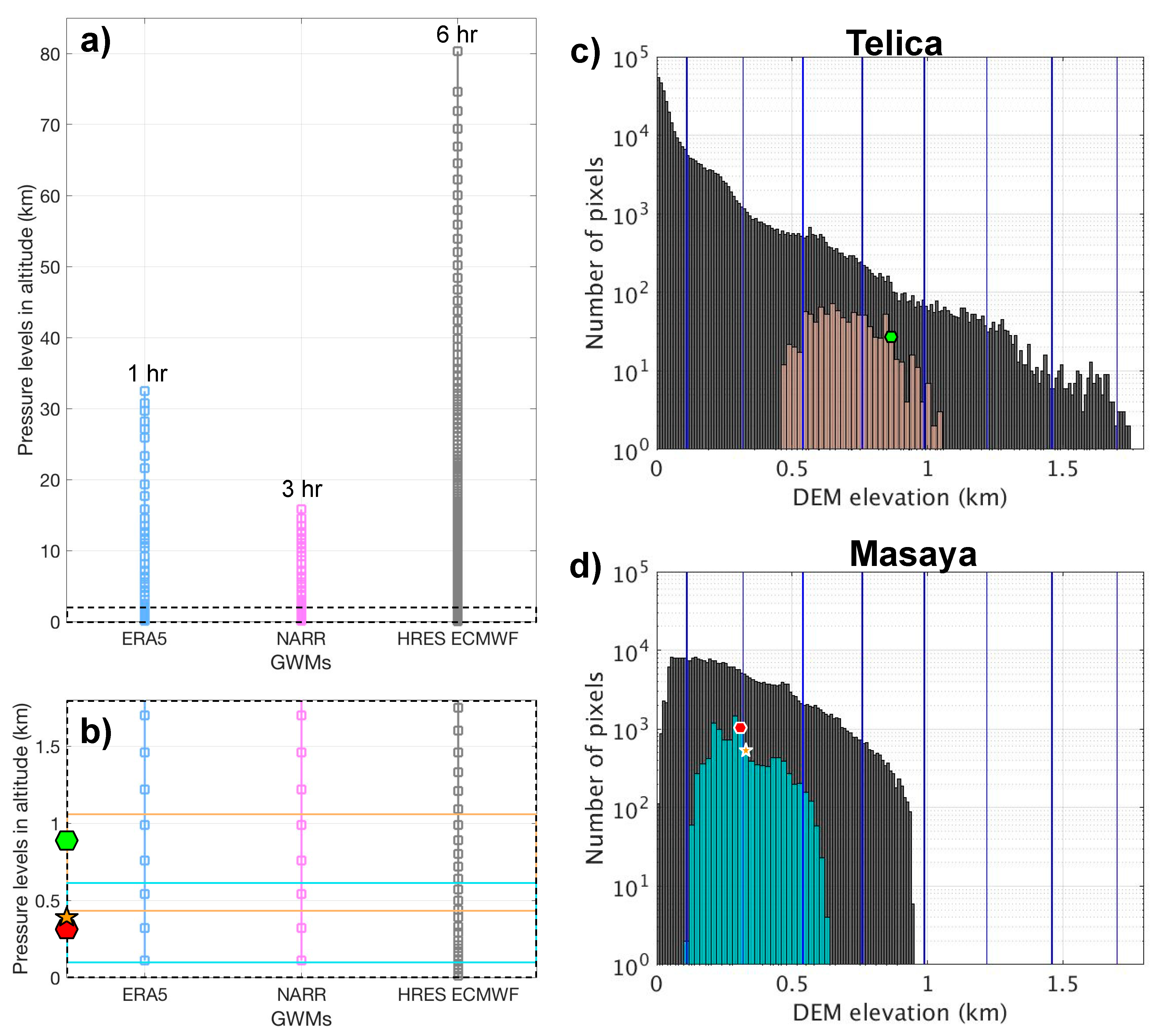
2.3. Global Weather Models (GWMs)
2.4. Statistical Assessments
3. Case Studies
3.1. Telica Volcano
3.1.1. Background
3.1.2. Telica InSAR Dataset
3.1.3. Tropospheric Phase Delay Correction Results
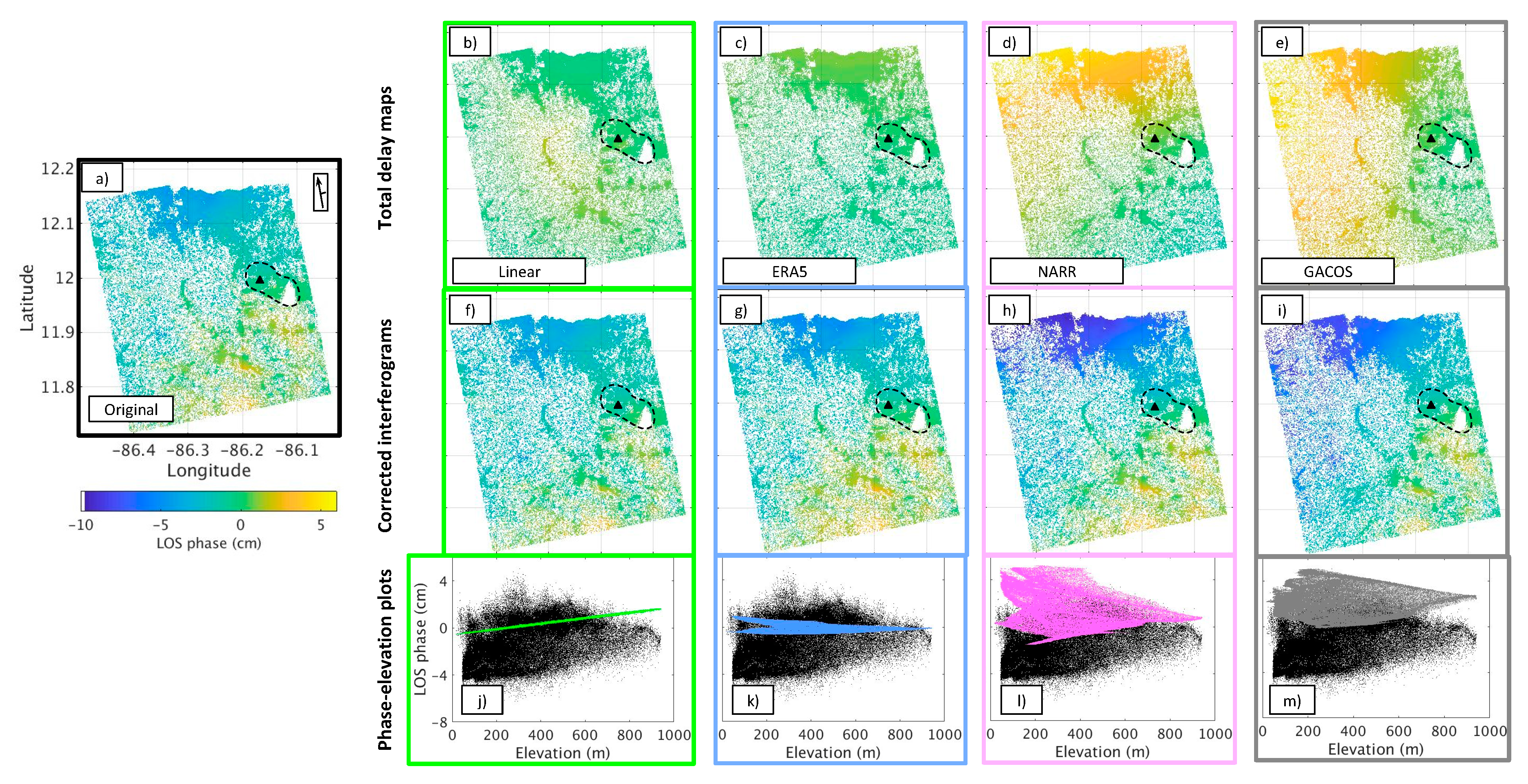
Phase-Elevation Plots
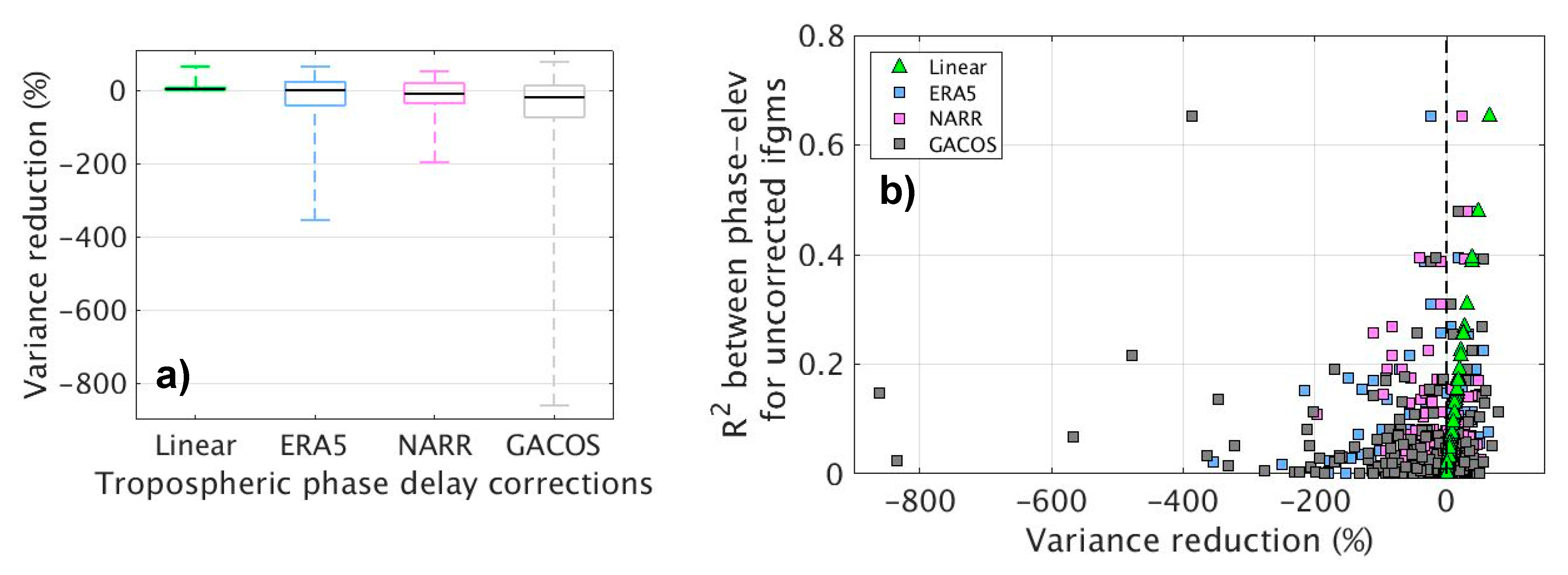
Variance and Variance Reduction
Correcting for Stratified and Turbulent Components
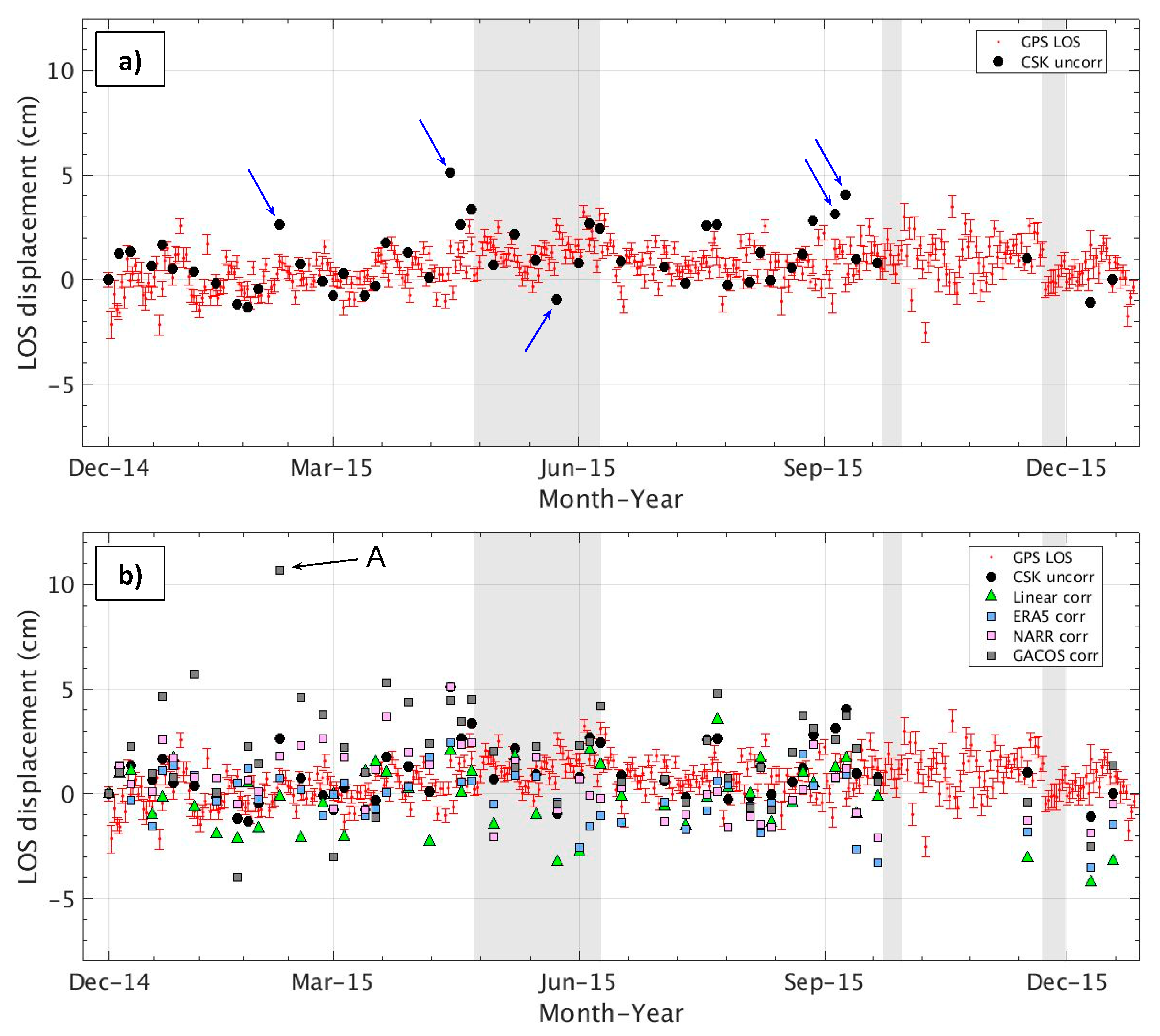
3.1.4. Time-Series Analysis
3.2. Masaya Volcano
3.2.1. Background
3.2.2. Masaya InSAR Dataset
3.2.3. Tropospheric Phase Delay Correction Results
Phase-Elevation Plots
Variance and Variance Reduction
Correcting for Stratified and Turbulent Components
3.2.4. Time-Series Analysis
4. Discussion
4.1. Statistical Assessments Results
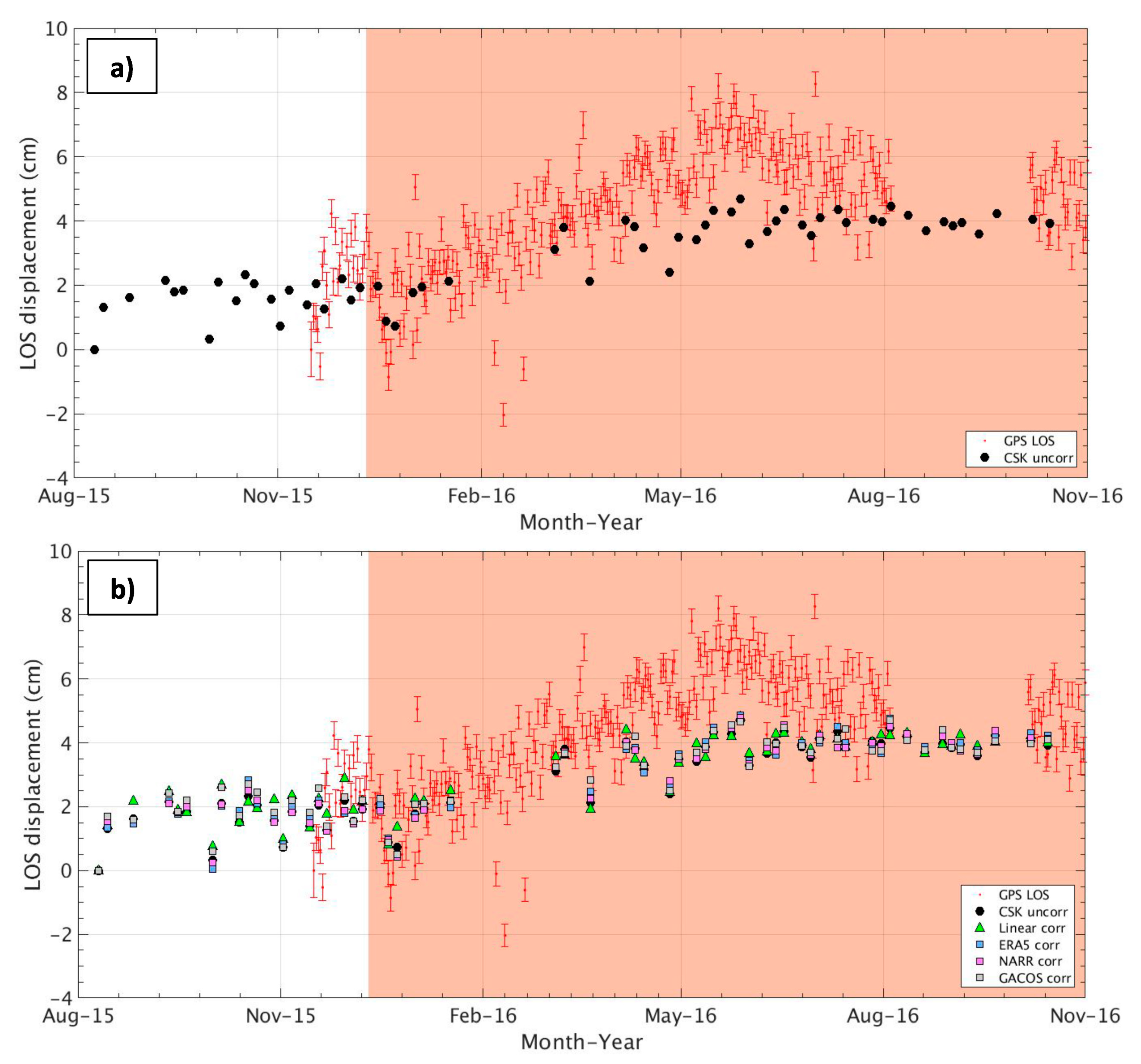
4.2. Time-Series Results (InSAR and GPS)
4.2.1. Telica GPS Results
4.2.2. Masaya GPS Results
4.3. Comparison of Tropospheric Phase Delay Corrections
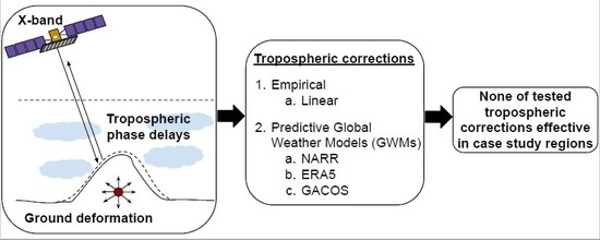
5. Conclusions
Supplementary Materials
Author Contributions
Funding
Acknowledgments
Conflicts of Interest
Abbreviations
| CAVA | Central American Volcanic Arc |
| CSK | COSMO-SkyMed |
| ECMWF | European Center for Medium-Range Weather Forecasts |
| ERA-I | ERA-Interim |
| GACOS | Generic Atmospheric Corrections Online Service for InSAR |
| GPS | Global Positioning System |
| GWM | Global Weather Model |
| HRES ECMWF | High-RESolution European Center for Medium-Range Weather Forecasts |
| INETER | Instituto Nicaragüense de Estudios Territoriales |
| InSAR | Interferometric Synthetic Aperture Radar |
| LOS | Line-Of-Sight |
| MERRA | Modern-Era Retrospective Analysis for Research and Applications |
| MODIS | Moderate Resolution Imaging Spectroradiometer |
| NARR | North American Regional Reanalysis |
| NCEP-NCAR | National Centers for Environmental Prediction- National Center for Atmospheric Research |
| SAR | Synthetic Aperture Radar |
| SBAS | Small BAseline Subset |
| UTC | Coordinated Universal Time |
References
- Burgmann, R.; Rosen, P.A.; Fielding, E.J. Synthetic Aperture Radar Interferometry to Measure Earth’s Surface Topography and Its Deformation. Annu. Rev. Earth Planet. Sci. 2000, 28, 169–209. [Google Scholar] [CrossRef]
- Pinel, V.; Poland, M.P.; Hooper, A. Volcanology: Lessons Learned from Synthetic Aperture Radar Imagery. J. Volcanol. Geotherm. Res. 2014, 289, 81–113. [Google Scholar] [CrossRef]
- Fernández, J.; Pepe, A.; Poland, M.P.; Sigmundsson, F. Volcano Geodesy: Recent Developments and Future Challenges. J. Volcanol. Geotherm. Res. 2017, 344, 1–12. [Google Scholar] [CrossRef]
- Ebmeier, S.K.; Andrews, B.J.; Araya, M.C.; Arnold, D.W.D.; Biggs, J.; Cooper, C.; Cottrell, E.; Furtney, M.; Hickey, J.; Jay, J.; et al. Synthesis of Global Satellite Observations of Magmatic and Volcanic Deformation: Implications for Volcano Monitoring & the Lateral Extent of Magmatic Domains. J. Appl. Volcanol. 2018, 7, 26. [Google Scholar] [CrossRef]
- Stephens, K.J.; Wauthier, C. Satellite Geodesy Captures Offset Magma Supply Associated with Lava Lake Appearance at Masaya Volcano, Nicaragua. Geophys. Res. Lett. 2018, 45, 2669–2678. [Google Scholar] [CrossRef]
- Neal, C.A.; Brantley, S.R.; Antolik, L.; Babb, J.L.; Burgess, M.; Calles, K.; Cappos, M.; Chang, J.C.; Conway, S.; Desmither, L.; et al. The 2018 Rift Eruption and Summit Collapse of Kilauea Volcano. Science 2019, 363, 367–374. [Google Scholar] [CrossRef]
- Smets, B.; Wauthier, C.; D’Oreye, N. A New Map of the Lava Flow Field of Nyamulagira (D.R. Congo) from Satellite Imagery. J. Afr. Earth Sci. 2010, 58, 778–786. [Google Scholar] [CrossRef]
- Ebmeier, S.K.; Biggs, J.; Mather, T.A.; Elliott, J.R.; Wadge, G.; Amelung, F. Measuring Large Topographic Change with InSAR: Lava Thicknesses, Extrusion Rate and Subsidence Rate at Santiaguito Volcano, Guatemala. Earth Planet. Sci. Lett. 2012, 335, 216–225. [Google Scholar] [CrossRef] [Green Version]
- Montgomery-Brown, E.K.; Poland, M.P.; Miklius, A. Delicate Balance of Magmatic-tectonic Interaction at Kilauea Volcano, Hawaii, Revealed from Slow Slip Events. In Hawaiian Volcanoes: From Source to Surface, Geophysical Monograph 208; Carey, R., Cayol, V., Poland, M.P., Weis, D., Eds.; John Wiley & Sons, Inc.: Hoboken, NJ, USA, 2015; pp. 269–288. [Google Scholar] [CrossRef]
- Schaefer, L.N.; Wang, T.; Escobar-Wolf, R.; Oommen, T.; Lu, Z.; Kim, J.; Lundgren, P.R.; Waite, G.P. Three-Dimensional Displacements of a Large Volcano Flank Movement during the May 2010 Eruptions at Pacaya Volcano, Guatemala. Geophys. Res. Lett. 2017, 44, 135–142. [Google Scholar] [CrossRef] [Green Version]
- Arnold, D.W.D.; Biggs, J.; Dietterich, H.R.; Vallejo Vargas, S.; Wadge, G.; Mothes, P. Lava Flow Morphology at an Erupting Andesitic Stratovolcano: A Satellite Perspective on El Reventador, Ecuador. J. Volcanol. Geotherm. Res. 2019, 372, 34–47. [Google Scholar] [CrossRef]
- Hanssen, R.F. Radar Interferometry—Data Interpretation and Error Analysis; Kluwer Academic Publishers: Dordrecht, The Netherlands, 2001. [Google Scholar]
- Massonnet, D.; Feigl, K.L. Radar Interferometry and Its Application to Changes in the Earth’s Surface. Rev. Geophys. 1998, 36, 441. [Google Scholar] [CrossRef] [Green Version]
- Zebker, H.A.; Villasenor, J. Decorrelation in Interferometric Radar Echoes. IEEE Trans. Geosci. Remote Sens. 1992, 30, 950–959. [Google Scholar] [CrossRef] [Green Version]
- Simons, M.; Rosen, P.A. Interferometric Synthetic Aperture Radar Geodesy. In Treatise on Geophysics; Schubert, G., Ed.; Elsevier: Oxford, UK, 2015; Volume 3, pp. 339–385. [Google Scholar] [CrossRef]
- Böhm, J.; Schuh, H. (Eds.) Atmospheric Effects in Space Geodesy; Springer: Berlin/Heidelberg, Germany, 2013. [Google Scholar] [CrossRef]
- Gray, A.L.; Mattar, K.E.; Sofko, G. Influence of Ionospheric Electron Density Fluctuations on Satellite Radar Interferometry. Geophys. Res. Lett. 2000, 27, 1451–1454. [Google Scholar] [CrossRef]
- Fattahi, H.; Simons, M.; Agram, P. InSAR Time-Series Estimation of the Ionospheric Phase Delay: An Extension of the Split Range-Spectrum Technique. IEEE Trans. Geosci. Remote Sens. 2017, 55, 5984–5996. [Google Scholar] [CrossRef]
- Delacourt, C.; Briole, P.; Achache, J. Tropospheric Corrections of SAR Interferograms with Strong Topography. Application to Etna. Geophys. Res. Lett. 1998, 25, 2849–2852. [Google Scholar] [CrossRef]
- Zebker, H.A.; Rosen, P.A.; Hensley, S. Atmospheric Effects in Interferometric Synthetic Aperture Radar Surface Deformation and Topographic Maps. J. Geophys. Res. 1997, 102, 7547–7563. [Google Scholar] [CrossRef]
- Dong, J.; Zhang, L.; Liao, M.; Gong, J. Improved Correction of Seasonal Tropospheric Delay in InSAR Observations for Landslide Deformation Monitoring. Remote Sens. Environ. 2019, 233, 111370. [Google Scholar] [CrossRef]
- Danklmayer, A.; Chandra, M. Precipitation Induced Signatures in SAR Images. In Proceedings of the 3rd European Conference on Antennas and Propagation, EuCAP 2009, Berlin, Germany, 23–27 March 2009; IEEE: Berlin, Germany, 2009; pp. 3433–3437. [Google Scholar]
- Beauducel, F.; Briole, P.; Froger, J.-L. Volcano-Wide Fringes in ERS Synthetic Aperture Radar Interferograms of Etna (1992–1998): Deformation or Tropospheric Effect? J. Geophys. Res. 2000, 105, 16391–16402. [Google Scholar] [CrossRef]
- Wicks, C.W., Jr.; Dzurisin, D.; Ingebritsen, S.; Thatcher, W.; Lu, Z.; Iverson, J. Magmatic Activity beneath the Quiescent Three Sisters Volcanic Center, Central Oregon Cascade Range, USA. Geophys. Res. Lett. 2002, 29, 26-1–26-4. [Google Scholar] [CrossRef] [Green Version]
- Cavalié, O.; Doin, M.P.; Lasserre, C.; Briole, P. Ground Motion Measurement in the Lake Mead Area, Nevada, by Differential Synthetic Aperture Radar Interferometry Time Series Analysis: Probing the Lithosphere Rheological Structure. J. Geophys. Res. 2007, 112. [Google Scholar] [CrossRef] [Green Version]
- Lin, Y.N.N.; Simons, M.; Hetland, E.A.; Muse, P.; DiCaprio, C. A Multiscale Approach to Estimating Topographically Correlated Propagation Delays in Radar Interferograms. Geochem. Geophys. Geosyst. 2010, 11. [Google Scholar] [CrossRef]
- Bekaert, D.P.S.; Walters, R.J.; Wright, T.J.; Hooper, A.J.; Parker, D.J. Statistical Comparison of InSAR Tropospheric Correction Techniques. Remote Sens. Environ. 2015, 170, 40–47. [Google Scholar] [CrossRef] [Green Version]
- Bekaert, D.P.S.; Hooper, A.J.; Wright, T.J. A Spatially Variable Power Law Tropospheric Correction Technique for InSAR Data. J. Geophys. Res. 2015, 120, 1345–1356. [Google Scholar] [CrossRef]
- Murray, K.D.; Bekaert, D.P.S.; Lohman, R.B. Tropospheric Corrections for InSAR: Statistical Assessments and Applications to the Central United States and Mexico. Remote Sens. Environ. 2019, 232, 111326. [Google Scholar] [CrossRef]
- Bevis, M.; Businger, S.; Herring, T.A.; Rocken, C.; Anthes, R.A.; Ware, R.H. GPS Meteorology: Remote Sensing of Atmospheric Water Vapor Using the Global Positioning System. J. Geophys. Res. 1992, 97, 15787–15801. [Google Scholar] [CrossRef]
- Doin, M.-P.; Lasserre, C.; Peltzer, G.; Cavalié, O.; Doubre, C. Corrections of Stratified Tropospheric Delays in SAR Interferometry: Validation with Global Atmospheric Models. J. Appl. Geophys. 2009, 69, 35–50. [Google Scholar] [CrossRef]
- Jolivet, R.; Grandin, R.; Lasserre, C.; Doin, M.-P.; Peltzer, G. Systematic InSAR Tropospheric Phase Delay Corrections from Global Metereological Reanalysis Data. Geophys. Res. Lett. 2011, 38. [Google Scholar] [CrossRef] [Green Version]
- Jolivet, R.; Agram, P.S.; Lin, N.Y.; Simons, M.; Doin, M.-P.; Peltzer, G.; Li, Z. Improving InSAR Geodesy Using Global Atmospheric Models. J. Geophys. Res. Solid Earth 2014, 119, 2324–2341. [Google Scholar] [CrossRef]
- Parker, A.L.; Biggs, J.; Walters, R.J.; Ebmeier, S.K.; Wright, T.J.; Teanby, N.A.; Lu, Z. Systematic Assessment of Atmospheric Uncertainties for InSAR Data at Volcanic Arcs Using Large-Scale Atmospheric Models: Application to the Cascade Volcanoes, United States. Remote Sens. Environ. 2015, 170, 102–114. [Google Scholar] [CrossRef] [Green Version]
- Stephens, K.J.; Ebmeier, S.K.; Young, N.K.; Biggs, J. Transient Deformation Associated with Explosive Eruption Measured at Masaya Volcano (Nicaragua) Using Interferometric Synthetic Aperture Radar. J. Volcanol. Geotherm. Res. 2017, 344, 212–223. [Google Scholar] [CrossRef]
- Cong, X.; Balss, U.; Gonzalez, F.R.; Eineder, M. Mitigation of Tropospheric Delay in SAR and InSAR Using NWP Data: Its Validation and Application Examples. Remote Sens. 2018, 10, 1515. [Google Scholar] [CrossRef] [Green Version]
- Samsonov, S.V.; Trishchenko, A.P.; Tiampo, K.; González, P.J.; Zhang, Y.; Fernández, J. Removal of Systematic Seasonal Atmospheric Signal from Interferometric Synthetic Aperture Radar Ground Deformation Time Series. Geophys. Res. Lett. 2014, 41, 6123–6130. [Google Scholar] [CrossRef] [Green Version]
- Heleno, S.I.N.; Frischknecht, C.; D’Oreye, N.; Lima, J.N.P.; Faria, B.; Wall, R.; Kervyn, F. Seasonal Tropospheric Influence on SAR Interferograms near the ITCZ—The Case of Fogo Volcano and Mount Cameroon. J. Afr. Earth Sci. 2010, 58, 833–856. [Google Scholar] [CrossRef] [Green Version]
- Li, Z.; Fielding, E.J.; Cross, P.; Preusker, R. Advanced InSAR Atmospheric Correction: MERIS/MODIS Combination and Stacked Water Vapour Models. Int. J. Remote Sens. 2009, 30, 3343–3363. [Google Scholar] [CrossRef]
- Wadge, G.; Webley, P.W.; James, I.N.; Bingley, R.; Dodson, A.; Waugh, S.; Veneboer, T.; Puglisi, G.; Mattia, M.; Baker, D.; et al. Atmospheric Models, GPS and InSAR Measreuments of the Tropospheric Water Vapour Field over Mount Etna. Geophys. Res. Lett. 2002, 29, 11-1–11-4. [Google Scholar] [CrossRef] [Green Version]
- Webley, P.W.; Wadge, G.; James, I.N. Determining Radio Wave Delay by Non-Hydrostatic Atmospheric Modelling of Water Vapour over Mountains. Phys. Chem. Earth 2004, 29, 139–148. [Google Scholar] [CrossRef]
- Foster, J.; Brooks, B.; Cherubini, T.; Shacat, C.; Businger, S.; Werner, C.L. Mitigating Atmospheric Noise for InSAR Using a High Resolution Weather Model. Geophys. Res. Lett. 2006, 33. [Google Scholar] [CrossRef]
- Li, Z.; Muller, J.-P.; Cross, P.; Fielding, E.J. Interferometric Synthetic Aperture Radar (InSAR) Atmospheric Correction: GPS, Moderate Resolution Imaging Spectrometer (MODIS), and InSAR Integration. J. Geophys. Res. 2005, 110. [Google Scholar] [CrossRef]
- Yu, C.; Li, Z.; Penna, N.T.; Crippa, P. Generic Atmospheric Correction Model for Interferometric Synthetic Aperture Radar Observations. J. Geophys. Res. Solid Earth 2018, 12, 9202–9222. [Google Scholar] [CrossRef]
- Pinel, V.; Hooper, A.; De la Cruz-Reyna, S.; Reyes-Davila, G.; Doin, M.P.; Bascou, P. The Challenging Retrieval of the Displacement Field from InSAR Data for Andesitic Stratovolcanoes: Case Study of Popocatepetl and Colima Volcano, Mexico. J. Volcanol. Geotherm. Res. 2011, 200, 49–61. [Google Scholar] [CrossRef]
- Welch, M.D.; Schmidt, D.A. Separating Volcanic Deformation and Atmospheric Signals at Mount St. Helens Using Persistent Scatterer InSAR. J. Volcanol. Geotherm. Res. 2017, 344, 52–64. [Google Scholar] [CrossRef]
- Neelmeijer, J.; Schöne, T.; Dill, R.; Klemann, V.; Motagh, M. Ground Deformations around the Toktogul Reservoir, Kyrgyzstan, from Envisat ASAR and Sentinel-1 Data—A Case Study about the Impact of Atmospheric Corrections on InSAR Time Series. Remote Sens. 2018, 10, 462. [Google Scholar] [CrossRef] [Green Version]
- Hu, Z.; Mallorquí, J.J. An Accurate Method to Correct Atmospheric Phase Delay for InSAR with the ERA5 Global Atmospheric Model. Remote Sens. 2019, 11, 1969. [Google Scholar] [CrossRef] [Green Version]
- Albino, F.; Biggs, J.; Syahbana, D.K. Dyke Intrusion between Neighbouring Arc Volcanoes Responsible for 2017 Pre-Eruptive Seismic Swarm at Agung. Nat. Commun. 2019, 10. [Google Scholar] [CrossRef] [PubMed] [Green Version]
- Guo, Q.; Xu, C.; Wen, Y.; Liu, Y.; Xu, G. The 2017 Noneruptive Unrest at the Caldera of Cerro Azul Volcano (Galápagos Islands) Revealed by InSAR Observations and Geodetic Modelling. Remote Sens. 2019, 11, 1992. [Google Scholar] [CrossRef] [Green Version]
- Wang, X.; Aoki, Y. Posteruptive Thermoelastic Deflation of Intruded Magma in Usu Volcano, Japan, 1992–2017. J. Geophys. Res. Solid Earth 2019, 124, 335–357. [Google Scholar] [CrossRef]
- Wang, Q.; Yu, W.; Xu, B.; Wei, G. Assessing the Use of GACOS Products for SBAS-InSAR Deformation Monitoring: A Case in Southern California. Sensors 2019, 19, 3894. [Google Scholar] [CrossRef]
- Yip, S.T.H.; Biggs, J.; Albino, F. Reevaluating Volcanic Deformation Using Atmospheric Corrections: Implications for the Magmatic System of Agung Volcano, Indonesia. Geophys. Res. Lett. 2019, 46, 1–8. [Google Scholar] [CrossRef] [Green Version]
- Albino, F.; Biggs, J.; Yu, C.; Li, Z. Automated Methods for Detecting Volcanic Deformation Using Sentinel-1 InSAR Time Series Illustrated by the 2017–2018 Unrest at Agung, Indonesia. J. Geophys. Res. Solid Earth 2020. [Google Scholar] [CrossRef] [Green Version]
- Lundgren, P.; Usai, S.; Sansosti, E.; Lanari, R.; Tesauro, M.; Fornaro, G.; Berardino, P. Modeling Surface Deformation Observed with Synthetic Aperture Radar Interferometry at Campi Flegrei Caldera. J. Geophys. Res. 2001, 106, 19355–19366. [Google Scholar] [CrossRef] [Green Version]
- Berardino, P.; Fornaro, G.; Lanari, R.; Sansosti, E. A New Algorithm for Surface Deformation Monitoring Based on Small Baseline Differential SAR Interferograms. IEEE Trans. Geosci. Remote Sens. 2002, 40, 2375–2383. [Google Scholar] [CrossRef] [Green Version]
- Werner, C.; Wegmüller, U.; Strozzi, T.; Wiesmann, A. GAMMA SAR and Interferometric Processing Software. ERS-ENVISAT Symposium, Gothenburg, Sweden. 2000. Available online: http://citeseerx.ist.psu.edu/viewdoc/download?doi=10.1.1.20.6363&rep=rep1&type=pdf (accessed on 1 March 2020).
- Rizzoli, P.; Martone, M.; Gonzalez, C.; Wecklich, C.; Borla Tridon, D.; Bräutigam, B.; Bachmann, M.; Schulze, D.; Fritz, T.; Huber, M.; et al. Generation and Performance Assessment of the Global TanDEM-X Digital Elevation Model. ISPRS J. Photogramm. Remote Sens. 2017, 132, 119–139. [Google Scholar] [CrossRef] [Green Version]
- Wessel, B.; Huber, M.; Wolfhart, C.; Marschalk, U.; Kosmann, D.; Roth, A. Accuracy Assessment of the Global TanDEM-X Digital Elevation Model with GPS Data. ISPRS J. Photogramm. Remote Sens. 2018, 139, 171–182. [Google Scholar] [CrossRef]
- Goldstein, R.M.; Werner, C.L. Radar Interferogram Filtering for Geophysical Applications. Geophys. Res. Lett. 1998, 25, 4035–4038. [Google Scholar] [CrossRef] [Green Version]
- Costantini, M. A Novel Phase Unwrapping Method Based on Network Programming. IEEE Trans. Geosci. Remote Sens. 1998, 36, 813–821. [Google Scholar] [CrossRef]
- Zumberge, J.F.; Heflin, M.B.; Jefferson, D.C.; Watkins, M.M.; Webb, F.H. Precise Point Positioning for the Efficient and Robust Analysis of GPS Data from Large Networks. J. Geophys. Res. 1997, 102, 5005–5017. [Google Scholar] [CrossRef] [Green Version]
- Bertiger, W.; Desai, S.D.; Haines, B.; Harvey, N.; Moore, A.W.; Owen, S.; Weiss, J.P. Single Receiver Phase Ambiguity Resolution with GPS Data. J. Geod. 2010, 84, 327–337. [Google Scholar] [CrossRef]
- Lyard, F.; Lefevre, F.; Letellier, T.; Francis, O. Modelling the Global Ocean Tides: Modern Insights from FES2004. Ocean Dyn. 2006, 56, 394–415. [Google Scholar] [CrossRef]
- Boehm, J.; Werl, B.; Schuh, H. Troposphere Mapping Functions for GPS and Very Long Baseline Interferometry from European Centre for Medium-Range Weather Forecasts Operational Analysis Data. J. Geophys. Res. 2006, 111, B02406. [Google Scholar] [CrossRef]
- Rebischung, P.; Griffiths, J.; Ray, J.; Schmid, R.; Collilieux, X.; Garayt, B. IGS08: The IGS Realization of ITRF2008. GPS Solut. 2012, 16, 483–494. [Google Scholar] [CrossRef]
- Fialko, Y.; Simons, M.; Agnew, D. The Complete (3-D) Surface Displacement Field in the Epicentral Area of the 1999 Mw 7.1 Hector Mine Earthquake, California from Space Geodetic Observations. Geophys. Res. Lett. 2001, 28, 3063–3066. [Google Scholar] [CrossRef] [Green Version]
- Mesinger, F.; DiMego, G.; Kalnay, E.; Mitchell, K.; Shafran, P.C.; Ebisuzaki, W.; Jović, D.; Woollen, J.; Rogers, E.; Berbery, E.H.; et al. North American Regional Reanalysis. Bull. Am. Meteorol. Soc. 2006, 87, 343–360. [Google Scholar] [CrossRef] [Green Version]
- Rogers, E.; Lin, Y.; Mitchell, K.; Wu, W.-S.; Ferrier, B.; Gayno, G.; Pondeca, M.; Pyle, M.; Wong, V.; Ek, M. The NCEP North American Modeling System: Final Eta Model Analysis Changes and Preliminary Experiments Using the WRF-NMM. In Proceedings of the 21st Conference on Weather Analysis and Forecasting/17th Conference on Numerical Weather Prediction; American Meteorological Society; Washington, DC, USA, 2005. [Google Scholar]
- Copernicus Climate Change Service (C3S). ERA5: Fifth Generation of ECMWF Atmospheric Reanalysis of the Global Climate. 2017. Available online: https://cds.climate.copernicus.eu/cdsapp#!/home (accessed on 1 March 2020).
- Hersbach, H.; De Rosnay, P.; Bell, B.; Schepers, D.; Simmons, A.; Soci, C.; Abdalla, S.; Balmaseda, A.; Balsamo, G.; Bechtold, P.; et al. Operational Global Reanalysis: Progress, Future Directions and Synergies with NWP Including Updates on the ERA5 Production Status. ERA Rep. Ser. 2018. [Google Scholar] [CrossRef]
- Baby, H.B.; Gole, P.; Lavergnat, J. A Model for the Tropospheric Excess Path Length of Radio Waves from Surface Meteorological Measurements. Radio Sci. 1988, 23, 1023–1038. [Google Scholar] [CrossRef]
- Smith, E.K.; Weintraub, S. The Constants in the Equation for Atmospheric Refractive Index at Radio Frequencies. Proc. IRE 1952, 41, 1035–1037. [Google Scholar] [CrossRef] [Green Version]
- Yu, C.; Penna, N.T.; Li, Z. Generation of Real-Time Mode High-Resolution Water Vapor Fields from GPS Observations. J. Geophys. Res. Atmos. 2017, 122, 2008–2025. [Google Scholar] [CrossRef]
- Yu, C.; Li, Z.; Penna, N.T. Interferometric Synthetic Aperture Radar Atmospheric Correction Using a GPS-Based Iterative Tropospheric Decomposition Model. Remote Sens. Environ. 2018, 204, 109–121. [Google Scholar] [CrossRef]
- Ebmeier, S.K.; Biggs, J.; Mather, T.A.; Amelung, F. On the Lack of InSAR Observations of Magmatic Deformation at Central American Volcanoes. J. Geophys. Res. Solid Earth 2013, 118, 2571–2585. [Google Scholar] [CrossRef]
- Ebmeier, S.K.; Biggs, J.; Mather, T.A.; Amelung, F. Applicability of InSAR to Tropical Volcanoes: Insights from Central America. Geol. Soc. Lond. Spec. Publ. 2013, 380, 15–37. [Google Scholar] [CrossRef] [Green Version]
- Peel, M.C.; Finlayson, B.L.; McMahon, T.A. Updated World Map of the Köppen–Geiger Climate Classification. Hydrol. Earth Syst. Sci. 2007, 11, 1633–1644. [Google Scholar] [CrossRef] [Green Version]
- Global Volcanism Program. Telica (344040). Volcanoes of the World. 2013. Available online: https://volcano.si.edu/volcano.cfm?vn=344040 (accessed on 1 March 2020).
- Geirsson, H.; Rodgers, M.; LaFemina, P.; Witter, M.; Roman, D.; Muñoz, A.; Tenorio, V.; Alvarez, J.; Jacobo, V.C.; Nilsson, D.; et al. Multidisciplinary Observations of the 2011 Explosive Eruption of Telica Volcano, Nicaragua: Implications for the Dynamics of Low-Explosivity Ash Eruptions. J. Volcanol. Geotherm. Res. 2014, 271, 55–69. [Google Scholar] [CrossRef]
- Roman, D.C.; LaFemina, P.C.; Bussard, R.; Stephens, K.J.; Wauthier, C.; Higgins, M.; Feineman, M.; Arellano, S.; de Moor, J.M.; Avard, G.; et al. Mechanisms of Unrest and Eruption at Persistently Restless Volcanoes: Insights from the 2015 Eruption of Telica Volcano, Nicaragua. Geochem. Geophys. Geosyst. 2019, 20, 4162–4183. [Google Scholar] [CrossRef] [Green Version]
- Global Volcanism Program. Volcanoes of the World. v. 4.8.0. 2013. Available online: https://doi.org/10.5479/si.GVP.VOTW4-2013 (accessed on 1 March 2020).
- World Population Review. Population of Cities in Nicaragua. 2019. Available online: http://worldpopulationreview.com/countries/nicaragua-population/cities/ (accessed on 25 August 2019).
- Global Volcanism Program. Masaya (344100). Volcanoes of the World. 2013. Available online: https://volcano.si.edu/volcano.cfm?vn=344100 (accessed on 1 March 2020). [CrossRef]
- McBirney, A.R. The Nicaraguan Volcano Masaya and Its Caldera. EOS Trans. Am. Geophys. Union 1956, 37, 83–96. [Google Scholar] [CrossRef]
- Bice, D. Tephra Stratigraphy and Physical Aspects of Recent Volcanism near Managua, Nicaragua. Ph.D. Thesis, University of California, Berkeley, CA, USA, 1980. [Google Scholar]
- Kutterolf, S.; Freundt, A.; Pérez, W.; Wehrmann, H.; Schmincke, H.U. Late Pleistocene to Holocene Temporal Succession and Magnitudes of Highly-Explosive Volcanic Eruptions in West-Central Nicaragua. J. Volcanol. Geotherm. Res. 2007, 163, 55–82. [Google Scholar] [CrossRef]
- Rymer, H.; van Wyk de Vries, B.; Stix, J.; Williams-Jones, G. Pit Crater Structure and Processes Governing Persistent Activity at Masaya Volcano, Nicaragua. Bull. Volcanol. 1998, 59, 345–355. [Google Scholar] [CrossRef]
- Stoiber, R.E.; Williams, S.N.; Huebert, B.J. Sulfur and Halogen Gases at Masaya Caldera Complex, Nicaragua: Total Flux and Variaations with Time. J. Geophys. Res. 1986, 91, 12215–12231. [Google Scholar] [CrossRef]
- INETER. Boletín Mensual Sismos y Volcanes de Nicaragua, Diciembre 2015. 2015. Available online: http://webserver2.ineter.gob.ni/boletin/2015/12/index1512.htm (accessed on 1 March 2020).
- INETER. Boletín Mensual: Sismos y Volcanes de Nicaragua, Octubre 2006. 2006. Available online: https://webserver2.ineter.gob.ni//boletin/2006/10/volcan-masaya0610.htm (accessed on 1 March 2020).
- Murray, J.; Caravantes Gonzalez, G.; Rymer, H.; Williams-Jones, G.; Ferrucci, F. Recent Inflation at Masay Volcano, Nicaragua. In IAVCEI 2017 Scientific Assembly: Fostering Integrative Studies of Volcanoes; IAVCEI: Portland, OR, USA, 2017; p. 739. [Google Scholar]
- Rymer, H.; Williams-Jones, G.; Murray, J.; Delmelle, P.; Reid, K.; Caravantes Gonzalez, G. Precursors to the Current Activity at Masaya Volcano, Nicaragua. In IAVCEI 2017 Scientific Assembly: Fostering Integrative Studies of Volcanoes; IAVCEI: Portland, OR, USA, 2017; p. 939. [Google Scholar]
- Aiuppa, A.; de Moor, J.M.; Arellano, S.; Coppola, D.; Francofonte, V.; Galle, B.; Giudice, G.; Liuzzo, M.; Mendoza, E.; Saballos, A.; et al. Tracking Formation of a Lava Lake from Ground and Space: Masaya Volcano (Nicaragua), 2014–2017. Geochem. Geophys. Geosyst. 2018, 19, 496–515. [Google Scholar] [CrossRef]
- De Moor, J.M.; Kern, C.; Avard, G.; Muller, C.; Aiuppa, A.; Saballos, A.; Ibarra, M.; LaFemina, P.; Protti, M.; Fischer, T.P. A New Sulfur and Carbon Degassing Inventory for the Southern Central American Volcanic Arc: The Importance of Accurate Time-Series Datasets and Possible Tectonic Processes Responsible for Temporal Variations in Arc-Scale Volatile Emissions. Geochem. Geophys. Geosyst. 2017, 18, 4437–4468. [Google Scholar] [CrossRef]
- Emardson, T.R.; Simons, M.; Webb, F.H. Neutral Atmospheric Delay in Interferometric Synthetic Aperture Radar Applications: Statistical Description and Mitigation. J. Geophys. Res. 2003, 108. [Google Scholar] [CrossRef]
- Jolivet, R.; Lasserre, C.; Doin, M.P.; Guillaso, S.; Peltzer, G.; Dailu, R.; Sun, J.; Shen, Z.K.; Xu, X. Shallow Creep on the Haiyuan Fault (Gansu, China) Revealed by SAR Interferometry. J. Geophys. Res. 2012, 117. [Google Scholar] [CrossRef] [Green Version]
- Wessel, P.; Smith, W.H.F. New, Improved Version of the Generic Mapping Tools Released. EOS Trans. Am. Geophys. Union 1998, 79, 579. [Google Scholar] [CrossRef]


| GWMs | Spatial Resolution | Temporal Resolution | Vertical Resolution |
|---|---|---|---|
| NARR | 0.3° × 0.3° (32 km) | 3 h (00, 03, 06, 09, 12, 15, 18, 21) | 29 levels (1000–100 hPa) |
| ERA5 | 0.281° × 0.281° (30 km) | Hourly | 37 levels (1000–1 hPa) |
| HRES ECMWF (GACOS) | 0.125° × 0.125° (14 km) | 6 h (00, 06, 12, 18) | 137 levels (1000–0.01 hPa) |
| Variable | Values |
|---|---|
| k1 | 0.776 K.Pa−1 |
| k2 | 0.716 K.Pa−1 |
| k3 | 3750 K2.Pa−1 |
| Rd | 287.05 J.kg−1.K−1 |
| Rv | 461.495 J.kg−1.K−1 |
| Correction Method | Telica | Masaya | ||
|---|---|---|---|---|
| Var (cm2) | Var Red (%) | Var (cm2) | Var Red (%) | |
| Uncorrected | 5.44 (0.60, 43.94) | – | 5.69 (0.71, 47.55) | – |
| Linear | 5.23 (0.55, 43.51) | 5.97 (–0.33, 65.40) | 5.43 (0.49, 47.44) | 6.65 (–3.21, 42.47) |
| ERA5 | 5.55 (0.65, 44.21) | –17.58 (–353.73, 64.19) | 6.36 (4.46, 64.40) | –20.94 (–675.48, 70.12) |
| NARR | 5.54 (0.79, 46.32) | −11.63 (–197.08, 51.80) | 6.68 (0.56, 62.82) | –24.56 (–364.80, 58.07) |
| GACOS | 6.58 (0.74, 54.89) | –53.61 (–863.31, 78.30) | 5.92 (0.64, 50.90) | –20.37 (–286.53, 83.32) |
© 2020 by the authors. Licensee MDPI, Basel, Switzerland. This article is an open access article distributed under the terms and conditions of the Creative Commons Attribution (CC BY) license (http://creativecommons.org/licenses/by/4.0/).
Share and Cite
Stephens, K.J.; Wauthier, C.; Bussard, R.C.; Higgins, M.; LaFemina, P.C. Assessment of Mitigation Strategies for Tropospheric Phase Contributions to InSAR Time-Series Datasets over Two Nicaraguan Volcanoes. Remote Sens. 2020, 12, 782. https://doi.org/10.3390/rs12050782
Stephens KJ, Wauthier C, Bussard RC, Higgins M, LaFemina PC. Assessment of Mitigation Strategies for Tropospheric Phase Contributions to InSAR Time-Series Datasets over Two Nicaraguan Volcanoes. Remote Sensing. 2020; 12(5):782. https://doi.org/10.3390/rs12050782
Chicago/Turabian StyleStephens, Kirsten J., Christelle Wauthier, Rebecca C. Bussard, Machel Higgins, and Peter C. LaFemina. 2020. "Assessment of Mitigation Strategies for Tropospheric Phase Contributions to InSAR Time-Series Datasets over Two Nicaraguan Volcanoes" Remote Sensing 12, no. 5: 782. https://doi.org/10.3390/rs12050782