A Monte Carlo-Based Outlier Diagnosis Method for Sensitivity Analysis

Abstract

An iterative outlier elimination procedure based on hypothesis testing, commonly known as Iterative Data Snooping (IDS) among geodesists, is often used for the quality control of modern measurement systems in geodesy and surveying. The test statistic associated with IDS is the extreme normalised least-squares residual. It is well-known in the literature that critical values (quantile values) of such a test statistic cannot be derived from well-known test distributions but must be computed numerically by means of Monte Carlo. This paper provides the first results on the Monte Carlo-based critical value inserted into different scenarios of correlation between outlier statistics. From the Monte Carlo evaluation, we compute the probabilities of correct identification, missed detection, wrong exclusion, over-identifications and statistical overlap associated with IDS in the presence of a single outlier. On the basis of such probability levels, we obtain the Minimal Detectable Bias (MDB) and Minimal Identifiable Bias (MIB) for cases in which IDS is in play. The MDB and MIB are sensitivity indicators for outlier detection and identification, respectively. The results show that there are circumstances in which the larger the Type I decision error (smaller critical value), the higher the rates of outlier detection but the lower the rates of outlier identification. In such a case, the larger the Type I Error, the larger the ratio between the MIB and MDB. We also highlight that an outlier becomes identifiable when the contributions of the measures to the wrong exclusion rate decline simultaneously. In this case, we verify that the effect of the correlation between outlier statistics on the wrong exclusion rate becomes insignificant for a certain outlier magnitude, which increases the probability of identification.

1. Introduction

In recent years, Outlier Detection has been increasingly applied in sensor data processing [1,2,3,4,5,6,7,8,9]. Despite the countless contributions made over the years, there is continuing research on the subject, mainly because there has been an increase in computational power. One can argue that computational complexity is becoming high because of the era of information overload. However, this limitation has been overcome over the years, mainly by the rapid development of computers, which now allow advanced computational techniques to be used efficiently on personal computers or even on handheld computers [10]. Therefore, computational complexity is no longer a bottleneck because we have fast computers and large data storage systems at our disposal [11,12].

Here, we assume that an outlier is a measurement that is so likely to be caused by a blunder that it is better to either not use it or not use it as it is [13]. Failure to identify an outlier can jeopardise the reliability level of a system. Because of its importance, outliers must be appropriately treated to ensure the quality of data analysis.

Two categories of advanced techniques for the treatment of a dataset contaminated by outliers have often been developed and applied in various situations: Robust Adjustment Procedures (see, e.g., [14,15,16,17,18]) and Statistical Hypothesis Testing (see, e.g., [2,12,19,20,21,22,23]). The first one is an estimation technique that is not unduly affected by outliers or other small departures from model assumptions. Classes of this technique include M-estimates (which follow from maximum likelihood considerations), L-Estimates (which are linear combinations of order statistics), and R-Estimates (based on statistical rank tests). Some classes of such robust adjustment methods, as well as their properties, are well known, while other methods are still being researched (see, e.g., $L_1$-norm estimation [24], M-estimation [25,26,27], R-estimation [28,29,30] and those based on meta-heuristics [31]). Besides the undoubted advantages of Robust Estimation, here, we focus on the hypothesis test-based outlier. The following advantages of the outlier test were mentioned by [32]:

• It is an opportunity to investigate the causes of outliers;
• Identified outliers can be remeasured; and
• If the outliers are discarded from the measurements, then standard adjustment software, which operates according to the least-squares criterion, can be used.

In this paper, we consider iterative data snooping (IDS), which is the most common procedure found in the geodetic practice [12,33]. Most conventional geodetic studies have a chapter on IDS (see, e.g., [34,35]). IDS has also become very popular and is routinely used in adjustment computations [36]. It is important to mention that IDS is not restricted to the field of geodetic statistics but is a generally applicable method [22].

IDS is an iterative outlier elimination procedure, which combines estimation, testing and adaptation [37]. Parameter estimation is often conducted in the sense of the least-squares estimation (LSE). Assuming that no outlier exists, the LSE is the best linear unbiased estimator (BLUE) [35]. The LSE has often been used in several remote sensing applications (see, e.g., [38,39,40,41]). However, outliers can inevitably occur in practice and cause the loss of the LSE BLUE-property. Then, hypothesis testing is performed with the aim of identifying any outliers that may be present in the dataset. After its identification, the suspected outlier is then excluded from the dataset as a corrective action (i.e., adaptation), and the LSE is restarted without the rejected measurement. If model redundancy permits, this procedure is repeated until no more (possible) outliers can be identified (see, e.g., [35], p. 135). Although here we restrict ourselves to the case of one outlier at a time, IDS can also be applied to the case of multiple (simultaneous) outliers [42]. For more details about multiple (simultaneous) outliers, refer to [43,44,45].

Of particular importance for quality control purposes are decision probabilities. Probability levels have already been described in the literature for the case in which data snooping is run once (i.e., only one single estimation and testing), as well as for the case in which the outlier is parameterised in the model (see, e.g., [2,19,20,21,23,37,46,47]). For such cases, the probability of correct detection (${\mathcal{P}}_{CD}$) and correct identification (${\mathcal{P}}_{CI}$) and their corresponding Minimal Detectable Bias (MDB) and Minimal Identifiable Bias (MIB) have already been described for data snooping [37,46].

The MDB is defined as the smallest value of an outlier that can be detected given a certain ${\mathcal{P}}_{CD}$. The MDB is an indicator of the sensitivity of data snooping to outlier detection and not to outlier identification. On the other hand, the MIB is defined as the smallest value of an outlier that can be identified given a certain ${\mathcal{P}}_{CI}$; i.e., the MIB is an indicator of the sensitivity of data snooping to outlier identification. It is important to highlight that “outlier detection” only informs us whether or not there might have been at least one outlier. However, the detection does not tell us which measurement is an outlier. The localisation of the outlier is a problem of “outlier identification”. In other words, “outlier identification” implies the execution of a search among the measurements for the most likely outlier.

However, both the MDB and MIB cannot be used as a diagnostic tool when IDS is in play. In this contribution, we highlight the fact that the correct outlier identification for IDS is not only dependent on the correct/missed detection and wrong exclusion but also other decision probabilities.

The evaluation of the probability levels associated with IDS is not a trivial task. When used for data snooping for a single run, the probabilities of IDS are multivariate integrals over complex regions [2,47]. This complexity is due to the fact that IDS is not only based on multiple hypothesis testing but also on multiple rounds of estimation, testing and exclusion. Because an analytical formula is not easy to compute, the Monte Carlo method should be run to obtain the probabilities and the minimal bias (MDB and MIB) indicators for IDS. The Monte Carlo method provides insights into these cases, in which analytical solutions are too complex to fully understand, are doubted for one reason or another or are not available [12]. The Monte Carlo method for quality control purposes has already been applied in geodesy (see, e.g., [2,10,22,23,33,46,48,49,50,51]). For in-depth coverage of Monte Carlo methods, consult, for instance, [52,53,54].

Recent studies by Rofatto et al. [12,55] provide an algorithm based on Monte Carlo to determine the probability levels associated with IDS. In that case, five classes of decisions for IDS are described, namely, the probability of correct identification (${\mathcal{P}}_{CI}$), the probability of missed detection (${\mathcal{P}}_{MD}$), the probability of wrong exclusion (${\mathcal{P}}_{WE}$), the probability of over-identification positive (${\mathcal{P}}_{over+}$), and the probability of over-identification negative (${\mathcal{P}}_{over-}$), defined as follows:

• ${\mathcal{P}}_{CI}$: The probability of correctly identifying and removing an outlying measurement;
• ${\mathcal{P}}_{MD}$: The probability of not detecting the outlier (i.e., Type II decision error for IDS);
• ${\mathcal{P}}_{WE}$: The probability of identifying and removing a non-outlying measurement while the ‘true’ outlier remains in the dataset (i.e., Type III decision error for IDS);
• ${\mathcal{P}}_{over+}$: The probability of correctly identifying and removing the outlying measurement and others and
• ${\mathcal{P}}_{over-}$: The probability of identifying and removing more than one non-outlying measurement while the ‘true outlier’ remains in the dataset.

However, the procedure used by these authors [12,55] does not allow the user to control the Type I decision error (denoted by ${\alpha }^{\prime }$). The probability level ${\alpha }^{\prime }$ (known as the significance level of a test) defines the size of a test and is often called the “false alarm probability”. In this paper, we highlight the fact that the test statistic associated with IDS does not have a known distribution, and therefore, its critical values (i.e., the percentile of its probability distribution) cannot be taken from well-known statistical tables (e.g., normal distribution).

Here, the critical value is computed by Monte Carlo such that a user-defined Type I decision error ${\alpha }^{\prime }$ for IDS is warranted. In other words, the Type I decision error ${\alpha }^{\prime }$ is effectively user-controlled when both the functional and stochastic parts of the model are taken into account. To do so, we employ the Monte Carlo method because the critical region of the test statistic associated with IDS is too complicated. The critical region is the subset of the measurements for which the null hypothesis ${\mathcal{H}}_0$ is rejected [12]. Therefore, the false alarm rate can be user-controlled by setting the appropriate size of the critical region.

We show that one of the advantages of having critical values based on the distribution test of IDS is that the dependencies between the least-squares residuals are captured by Monte Carlo simulation. In this paper, we present the first results on the Monte Carlo-based critical value in two different scenarios of correlation between outlier test statistics. We also discuss this issue in the context of the well-known Bonferroni correction [56] to control the Type I decision error ${\alpha }^{\prime }$ for IDS.

Moreover, herein, a new class of decision is taken into account when IDS is performed, which corresponds to the probability of simultaneously flagging two (or more) measurements as outliers. We call this the probability of “statistical overlap” (${\mathcal{P}}_{ol}$). This means that ${\mathcal{P}}_{ol}$ occurs in cases in which one alternative hypothesis has the same distribution as another one. In other words, these hypotheses cannot be distinguished; i.e., they are nonseparable, and an outlier cannot be identified [37].

We also investigate the probabilities of making correct decisions and the risks of incorrect decisions when IDS is performed in the presence of an outlier in two different scenarios of correlation between outlier test statistics. On the basis of the probability levels associated with IDS (i.e., ${\mathcal{P}}_{CI}$, ${\mathcal{P}}_{MD}$/${\mathcal{P}}_{CD}$, ${\mathcal{P}}_{WE}$, ${\mathcal{P}}_{over+}$, ${\mathcal{P}}_{over-}$ and ${\mathcal{P}}_{ol}$), we also show how to find the two sensitivity indicators MDB and MIB for IDS. We also analyse the relationship between the sensitivity indicators MDB and MIB for IDS.

2. Binary Hypothesis Testing versus Multiple Hypothesis Testing: True Data Snooping

Random measurement errors in a system are unavoidable. The stochastical properties of measurement errors are directly associated with the assumption of the probability distribution of these errors. In geodesy and many other scientific branches, the well-known normal distribution is one of the most used measurement error models. Its choice is further justified by both the central limit theorem and the maximum entropy principle. Some alternative measurement error models can be found in [11].

Therefore, the null hypothesis, denoted by ${\mathcal{H}}_0$, is formulated under the condition that random errors are normally distributed with expectation zero. In other words, the model associated with the null hypothesis ${\mathcal{H}}_0$ consists of the one believed to be valid under normal working conditions, i.e., in the absence of outliers. When it is assumed to be ‘true’, this model is used to estimate unknown parameters, usually in a least-squares approach. Thus, the null hypothesis ${\mathcal{H}}_0$ of the standard Gauss–Markov model in the linear or linearised form is given by [34]

$${\mathcal{H}}_0:\mathbb{E}\left\{\mathit{y}\right\}=\mathit{A}\mathit{x}+\mathbb{E}\left\{\mathit{e}\right\}=\mathit{A}\mathit{x};\mathbb{D}\left\{\mathit{y}\right\}={\mathit{Q}}_{\mathit{e}}$$

(1)

where $\mathbb{E}\{.\}$ is the expectation operator, $\mathbb{D}\{.\}$ is the dispersion operator, $\mathit{y}\in {\mathbb{R}}^{n\times 1}$ is the vector of measurements, $\mathit{A}\in {\mathbb{R}}^{n\times u}$ is the Jacobian matrix (also called the design matrix) of full rank $u$, $\mathit{x}\in {\mathbb{R}}^{u\times 1}$ is the unknown parameter vector, $\mathit{e}\in {\mathbb{R}}^{n\times 1}$ is the unknown vector of measurement errors and ${\mathit{Q}}_{\mathit{e}}\in {\mathbb{R}}^{n\times n}$ is the positive-definite covariance matrix of the measurements $\mathit{y}$.

Under normal working conditions (i.e., ${\mathcal{H}}_0$), the measurement error model is then given by

$$\mathit{e}\sim \mathit{N}(\mathbf{0},{\mathit{Q}}_{\mathit{e}}),$$

(2)

Here, we confine ourselves to the case in which $\mathit{A}$ and ${\mathit{Q}}_{\mathit{e}}$ have full column rank.

The best linear unbiased estimator (BLUE) of $\mathit{e}$ under ${\mathcal{H}}_0$ is the well-known estimated least-squares residual vector $\widehat{\mathit{e}}\in {\mathbb{R}}^{n\times 1}$, which is given by

$$\begin{array}{cc}\hfill \widehat{\mathit{e}}& =\mathit{y}-\mathit{A}\widehat{\mathit{x}}\hfill \\ & =\mathit{y}-\mathit{A}{\left({\mathit{A}}^T\mathit{W}\mathit{A}\right)}^{-1}\left({\mathit{A}}^T\mathit{W}\mathit{y}\right)\hfill \\ \hfill & =\mathit{A}\mathit{x}+\mathit{e}-\mathit{A}{\left({\mathit{A}}^T\mathit{W}\mathit{A}\right)}^{-1}\left({\mathit{A}}^T\mathit{W}(\mathit{A}\mathit{x}+\mathit{e})\right)\hfill \\ \hfill & =\mathit{e}-\mathit{A}{\left({\mathit{A}}^T\mathit{W}\mathit{A}\right)}^{-1}\left({\mathit{A}}^T\mathit{W}\mathit{e}\right)\hfill \\ \hfill & =(\mathit{I}-\mathit{A}{\left({\mathit{A}}^T\mathit{W}\mathit{A}\right)}^{-1}{\mathit{A}}^T\mathit{W})\mathit{e}\hfill \\ \hfill & =\mathit{R}\mathit{e},\hfill \end{array}$$

(3)

with $\widehat{\mathit{x}}\in {\mathbb{R}}^{u\times 1}$ being the BLUE of $\mathit{x}$ under ${\mathcal{H}}_0$; $\mathit{W}\in {\mathbb{R}}^{n\times n}$ is the known matrix of weights, taken as $\mathit{W}={{\sigma }_0}^2{\mathit{Q}}_{\mathit{e}}^{-1}$, where ${\sigma }_0^2$ is the variance factor, $\mathit{I}\in {\mathbb{R}}^{n\times n}$ is the identity matrix and $\mathit{R}\in {\mathbb{R}}^{n\times n}$ is known as the redundancy matrix. The $\mathit{R}$ matrix is an orthogonal projector that projects onto the orthogonal complement of the range space of $\mathit{A}$.

We restrict ourselves to regular models, and therefore, the degrees of freedom r (redundancy) of the model under ${\mathcal{H}}_0$ (Equation (1)) is

$$r=rank\left({\mathit{Q}}_{\widehat{\mathit{e}}}\right)=n-rank\left(\mathit{A}\right)=n-u,where$$

(4)

$${\mathit{Q}}_{\widehat{\mathit{e}}}={\mathit{Q}}_{\mathit{e}}-{{\sigma }_0}^2\mathit{A}{\left({\mathit{A}}^T\mathit{W}\mathit{A}\right)}^{-1}{\mathit{A}}^T$$

(5)

On the other hand, an alternative model is proposed when there are doubts about the reliability level of the model under ${\mathcal{H}}_0$. Here, we assume that the validity of the null hypothesis ${\mathcal{H}}_0$ in Equation (1) can be violated if the dataset is contaminated by outliers. The model in an alternative hypothesis, denoted by ${\mathcal{H}}_A$, is to oppose Equation (1) by an extended model that includes the unknown vector $\nabla \in {\mathbb{R}}^{q\times 1}$ of deterministic bias parameters as follows ([20,35]):

$${\mathcal{H}}_A:\mathit{y}=\mathit{A}\mathit{x}+\mathit{C}\nabla \mathit{+}\mathit{e}=\left(\begin{array}{cc}\mathit{A}& \mathit{C}\end{array}\right)\left(\begin{array}{c}\mathit{x}\\ \nabla \end{array}\right)+\mathit{e},$$

(6)

where $\mathit{C}\in {\mathbb{R}}^{n\times q}$ is the matrix that relates bias parameters, i.e., the values of the outliers to observations. We restrict ourselves to the matrix $\left(\mathit{A}\mathit{C}\right)$ having full column rank, such that

$$r=rank\left(\begin{array}{cc}\mathit{A}& \mathit{C}\end{array}\right)=u+q\le n$$

(7)

One of the most used procedures based on hypothesis testing for outliers in linear (or linearised) models is the well-known data snooping method [19,20]. This procedure consists of screening each individual measurement for the presence of an outlier [42]. In that case, data snooping is based on a local model test, such that $q=1$, and therefore, the n alternative hypothesis is expressed as

$${\mathcal{H}}_A^{\left(i\right)}:\mathit{y}=\mathit{A}\mathit{x}+{\mathit{c}}_{\mathit{i}}{\nabla }_i+\mathit{e}=\left(\begin{array}{cc}\mathit{A}& {\mathit{c}}_{\mathit{i}}\end{array}\right)\left(\begin{array}{c}\mathit{x}\\ {\nabla }_i\end{array}\right)+\mathit{e},\forall i=1,\cdots ,n$$

(8)

Now, matrix $\mathit{C}$ in Equation (6) is reduced to a canonical unit vector ${\mathit{c}}_{\mathit{i}}$, which consists exclusively of elements with values of 0 and 1, where 1 means that the ith bias parameter of magnitude ${\nabla }_i$ affects the ith measurement, and 0 means otherwise. In that case, the rank of $\left(\mathit{A}{\mathit{c}}_{\mathit{i}}\right)\in {\mathbb{R}}^{n\times \left(u+1\right)}$ and the vector ∇ in Equation (6) reduces to a scalar ${\nabla }_i$ in Equation (8), i.e., ${\mathit{c}}_{\mathit{i}}$=${\left(\begin{array}{cccccccc}0& 0& 0& \cdots & 1^{i_{th}}& 0& \cdots & 0\end{array}\right)}^T$. When $q=n-u$, an overall model test is performed. For more details about the overall model test, see, for example, [46,47].

Note that the alternative hypothesis ${\mathcal{H}}_A^{\left(i\right)}$ in Equation (8) is formulated under the condition that the outlier acts as a systematic effect by shifting the random error distribution under ${\mathcal{H}}_0$ by its own value [13]. In other words, the presence of an outlier in a dataset can cause a shift of the expectation under ${\mathcal{H}}_0$ to a nonzero value. Therefore, hypothesis testing is often employed to check whether the possible shifting of the random error distribution under ${\mathcal{H}}_0$ by an outlier is, in fact, a systematic effect (bias) or merely a random effect. This hypothesis test-based approach is called the mean-shift model [20]. The mean-shift model has been widely employed in a variety of applications, such as structural deformation analyses, sensor data processing, the integrity monitoring of GNSS (Global Navigation Satellite System) models and the design and quality control of geodetic networks (see, e.g., [1,3,6,8,12,19,20,21,22,45,51,57,58,59,60,61]). The alternative to the mean-shift model is variance inflation. Until now, it has been rarely used in geodesy because it is more difficult to derive a powerful test and a reliability theory for it [12,13,62].

2.1. Binary Hypothesis Testing

In the context of the mean-shift model, the test statistic involved in data snooping is given by the normalised least-squares residual, denoted by ${\mathit{w}}_{\mathit{i}}$. This test statistic, also known as Baarda’s w-test, is given as follows:

$${\mathit{w}}_{\mathit{i}}=\frac{{{\mathit{c}}_{\mathit{i}}}^T{\mathit{Q}}_{\mathit{e}}^{-1}\widehat{\mathit{e}}}{\sqrt{{{\mathit{c}}_{\mathit{i}}}^T{\mathit{Q}}_{\mathit{e}}^{-1}{\mathit{Q}}_{\widehat{\mathit{e}}}{\mathit{Q}}_{\mathit{e}}^{-1}{\mathit{c}}_{\mathit{i}}}},\forall i=1,\cdots ,n$$

(9)

Then, a test decision is performed as [63]

$$Accept{\mathcal{H}}_{0}if|{\mathit{w}}_{\mathit{i}}|\le k,rejectotherwiseinfavourof{\mathcal{H}}_A^{\left(i\right)}$$

(10)

Note that the decision rule (10) says that if the Baarda’s w-test statistic is larger than some critical value $k$, i.e., a percentile of its probability distribution, then we reject the null hypothesis in favour of the alternative hypothesis. This is a special case of testing the null hypothesis ${\mathcal{H}}_0$ against only one single alternative hypothesis ${\mathcal{H}}_A^{\left(i\right)}$, and therefore, the rejection of the null hypothesis automatically implies the acceptance of the alternative hypothesis and vice versa [46,47]. In other words, the outlier detection automatically implies outlier identification and vice versa. This is because the formulation of the alternative hypothesis ${\mathcal{H}}_A^{\left(i\right)}$ is based on the condition that an outlier exists and is located at a pre-specified position in the dataset. In other words, the alternative hypothesis in a binary test says that “a specific measurement is an outlier”.

Because Baarda’s w-test in its essence is based on binary hypothesis testing, in which one decides between the null hypothesis ${\mathcal{H}}_0$ and only one single alternative hypothesis ${\mathcal{H}}_A^{\left(i\right)}$ of (8), it may lead to wrong decisions of Type I and Type II. The probability of a Type I Error ${\alpha }_0$ is the probability of rejecting the null hypothesis ${\mathcal{H}}_0$ when it is true, whereas the probability of a Type II error ${\beta }_0$ is the probability of failing to reject the null hypothesis ${\mathcal{H}}_0$ when it is false (note: the index ‘0’ represents the case in which a single hypothesis is tested). Instead of ${\alpha }_0$ and ${\beta }_0$, there is the confidence level $CL=1-{\alpha }_0$ and the power of the test ${\gamma }_0=1-{\beta }_0$, respectively. The first deals with the probability of accepting a true null hypothesis ${\mathcal{H}}_0$; the second addresses the probability of correctly accepting the alternative hypothesis ${\mathcal{H}}_A^{\left(i\right)}$. In that case, given a probability of a Type I decision error ${\alpha }_0$, we find the critical value $k_0$ as follows:

$$k_0={\mathsf{\Phi }}^{-1}\left(1-\frac{\alpha }{2}\right)$$

(11)

where ${\mathsf{\Phi }}^{-1}$ denotes the inverse of the cumulative distribution function (cdf) of the two-tailed standard normal distribution $N(0,1)$.

The normalised least-squares residual $w_{\mathit{i}}$ follows a standard normal distribution with the expectation that $\mathbb{E}\left\{w_{\mathit{i}}\right\}=0$ if ${\mathcal{H}}_0$ holds true (there is no outlier). On the other hand, if the system is contaminated with a single outlier at the ith location of the dataset (i.e., under ${\mathcal{H}}_A^{\left(i\right)}$), then the expectation of $w_{\mathit{i}}$ is

$$\mathbb{E}\left\{w_{\mathit{i}}\right\}=\sqrt{{\lambda }_0}=\sqrt{{{\mathit{c}}_{\mathit{i}}}^T{\mathit{Q}}_{\mathit{e}}^{-1}{\mathit{Q}}_{\widehat{\mathit{e}}}{\mathit{Q}}_{\mathit{e}}^{-1}{\mathit{c}}_{\mathit{i}}{\nabla }_i^2}$$

(12)

where ${\lambda }_0$ is the non-centrality parameter for q$=1$. Note, therefore, that there is an outlier that causes the expectation of $w_{\mathit{i}}$ to become $\sqrt{{\lambda }_0}$. The square-root of the non-centrality parameter $\sqrt{{\lambda }_0}$ in Equation (12) represents the expected mean shift of a specific w-test. In such a case, the term ${{\mathit{c}}_{\mathit{i}}}^T{\mathit{Q}}_{\mathit{e}}^{-1}{\mathit{Q}}_{\widehat{\mathit{e}}}{\mathit{Q}}_{\mathit{e}}^{-1}{\mathit{c}}_{\mathit{i}}$ in Equation (12) is a scalar, and therefore, it can be rewritten as follows [64]:

$$|{\nabla }_i|=MD{B}_{0_{\left(i\right)}}=\sqrt{\frac{{\lambda }_0}{{{\mathit{c}}_{\mathit{i}}}^T{\mathit{Q}}_{\mathit{e}}^{-1}{\mathit{Q}}_{\widehat{\mathit{e}}}{\mathit{Q}}_{\mathit{e}}^{-1}{\mathit{c}}_{\mathit{i}}}},\forall i=1,\cdots ,n$$

(13)

where $|{\nabla }_i|$ is the Minimal Detectable Bias ($MD{B}_{0_{\left(i\right)}}$) for the case in which there is only one single alternative hypothesis, which can be computed for each of the n alternative hypotheses according to Equation (8).

For a single outlier, the variance of an estimated outlier, denoted by ${\sigma }_{{\nabla }_i}^2$, is

$${\sigma }_{{\nabla }_i}^2={\left({{\mathit{c}}_{\mathit{i}}}^T{\mathit{Q}}_{\mathit{e}}^{-1}{\mathit{Q}}_{\widehat{\mathit{e}}}{\mathit{Q}}_{\mathit{e}}^{-1}{\mathit{c}}_{\mathit{i}}\right)}^{-1},\forall i=1,\cdots ,n$$

(14)

Thus, the MDB can also be written as

$$MD{B}_{0_{\left(i\right)}}={\sigma }_{{\nabla }_i}\sqrt{{\lambda }_0},\forall i=1,\cdots ,n$$

(15)

where ${\sigma }_{{\nabla }_i}=\sqrt{{\sigma }_{{\nabla }_i}^2}$ is the standard deviation of estimated outlier ${\nabla }_i$.

The MDB in Equations (13) or (15) of an alternative hypothesis is the smallest-magnitude outlier that can lead to the rejection of the null hypothesis ${\mathcal{H}}_0$ for a given ${\alpha }_0$ and ${\beta }_0$. Thus, for each model of the alternative hypothesis ${\mathcal{H}}_A^{\left(i\right)}$, the corresponding MDB can be computed [12,49,65]. The limitation of this MDB is that it was initially developed for the binary hypothesis testing case. In that case, the MDB is a sensitivity indicator of Baarda’s w-test when only one single alternative hypothesis is taken into account. In this article, we are confined to multiple alternative hypotheses. Therefore, both the MDB and MIB are computed by considering the case of multiple hypothesis testing.

2.2. Multiple Hypothesis Testing

The alternative hypothesis in Equation (8) has been formulated under the assumption that the measure $y_i$ for some fixed i is an outlier. From a practical point of view, however, we do not know which measurement is an outlier. Therefore, a more appropriate alternative hypothesis would be [22] “There is at least one outlier in the vector of measurements $y_i$”. Now, we are interested in knowing which of the alternative hypotheses may lead to the rejection of the null hypothesis with a certain probability. This means testing ${\mathcal{H}}_0$ against ${\mathcal{H}}_A^{\left(1\right)},{\mathcal{H}}_A^{\left(2\right)},{\mathcal{H}}_A^{\left(3\right)},\dots ,{\mathcal{H}}_A^{\left(n\right)}$. This is known as multiple hypothesis testing (see, e.g., [1,2,12,21,23,37,46,66,67,68,69]). In that case, the test statistic coming into effect is the maximum absolute Baarda’s w-test value (denoted by max-w), which is computed as [12]

$$\max -w=\underset{i\in \{1,\cdots ,n\}}{max}|{\mathit{w}}_{\mathit{i}}|$$

(16)

The decision rule for this case is given by

$$\begin{array}{cc}\hfill & Accept{\mathcal{H}}_{0}if\max -w\le \widehat{k}\hfill \\ \hfill Otherwise,\\ \hfill & Accept{\mathcal{H}}_A^{\left(i\right)}if\max -w>\widehat{k}\hfill \end{array}$$

(17)

The decision rule in 17 says that if none of the n w-tests get rejected, then we accept the null hypothesis ${\mathcal{H}}_0$. If the null hypothesis ${\mathcal{H}}_0$ is rejected in any of the n tests, then one can only assume that detection occurred. In other words, if the max-w is larger than some percentile of its probability distribution (i.e., some critical value $\widehat{k}$), then there is evidence that there is an outlier in the dataset. Therefore, “outlier detection” only informs us whether the null hypothesis ${\mathcal{H}}_0$ is accepted or not.

However, the detection does not tell us which alternative hypothesis ${\mathcal{H}}_A^{\left(i\right)}$ would have led to the rejection of the null hypothesis ${\mathcal{H}}_0$. The localisation of the alternative hypothesis, which would have rejected the null hypothesis, is a problem of “outlier identification”. Outlier identification implies the execution of a search among the measurements for the most likely outlier. In other words, one seeks to find which of Baarda’s w-test is the maximum absolute value max-w and if that max-w is greater than some critical value $\widehat{k}$.

Therefore, the data snooping procedure of screening measurements for possible outliers is actually an important case of multiple hypothesis testing and not single hypothesis testing. Moreover, note that outlier identification only happens when outlier detection necessarily exists; i.e., “outlier identification” only occurs when the null hypothesis ${\mathcal{H}}_0$ is rejected. However, correct detection does not necessarily imply correct identification [2,12,46].

3. Probability Levels of Data Snooping for a Single Run under Multiple Alternative Hypotheses

Two sides of the multiple testing problem can be formulated: one under the reality of the null hypothesis ${\mathcal{H}}_0$, i.e., the event that there is no outlier in the dataset, and another one coinciding with the alternative hypothesis ${\mathcal{H}}_A^{\left(i\right)}$, i.e., the event that there is an outlier. The probability levels associated with data snooping for both events are presented in

Table 1. Probability levels associated with data snooping under multiple alternative hypotheses.

Reality Unknown	Result of the Test
	${\mathcal{H}}_0$	${\mathcal{H}}_{\mathit{A}}^{\left(1\right)}$	${\mathcal{H}}_{\mathit{A}}^{\left(2\right)}$	⋯	${\mathcal{H}}_{\mathit{A}}^{\left(\mathit{n}\right)}$
${\mathcal{H}}_0$	Correct decision 1$-\alpha$’	Type I Error ${\alpha }_{01}$	Type I Error ${\alpha }_{02}$	⋯	Type I Error ${\alpha }_{0n}$
${\mathcal{H}}_A^{\left(1\right)}$	Type II error ${\beta }_{10}$	Correct identification 1$-{\beta }_{11}$	Type III error ${\kappa }_{12}$	⋯	Type III error ${\kappa }_{1n}$
${\mathcal{H}}_A^{\left(2\right)}$	Type II error ${\beta }_{20}$	Type III error ${\kappa }_{21}$	Correct identification 1$-{\beta }_{22}$	⋯	Type III error ${\kappa }_{2n}$
⋮	⋮	⋮	⋮	⋱	⋮
${\mathcal{H}}_A^{\left(n\right)}$	Type II error ${\beta }_{n0}$	Type III error ${\kappa }_{n1}$	Type III error ${\kappa }_{n2}$	⋯	Correct identification 1$-{\beta }_{nn}$

.

3.1. On the Scenario Coinciding with the Null Hypothesis ${\mathcal{H}}_0$

For the scenario coinciding with the null hypothesis ${\mathcal{H}}_0$, there is the probability of incorrectly identifying at least one alternative hypothesis. This type of wrong decision is known as the family-wise error rate (FWE). The FWE is defined as

$$FWE={\alpha }_{0i}=\mathcal{P}\left(|{\mathit{w}}_{\mathit{i}}|>|{\mathit{w}}_{\mathit{j}}|\forall j,|{\mathit{w}}_{\mathit{i}}|>k(i\ne j)|{\mathcal{H}}_0:true\right),\forall i=1,\dots ,n$$

(18)

The probability of accepting the null hypothesis in test i is 1$-\alpha$, $\forall i=1,\dots ,n$, where $\alpha$ is the significance level or size of the test for single hypothesis testing. The classical and well-known procedure to control the FWE is the Bonferroni correction [56]. If all tests are mutually independent, then the probability that a true ${\mathcal{H}}_0$ is accepted in each test is approximately

$${(1-\alpha )}^n=1-{\alpha }^{\prime }$$

(19)

where $\alpha$’ is the Type I Error for the entire dataset. Thus, we have

$$\alpha =1-{(1-{\alpha }^{\prime })}^{1/n}$$

(20)

which is approximately

$$\alpha =\frac{{\alpha }^{\prime }}{n}$$

(21)

The quantity in Equation (21) is just equal to the upper bound of the Bonferroni inequality, i.e., ${\alpha }^{\prime }\le n\alpha$ [56].

Controlling the FWE at a pre-specified level ${\alpha }^{\prime }$ corresponds to controlling the probability of a Type I decision error when carrying out a single test. In other words, one uses a global Type I Error rate ${\alpha }^{\prime }$ that combines all tests under consideration instead of an individual error rate $\alpha$ that only considers one test at a time [69]. In that case, the critical value $k_{bonf}$ is computed as

$$k_{bonf}={\mathsf{\Phi }}^{-1}\left(1-\frac{{\alpha }^{\prime }}{2n}\right)$$

(22)

For single hypothesis testing, given a probability of a Type I decision error ${\alpha }_0$, it is easier for us to find the critical value using Equation (11). On the other hand, the rate of Type I decision errors for multiple testing, ${\alpha }^{\prime }$, cannot be directly controlled by the user. One can argue about the application of Bonferroni [56] using Equation (22). However, Bonferroni is a good approximation for the case in which alternative hypotheses are independent. In practice, however, the test results always depend on each other to some degree because we always have a correlation between w-tests. The correlation coefficient between any Baarda’s w-test statistic (denoted by ${\rho }_{{\mathit{w}}_{\mathit{i}},{\mathit{w}}_{\mathit{j}}}$), such as ${\mathit{w}}_{\mathit{i}}$ and ${\mathit{w}}_{\mathit{j}}$, is given by [21]

$${\rho }_{{\mathit{w}}_{\mathit{i}},{\mathit{w}}_{\mathit{j}}}=\frac{{{\mathit{c}}_{\mathit{i}}}^T{\mathit{Q}}_{\mathit{e}}^{-1}{\mathit{Q}}_{\widehat{\mathit{e}}}{\mathit{Q}}_{\mathit{e}}^{-1}{\mathit{c}}_{\mathit{j}}}{\sqrt{{{\mathit{c}}_{\mathit{i}}}^T{\mathit{Q}}_{\mathit{e}}^{-1}{\mathit{Q}}_{\widehat{\mathit{e}}}{\mathit{Q}}_{\mathit{e}}^{-1}{\mathit{c}}_{\mathit{i}}}\sqrt{{{\mathit{c}}_{\mathit{j}}}^T{\mathit{Q}}_{\mathit{e}}^{-1}{\mathit{Q}}_{\widehat{\mathit{e}}}{\mathit{Q}}_{\mathit{e}}^{-1}{\mathit{c}}_{\mathit{j}}}},\forall (i\ne j)$$

(23)

The correlation coefficient ${\rho }_{{\mathit{w}}_{\mathit{i}},{\mathit{w}}_{\mathit{j}}}$ can assume values within the range $[-1,1]$.

Here, the extreme normalised residuals max-w (i.e., maximum absolute) in Equation (16) are treated directly as a test statistic. Note that when using Equation (16) as a test statistic, the decision rule is based on a one-sided test of the form max-w $\le \widehat{k}$. However, the distributions of max-w cannot be derived from well-known test distributions (e.g., normal distribution). Therefore, critical values cannot be taken from a statistical table but must be computed numerically. This problem has already been addressed by Lehmann [22]. In that case, the dependencies between residuals are not neglected because the critical values are based on the distribution of max-w, which depends on the correlation between w-test statistics ${\rho }_{{\mathit{w}}_{\mathit{i}},{\mathit{w}}_{\mathit{j}}}$.

According to Equation (23), the correlation ${\rho }_{{\mathit{w}}_{\mathit{i}},{\mathit{w}}_{\mathit{j}}}$ depends on the matrices $\mathit{A}$ and ${\mathit{Q}}_{\mathit{e}}$, and therefore, the distribution of max-w also depends on these matrices. In other words, the critical value depends on the uncertainty of the measurement sensor and the mathematical model of the problem.

In order to guarantee the user-defined Type I decision error ${\alpha }^{\prime }$ for data snooping, the critical value must be computed by Monte Carlo.

The key of Monte Carlo is artificial random numbers (ARN) [70], which are called ’artificial’ because the random numbers are generated using a deterministic process. A random number generator is a technology designed to generate a deterministic sequence of numbers that do not have any pattern and therefore appear to be random. It is ‘random’ in the sense that the sequence of numbers generated passes statistical tests for randomness. For this reason, random number generators are typically referred to as pseudo-random number generators (PRNGs).

A PRNG simulates a sequence of independent and identically distributed (i.i.d.) numbers chosen uniformly between 0 and 1. PRNGs are part of many machine learning and data mining techniques. In a simulation, a PRNG is implemented as a computer algorithm in some programming language and is made available to the user via procedure calls or icons [71]. A good generator produces numbers that are not distinguishable from truly random numbers in limited computation time. This is particularly true for Mersenne Twister, a popular generator with the long period length of 2${}^{199371}$−1 [72].

In essence, Monte Carlo replaces random variables with computer ARN, probabilities with relative frequencies and expectations with arithmetic means over large sets of such numbers [12]. A computation with one set of ARN is a Monte Carlo experiment [33].

The procedure to compute the critical value of max-w is given step-by-step as follows:

• Specify the probability density function (pdf) of the w-test statistics. The pdf assigned to the w-test statistics under an ${\mathcal{H}}_0$-distribution is

  $${\left(w_1,w_2,w_3,\cdots ,w_n\right)}^T\sim N\left(\mathbf{0},{\mathcal{R}}_{\mathit{w}}\right)$$

  (24)

  where ${\mathcal{R}}_{\mathit{w}}\in {\mathbb{R}}^{n\times n}$ is the correlation matrix with the main diagonal elements equal to 1, and the off-diagonal elements are the correlation between the w-test statistics computed by Equation (23).
• In order to have w-test statistics under ${\mathcal{H}}_0$, uniformly distributed random number sequences are produced by the Mersenne Twister algorithm, and then they are transformed into a normal distribution by using the Box–Muller transformation [73]. Box–Muller has already been used in geodesy for Monte Carlo experiments [22,33,74]. Therefore, a sequence of m random vectors from the pdf assigned to the w-test statistics is generated according to Equation (24). In that case, we have a sequence of m vectors of the w-test statistics as follows:

  $$\left[{{\left(w_1,w_2,w_3,\cdots ,w_n\right)}^T}^{\left(1\right)},{{\left(w_1,w_2,w_3,\cdots ,w_n\right)}^T}^{\left(2\right)},\cdots ,{{\left(w_1,w_2,w_3,\cdots ,w_n\right)}^T}^{\left(m\right)}\right]$$

  (25)
• Compute the test statistic by Equation (16) for each sequence of w-test statistics. Thus, we have

  $$\left({\underset{i\in \{1,\cdots ,n\}}{max}|{\mathit{w}}_{\mathit{i}}|}^{\left(1\right)},{\underset{i\in \{1,\cdots ,n\}}{max}|{\mathit{w}}_{\mathit{i}}|}^{\left(2\right)},\cdots ,{\underset{i\in \{1,\cdots ,n\}}{max}|{\mathit{w}}_{\mathit{i}}|}^{\left(m\right)}\right)$$

  (26)
• Sort in ascending order the maximum test statistic in Equation (26), getting a sorted vector $\tilde{w}$, such that

  $${\tilde{w}}^{\left(1\right)}<{\tilde{w}}^{\left(2\right)},{\tilde{w}}^{\left(3\right)},\cdots ,<{\tilde{w}}^{\left(m\right)}$$

  (27)
  The sorted values $\tilde{w}$ in Equation (27) provide a discrete representation of the cumulative density function (cdf) of the maximum test statistic max-w.
• Determine the critical value $\widehat{k}$ as follows:

  $$\widehat{k}={\tilde{w}}_{[(1-{\alpha }^{\prime })\times m]}$$

  (28)

  where [.] denotes rounding down to the next integer that indicates the position of the selected elements in the ascending order of $\tilde{w}$. This position corresponds to a critical value for a stipulated overall false alarm probability ${\alpha }^{\prime }$. This can be done for a sequence of values ${\alpha }^{\prime }$ in parallel.

It is important to mention that the probability of a Type I decision error for multiple testing ${\alpha }^{\prime }$ is larger than that of Type I for single testing ${\alpha }_0$. This is because the critical region in multiple testing is larger than that in single hypothesis testing.

3.2. On the Scenario Coinciding with the Alternative Hypothesis ${\mathcal{H}}_A^{\left(i\right)}$

The other side of the multiple testing problem is the situation in which there is an outlier in the dataset. In that case, apart from Type I and Type II errors, there is a third type of wrong decision associated with Baarda’s w-test. Baarda’s w-test can also flag a non-outlying observation while the ‘true’ outlier remains in the dataset. We are referring to the Type III error [67], also referred to as the probability of wrong identification (${\mathcal{P}}_{WI}$). The description of the Type III error (denoted by ${\kappa }_{ij}$ in Table 1) involves a separability analysis between alternative hypotheses [2,21,23,66]. Therefore, we are now interested in the identification of the correct alternative hypothesis. In that case, the non-centrality parameter in Equation (12) is not only related to the sizes of Type I and Type II decision errors but also dependent on the correlation coefficient ${\rho }_{{\mathit{w}}_{\mathit{i}},{\mathit{w}}_{\mathit{j}}}$ given by Equation (23).

On the basis of the assumption that one outlier is in the ith position of the dataset (i.e., ${\mathcal{H}}_A^{\left(i\right)}$ is ‘true’), the probability of a Type II error (also referenced as the probability of “missed detection”, denoted by ${\mathcal{P}}_{MD}$) for multiple testing is

$${\mathcal{P}}_{MD}={\beta }_{i0}=\mathcal{P}\left({\bigcap }_{i=1}^n|{\mathit{w}}_{\mathit{i}}|\le \widehat{k}|{\mathcal{H}}_A^{\left(i\right)}:true\right),$$

(29)

and the size of a Type III wrong decision (also called “misidentification”, denoted by ${\mathcal{P}}_{WI}$) is given by

$${\mathcal{P}}_{WI}={\displaystyle \sum }_{i=1}^n{\kappa }_{ij}={\displaystyle \sum }_{i=1}^n\mathcal{P}\left(|{\mathit{w}}_{\mathit{j}}|>|{\mathit{w}}_{\mathit{i}}|\forall i,|{\mathit{w}}_{\mathit{j}}|>\widehat{k}(i\ne j)|{\mathcal{H}}_A^{\left(i\right)}:true\right)$$

(30)

On the other hand, the probability of correct identification (denoted by ${\mathcal{P}}_{CI}$) is

$${\mathcal{P}}_{CI}=1-{\beta }_{ii}=\mathcal{P}\left(|{\mathit{w}}_{\mathit{i}}|>|{\mathit{w}}_{\mathit{j}}|\forall j,|{\mathit{w}}_{\mathit{i}}|>\widehat{k}(i\ne j)|{\mathcal{H}}_A^{\left(i\right)}:true\right)$$

(31)

with

$$1-{\mathcal{P}}_{CI}={\beta }_{ii}={\beta }_{i0}+{\displaystyle \sum }_{i=1}^n{\kappa }_{ij},for(i\ne j)$$

(32)

Note that the three probabilities of missed detection ${\mathcal{P}}_{MD}$, wrong identification ${\mathcal{P}}_{WI}$ and correct identification ${\mathcal{P}}_{CI}$ sum up to unity: i.e., ${\mathcal{P}}_{MD}+{\mathcal{P}}_{WI}+{\mathcal{P}}_{CI}=1$.

The probability of correct detection ${\mathcal{P}}_{CD}$ is the sum of the probability of correct identification ${\mathcal{P}}_{CI}$ (selecting a correct alternative hypothesis) and the probability of misidentification ${\mathcal{P}}_{WI}$ (selecting one of the $n-1$ other hypotheses), i.e.,

$${\mathcal{P}}_{CD}={\mathcal{P}}_{CI}+{\mathcal{P}}_{WI}$$

(33)

The probability of wrong identification ${\mathcal{P}}_{WI}$ is identically zero, ${\mathcal{P}}_{WI}=0$, when the correlation coefficient is exactly zero, ${\rho }_{{\mathit{w}}_{\mathit{i}},{\mathit{w}}_{\mathit{j}}}=0$. In that case, we have

$${\mathcal{P}}_{CD}={\mathcal{P}}_{CI}=1-{\mathcal{P}}_{MD}$$

(34)

The relationship given in Equation (34) would only happen if one neglected the nature of the dependence between alternative hypotheses. In other words, this relationship is valid for the special case of testing the null hypothesis ${\mathcal{H}}_0$ against only one single alternative hypothesis ${\mathcal{H}}_A^{\left(i\right)}$.

Since the critical region in multiple hypothesis testing is larger than that in single hypothesis testing, the Type II decision error (i.e., ${\mathcal{P}}_{MD}$) for the multiple test becomes smaller [12]. This means that the correct detection in binary hypothesis testing (${\gamma }_0$) is smaller than the correct detection ${\mathcal{P}}_{CD}$ under multiple hypothesis testing, i.e.,

$${\mathcal{P}}_{CD}>{\gamma }_0$$

(35)

Detection is easier in the case of multiple hypothesis testing than single hypothesis testing. However, the probability of correct detection ${\mathcal{P}}_{CD}$ under multiple testing is spread out over all alternative hypotheses, and therefore, identifying is harder than detecting. From Equation (33), it is also noted that detection does not depend on identification. However, outlier identification depends on correct outlier detection. Therefore, we have the following inequality:

$${\mathcal{P}}_{CI}\le {\mathcal{P}}_{CD}$$

(36)

Note that the probability of correct identification ${\mathcal{P}}_{CI}$ depends on the probability of missed detection ${\mathcal{P}}_{MD}$ and wrong identification ${\mathcal{P}}_{WI}$ for the case in which data snooping is run only once, i.e., a single round of estimation and testing. However, in this paper, we deal with data snooping in its iterative form (i.e., IDS), and therefore, the probability of correct identification ${\mathcal{P}}_{CI}$ depends on other decision rules.

4. On the Probability Levels of Iterative Outlier Elimination and Its Sensitivity Indicators

In the previous section, probability levels are described for the case in which the data snooping procedure is applied only once according to the detector given by Equation (16). In practice, however, data snooping is applied iteratively: after identification and elimination of a single outlier, the model is reprocessed, and outlier identification is restarted. This procedure of iterative outlier elimination is known as iterative data snooping (IDS) [35]. Therefore, IDS is not only a case of multiple hypothesis testing but also a case of multiple runs of estimation, testing and adaptation. In that case, adaptation consists of removing a possible outlier.

Rofatto et al. [12,55] showed how to compute the probability levels associated with the IDS procedure. They introduced two new classes of wrong decisions for IDS, namely, over-identification positive and over-identification negative. The first is the probability of IDS flagging the outlier and good observations simultaneously. The second is the probability of IDS flagging only the good observations as outliers (more than one) while the outlier remains in the dataset.

This paper extends the current decision errors of IDS for the case in which there is a single outlier in the dataset. In addition to the probability levels described so far, there is the probability that the detector in (16) simultaneously flags two (or more) observations during a round of IDS. Here, this is referred to as statistical overlap. Statistical overlap occurs when two (or more) Baarda’s w-test statistics are equal. For instance, if the correlation coefficient between two w-test statistics (${\rho }_{{\mathit{w}}_{\mathit{i}},{\mathit{w}}_{\mathit{j}}}$) were exactly 1.00 (or −1.00), i.e., if ${\rho }_{{\mathit{w}}_{\mathit{i}},{\mathit{w}}_{\mathit{j}}}=\pm 1.00$, then the alternative hypothesis, say, ${\mathcal{H}}_A^{\left(i\right)}$, would have the same distribution as another one, ${\mathcal{H}}_A^{\left(j\right)}$. Th would mean that those hypotheses would not be distinguished, i.e., they would not be separable, and an outlier would not be identified [2]. Note that the correlation ${\rho }_{{\mathit{w}}_{\mathit{i}},{\mathit{w}}_{\mathit{j}}}$ provides an indication of whether or not the system redundancy is sufficient to identify an outlier. When the correlation coefficient between two w-test statistics is exactly 1.00 (or −1.00), i.e., ${\rho }_{{\mathit{w}}_{\mathit{i}},{\mathit{w}}_{\mathit{j}}}=\pm 1.00$, a statistical overlap ${\mathcal{P}}_{ol}$ is expected to occur. We further discuss ${\mathcal{P}}_{ol}$ when we present the results.

In contrast to the data snooping single run, the success rate of correct detection ${\mathcal{P}}_{CD}$ for IDS depends on the sum of the probabilities of correct identification ${\mathcal{P}}_{CI}$, wrong exclusion (${\mathcal{P}}_{WE}$), over-identification cases (${\mathcal{P}}_{over+}$ and ${\mathcal{P}}_{over-}$), and statistical overlap (${\mathcal{P}}_{ol}$), i.e.,

$${\mathcal{P}}_{CD}=1-{\mathcal{P}}_{MD}={\mathcal{P}}_{CI}+{\mathcal{P}}_{WE}+{\mathcal{P}}_{over+}+{\mathcal{P}}_{over-}+{\mathcal{P}}_{ol}$$

(37)

It is important to mention that the probability of correct detection is the complement of the probability of missed detection. Note from Equation (39) that the probability of correct detection ${\mathcal{P}}_{CD}$ is available even for cases in which the identification rate is null, ${\mathcal{P}}_{CI}=0$. However, the probability of correct identification (${\mathcal{P}}_{CI}$) necessarily requires that the probability of correct detection ${\mathcal{P}}_{CD}$ be greater than zero. For the same reasons given for the data snooping single run in the previous section, detecting is easier than identifying. In that case, we have the following relationship for the success rate of correct outlier identification ${\mathcal{P}}_{CI}$:

$${\mathcal{P}}_{CI}={\mathcal{P}}_{CD}-({\mathcal{P}}_{WE}+{\mathcal{P}}_{over+}+{\mathcal{P}}_{over-}+{\mathcal{P}}_{ol}),$$

(38)

such as

$$\exists \left({\mathcal{P}}_{CI}\right)\in \left[0,1\right]\iff \left({\mathcal{P}}_{CD}\right)>0$$

(39)

It is important to mention that the wrong exclusion ${\mathcal{P}}_{WE}$ describes the probability of identifying and removing a non-outlying measurement while the ‘true’ outlier remains in the dataset. In other words, ${\mathcal{P}}_{WE}$ is the Type III decision error for IDS). The overall wrong exclusion ${\mathcal{P}}_{WE}$ is the result of the sum of each individual contribution to ${\mathcal{P}}_{WE}$, i.e.,

$${\mathcal{P}}_{WE}={\displaystyle \sum }_{i=1}^{n-1}{{\mathcal{P}}_{WE}}_{\left(i\right)}$$

(40)

We can also compute a weighting factor, denoted by ${p_i}_{\left({\mathcal{P}}_{WE}\right)}$, for each individual contribution to ${\mathcal{P}}_{WE}$ as follows:

$${p_i}_{\left({\mathcal{P}}_{WE}\right)}=\frac{{{\mathcal{P}}_{WE}}_{\left(i\right)}}{{\mathcal{P}}_{WE}},\forall i=1,\dots ,n-1,$$

(41)

so that

$${\displaystyle \sum }_{i=1}^{n-1}{p_i}_{\left({\mathcal{P}}_{WE}\right)}={\displaystyle \frac{{\displaystyle \sum _{i=1}^{n-1}}{{\mathcal{P}}_{WE}}_{\left(i\right)}}{{\mathcal{P}}_{WE}}}$$

(42)

The weighting factor ${p_i}_{\left({\mathcal{P}}_{WE}\right)}$ is within a range of [0,1].

On the basis of the probability levels of correct detection ${\mathcal{P}}_{CD}$ and correct identification ${\mathcal{P}}_{CI}$, the sensitivity indicators of minimal biases—Minimal Detectable Bias (MDB) and Minimal Identifiable Bias (MIB)—for a given ${\alpha }^{\prime }$ can be computed as follows:

$$MDB=arg\underset{{\nabla }_i}{min}{\mathcal{P}}_{CD}\left({\nabla }_i\right)>{\tilde{\mathcal{P}}}_{CD},\forall i=1,\cdots ,n$$

(43)

$$MIB=arg\underset{{\nabla }_i}{min}{\mathcal{P}}_{CI}\left({\nabla }_i\right)>{\tilde{\mathcal{P}}}_{CI},\forall i=1,\cdots ,n$$

(44)

Equation (43) gives the smallest outlier ${\nabla }_i$ that leads to its detection for a given correct detection rate ${\tilde{\mathcal{P}}}_{CD}$, whereas (44) provides the smallest outlier ${\nabla }_i$ that leads to its identification for a given correct identification rate ${\tilde{\mathcal{P}}}_{CI}$.

As a consequence of the inequality in (36), the MIB will be larger than MDB, i.e., $MIB\ge MDB$. For the special case of having only one single alternative hypothesis, there is no difference between the MDB and MIB [46]. The computation of $MD{B}_0$ is easily performed by Equations (13) or (15), whereas the computation of the MDB in Equation (43) and the MIB in Equation (44) must be computed using Monte Carlo because the acceptance region (as well as the critical region) for the case of multiple alternative hypotheses is analytically intractable.

The non-centrality parameter for detection (${\lambda }_{q=1}^{\left(MDB\right)}$) and identification (${\lambda }_{q=1}^{\left(MIB\right)}$) for IDS can be computed similarly to Equation (12) as follows, respectively:

$${\lambda }_{q=1}^{\left(MDB\right)}=\frac{MD{B}_{\left(i\right)}^2}{{\sigma }_{{\nabla }_i}^2}$$

(45)

$${\lambda }_{q=1}^{\left(MIB\right)}=\frac{MI{B}_{\left(i\right)}^2}{{\sigma }_{{\nabla }_i}^2}$$

(46)

Thus,

$$\frac{MI{B}_{\left(i\right)}}{MD{B}_{\left(i\right)}}=\sqrt{\frac{{\lambda }_{q=1}^{\left(MIB\right)}}{{\lambda }_{q=1}^{\left(MDB\right)}}}$$

(47)

Note from Equation (47) that the relationship between the non-centrality parameters for detection (${\lambda }_{q=1}^{\left(MDB\right)}$) and identification (${\lambda }_{q=1}^{\left(MIB\right)}$) do not depend on the variance (or standard deviation) of estimated outlier ${\sigma }_{{\nabla }_i}^2$.

In the case of IDS, the power depends not only on the rate of Type II and Type III decision errors but also on the rate of over-identifications and the probability of statistical overlap. In the next section, we provide a procedure for computing the errors and success rates associated with IDS.

5. Computational Procedure for the Estimation of Success and Failure Rates of Iterative Outlier Elimination

After finding the critical value $\widehat{k}$ by the process described in Section 3.1, the procedure based on Monte Carlo is also applied to compute the probability levels of IDS when there is an outlier in the dataset as follows (summarised as a flowchart in Figure 1).

First, random error vectors are synthetically generated on the basis of a multivariate normal distribution because the assumed stochastic model for random errors is based on the matrix covariance of the observations. Here, we use the Mersenne Twister algorithm [72] to generate a sequence of random numbers and Box–Muller [73] to transform it into a normal distribution.

The magnitude intervals of simulated outliers are user-defined. The magnitude intervals are based on the standard deviation of the observation, e.g., $|3\sigma |$ to $|6\sigma |$, where $\sigma$ is the standard deviation of the observations. Since the outlier can be positive or negative, the proposed algorithm randomly selects the signal of the outlier (for $q=$ 1). Here, we use the discrete uniform distribution to select the signal of the outlier. Thus, the total error ($\epsilon$) is a combination of random errors, and its corresponding outlier is as follows:

$$\mathit{\epsilon }=\mathit{e}+{\mathit{c}}_{\mathit{i}}{\nabla }_i$$

(48)

In Equation (48), $\mathit{e}$ is the random error generated from the normal distribution according to Equation (2), and the second part ${\mathit{c}}_{\mathit{i}}{\nabla }_i$ is the additional parameter that describes the alternative model according to Equation (8). Next, we compute the least-squares residuals vector according to Equation (3), but now we use the total error ($\mathit{\epsilon }$) as follows:

$$\widehat{\mathit{e}}=\mathit{R}\mathit{\epsilon }$$

(49)

For IDS, the hypothesis of (8) for $q=$ 1 (one outlier) is assumed, and the corresponding test statistic is computed according to (9). Then, the maximum test statistic value is computed according to Equation (16). Now, the decision rule is based on the critical value $\widehat{k}$ computed by Monte Carlo (see the steps (24)–(28) from Section 3.1). After identifying the measurement suspected to be the most likely outlier, it is excluded from the model, and least-squares estimation (LSE) and data snooping are applied iteratively until there are no further outliers identified in the dataset. Every time that a measurement suspected to be the most likely outlier is removed from the model, we check whether the normal matrix ${\mathit{A}}^T\mathit{W}\mathit{A}$ is invertible or not. If the determinant of ${\mathit{A}}^T\mathit{W}\mathit{A}$ is 0, $det|{\mathit{A}}^T\mathit{W}\mathit{A}|=0$, then there is a necessary and sufficient condition for a square matrix ${\mathit{A}}^T\mathit{W}\mathit{A}$ to be non-invertible. In other words, we check whether or not there is a solution available in the sense of ordinary LSE after removing a possible outlier.

The IDS procedure is performed for m experiments of random error vectors for each experiment contaminated by an outlier in the ith measurement. Therefore, for each measurement contaminated by an outlier, there are $\upsilon =1,\dots ,m$ experiments.

The probability of correct identification ${\mathcal{P}}_{CI}$ is obtained by the ratio between the correct identification cases and possible cases. Thus, if m is the total number of Monte Carlo experiments (possible cases), then we count the number of times that the outlier is correctly identified (denoted as $n_{CI}$) and then approximate the probability of correct identification ${\mathcal{P}}_{CI}$ as

$${\mathcal{P}}_{CI}=\frac{n_{CI}}{m}$$

(50)

Similar to Equation (50), false decisions are computed as

$${\mathcal{P}}_{MD}=\frac{n_{MD}}{m}$$

(51)

$${\mathcal{P}}_{WE}=\frac{n_{WE}}{m}$$

(52)

$${\mathcal{P}}_{ove{r}_{+}}=\frac{n_{ove{r}_{+}}}{m}$$

(53)

$${\mathcal{P}}_{ove{r}_{-}}=\frac{n_{ove{r}_{-}}}{m}$$

(54)

$${\mathcal{P}}_{ol}=\frac{n_{ol}}{m}$$

(55)

where:

• $n_{MD}$ is the number of experiments in which IDS does not detect the outlier (${\mathcal{P}}_{MD}$ corresponds to the rate of missed detection);
• $n_{WE}$ is the number of experiments in which the IDS procedure flags and removes only one single non-outlying measurement while the ‘true’ outlier remains in the dataset (${\mathcal{P}}_{WE}$ is the wrong exclusion rate);
• $n_{ove{r}_{+}}$ is the number of experiments in which IDS correctly identifies and removes the outlying measurement and others, and ${\mathcal{P}}_{ove{r}_{+}}$ corresponds to its probability;
• $n_{ove{r}_{-}}$ represents the number of experiments in which IDS identifies and removes more than one non-outlying measurement, whereas the ‘true outlier’ remains in the dataset (${\mathcal{P}}_{ove{r}_{-}}$ is the probability corresponding to this error probability class); and
• $n_{ol}$ is the number of experiments in which the detector in Equation (16) flags two (or more) measurements simultaneously during a given iteration of IDS. Here, this is referred to as the number of statistical overlap $n_{ol}$, and ${\mathcal{P}}_{ol}$ corresponds to its probability.

In contrast to [12], in this paper, the probability levels associated with IDS are evaluated for each observation individually and for each outlier magnitude. Furthermore, we take care to control the family-wise error rate. In the next sections, we show the application of the algorithm described in Figure 1 to compute statistical quantities for IDS.

6. On the Probability Levels of Iterative Outlier Elimination

In this experiment, we considered two closed levelling networks: one with a low correlation between residuals and another one with a high correlation. For the low correlation case, we used the network given by Rofatto et al. [60], whereas for the high correlation, we chose the network from Knight et al. [43]. Figure 2a,b show the configuration of these networks, respectively.

Figure 3 shows an example of levelling for a single line. The equipment used to measure the level difference is an electronic digital level. In this case, the instrument is designed to operate by employing electronic digital image processing and is used in conjunction with a special barcoded staff (also called a barcode rod). After an operator accomplishes rough levelling with a bull’s eye bubble, an electronic digital level can be used to digitally obtain the barcoded staff reading. The result can be recorded manually in a levelling field-book or automatically stored in the data collector of the digital level. A simple height difference is obtained from the difference between the backsight staff reading and the foresight staff reading. An example of a “digital level – barcode staff” system is displayed in Figure 4. For more details about digital levels, see, for example [75,76,77].

There are several levelling lines available for a levelling geodetic network. In the absence of outliers, i.e., under ${\mathcal{H}}_0$, the model for levelling a geodetic network can be written in the sense of the standard Gauss–Markov model in Equation (1) as follows:

$${\Delta h}_{i-j}+e_{{\Delta h}_{i-j}}=h_j-h_i,$$

(56)

where ${\Delta h}_{i-j}$ is the height difference measured from point i to j, and $e_{{\Delta h}_{i-j}}$ is the random error associated with the levelling measurement. Generally, one of these points has a known height h, from which the height of another point is determined. The point with the known height is referred to here as the control point or benchmark (denoted by CP).

From network (a) in Figure 2, we have one control point and four points with unknown heights (A, B, C and D) for a total of four minimally constrained points. The control point is fixed (hard constraint or non-stochastic variable). In that case, matrix $\mathit{A}$ is given by

$$\mathit{A}=\left(\begin{array}{cccc}-1& 0& 0& 0\\ -1& 1& 0& 0\\ 0& -1& 1& 0\\ 0& 0& -1& 1\\ 0& 0& 0& -1\\ -1& 0& 0& 1\\ -1& 0& 1& 0\\ 0& -1& 0& 0\\ 0& -1& 0& 1\\ 0& 0& -1& 0\end{array}\right)$$

(57)

In Figure 2, the red dashed lines are the external connections among the points of the network (a), whose measurements are $\Delta h_{A-CP}$, $\Delta h_{A-B}$, $\Delta h_{B-C}$, $\Delta h_{C-D}$ and $\Delta h_{D-CP}$, whereas the blue dashed lines are the internal connections, whose measurements consist of $\Delta h_{A-D}$, $\Delta h_{A-C}$, $\Delta h_{B-CP}$, $\Delta h_{B-D}$ and $\Delta h_{C-CP}$. The distances of the external and internal connections are considered 240 m and 400 m, respectively. The equipment used is a spirit level with a nominal standard deviation for a single staff reading of 0.02 mm/m. Lines of sight distances are kept at 40 m. Each partial height difference, in turn, involves one instrument setup and two sightings: forward and back. Thus, the standard deviation for each total height difference equals

$$\begin{array}{ll}{\sigma }_{{\Delta h}_{i-j}}& =\sqrt{2p}\times 40\mathrm{m}\times \frac{0.02\mathrm{mm}}{m}\\ & =\sqrt{2p}\times 0.8\mathrm{mm},\end{array}$$

(58)

where p is the number of partial height differences. In this case, each total height difference between external or internal connections is made of, respectively, three or five partial height differences. The readings are assumed to be uncorrelated and have equal uncertainty. In this case, the standard deviations of the measures for external and internal connections are 1.96 mm and 2.53 mm, respectively.

On the other hand, from network (b) in Figure 2, there are two control stations (fixed) and three user-stations with unknown heights. Matrix $\mathit{A}$ is given by

$$\mathit{A}=\left(\begin{array}{ccc}1& 0& 0\\ -1& 1& 0\\ 0& -1& 0\\ 0& 0& 1\\ 0& 0& -1\\ -1& 0& 1\end{array}\right)$$

(59)

For network (b), we have the following measurements: $\Delta h_1=\Delta h_{C{P}_1-P_2}$, $\Delta h_2=\Delta h_{P_2-P_3}$, $\Delta h_3=\Delta h_{P_3-C{P}_4}$, $\Delta h_4=\Delta h_{C{P}_4-P_5}$, $\Delta h_5=\Delta h_{P_5-C{P}_1}$ and $\Delta h_6=\Delta h_{P_2-P_5}$. In this case, the covariance matrix of the measurements (metro units) is given by [43]

$${\mathit{Q}}_{\mathit{e}}=\left(\begin{array}{cccccc}5.5& 3.7& 0.3& -3.2& -0.5& 0.1\\ 3.7& 3.9& 0.0& -0.8& -0.6& -0.7\\ 0.3& 0.0& 0.8& -1.4& 0.1& 0.8\\ -3.2& -0.8& -1.4& 5.4& -0.3& -2.1\\ -0.5& -0.6& 0.1& -0.3& 0.2& 0.3\\ 0.1& -0.7& 0.8& -2.1& 0.3& 1.4\end{array}\right)$$

(60)

The correlation coefficients ${\rho }_{{\mathit{w}}_{\mathit{i}},{\mathit{w}}_{\mathit{j}}}$ between w-test statistics were computed for both network (a) and network (b) according to Equation (23).

Table 2. Correlation matrix of w-test statistics for levelling network (a).

$\Delta {\mathit{h}}_{\mathit{i}-\mathit{j}}$	${}_{\mathit{A}-\mathit{CP}}$	${}_{\mathit{A}-\mathit{B}}$	${}_{\mathit{C}-\mathit{B}}$	${}_{\mathit{D}-\mathit{C}}$	${}_{\mathit{CP}-\mathit{D}}$	${}_{\mathit{D}-\mathit{A}}$	${}_{\mathit{C}-\mathit{A}}$	${}_{\mathit{CP}-\mathit{B}}$	${}_{\mathit{D}-\mathit{B}}$	${}_{\mathit{C}-\mathit{CP}}$
${}_{\mathit{A}-\mathit{CP}}$	1.0000	−0.4146	−0.0488	−0.0488	−0.4146	−0.3464	−0.3134	−0.3464	−0.0660	−0.3134
${}_{\mathit{A}-\mathit{B}}$		1.0000	0.4146	0.0488	0.0488	−0.3134	−0.3464	0.3464	0.3134	0.0660
${}_{\mathit{C}-\mathit{B}}$			1.0000	0.4146	0.0488	−0.0660	−0.3464	−0.3134	−0.3464	0.3134
${}_{\mathit{D}-\mathit{C}}$				1.0000	0.4146	−0.3134	0.3134	−0.0660	−0.3464	−0.3464
${}_{\mathit{CP}-\mathit{D}}$					1.0000	0.3464	0.0660	−0.3134	0.3134	−0.3464
${}_{\mathit{D}-\mathit{A}}$						1.0000	−0.2565	−0.0223	−0.2565	0.0223
${}_{\mathit{C}-\mathit{A}}$							1.0000	0.0223	−0.0223	0.2565
${}_{\mathit{CP}-\mathit{B}}$								1.0000	−0.2565	−0.2565
${}_{\mathit{D}-\mathit{B}}$									1.0000	−0.0223
${}_{\mathit{C}-\mathit{CP}}$										1.0000

provides the correlation ${\rho }_{{\mathit{w}}_{\mathit{i}},{\mathit{w}}_{\mathit{j}}}$ for network (a), and

Table 3. Correlation matrix of w-test statistics for levelling network (b).

$\Delta {\mathit{h}}_{\mathit{i}-\mathit{j}}$	$\Delta {\mathit{h}}_1$	$\Delta {\mathit{h}}_2$	$\Delta {\mathit{h}}_3$	$\Delta {\mathit{h}}_4$	$\Delta {\mathit{h}}_5$	$\Delta {\mathit{h}}_6$
$\Delta h_1$	1.00	−0.41	−0.41	0.96	0.98	0.97
$\Delta h_2$		1.00	1.00	−0.36	−0.50	−0.61
$\Delta h_3$			1.00	−0.36	−0.50	−0.61
$\Delta h_4$				1.00	0.98	0.93
$\Delta h_5$					1.00	0.98
$\Delta h_6$						1.00

provides it for network (b). In general, the correlation ${\rho }_{{\mathit{w}}_{\mathit{i}},{\mathit{w}}_{\mathit{j}}}$ for network (b) is much higher than that for network (a).

From Table 2, we observe that the maximum correlation is ${\rho }_{{\mathit{w}}_{\mathit{i}},{\mathit{w}}_{\mathit{j}}}=\pm$0.4146 for network (a) (i.e., ${\rho }_{{\mathit{w}}_{\mathit{i}},{\mathit{w}}_{\mathit{j}}}=\pm$41.46%). In this case, as the correlation coefficient is less than 50%, the missed detection rate ${\mathcal{P}}_{MD}$ is expected to be larger than the other decision errors of IDS.

From Table 3, it is expected that the wrong exclusion rate ${\mathcal{P}}_{WE}$ will be significantly more pronounced than other wrong decisions of IDS. This is because of the high correlation between test statistics for network (b). Note also that the correlation coefficient between the second ($\Delta h_2$) and third $\Delta h_3$ measurement is exactly 1.00 (i.e., ${\rho }_{{\mathit{w}}_{\mathit{i}},{\mathit{w}}_{\mathit{j}}}=100\%$). This means that if one of these measurements is an outlier, then its corresponding w-test statistics will overlap. Therefore, an outlier can never be identified if it occurs in one of these measurements, but it can be detected.

In the following subsections, we compute and analyse the probability levels associated with IDS for two cases. In the first part, the dataset is considered to be free of outliers, whereas, in the second one, there is an outlier in the dataset.

6.1. Scenario Coinciding with the Null Hypothesis: Absence of Outliers

In this context, we investigated the extent to which the Bonferroni correction deviates from the distribution of max-w on the basis of Monte Carlo. For this purpose, we considered the following Type I decision error rates: ${\alpha }^{\prime }=0.001$, ${\alpha }^{\prime }=0.0027$, ${\alpha }^{\prime }=0.01$, ${\alpha }^{\prime }=0.025$, ${\alpha }^{\prime }=0.05$ and ${\alpha }^{\prime }=0.1$. It is important to mention that the probability of a Type I Error of ${\alpha }^{\prime }=0.0027$ corresponds to a critical value of k = 3 in the case of a single test, which is known as the 3$\sigma$-rule [32]. We also set up m = 200,000 Monte Carlo experiments, as proposed by [12]. For each ${\alpha }^{\prime }$, we computed the corresponding critical value according to Bonferroni from Equation (22) and on the basis of Monte Carlo from the procedure described in Section 3, specifically from step (24) to (28). Both methods were applied for networks (a) and (b) in Figure 2. The result is displayed in Figure 5.

From Figure 5, we observe that the critical values computed from Monte Carlo are always smaller than those values computed by Equation (22) for both networks. This is because matrix $\mathit{R}$ in Equation (3) promotes the correlation between residuals. Note that matrix $\mathit{R}$ depends on the network geometry given by matrix $\mathit{A}$. This means that we will always have some degree of correlation between residuals. If we neglect the correlation between residuals, as in (22), then we are assuming that there is no association between residuals. Thus, we overestimate the probability of max-w by using (22), and the dashed curve in Figure 5 is always above the solid curve. Therefore, with Bonferroni, the user has no full control over Type I Errors. We point out some particularities as follows.

The Bonferroni method can only be used with a good approximation to control the Type I Error of IDS for the case in which we have a measurement system with high redundancy and low residual correlation (i.e., low correlation between w-test statistics ${\rho }_{{\mathit{w}}_{\mathit{i}},{\mathit{w}}_{\mathit{j}}}$) and for small ${\alpha }^{\prime }$. This is the case for network (a). On the other hand, Bonferroni does not work well for network (b). In the latter case, the effect is more pronounced because of the low redundancy and high residual correlation. In general, under the condition that the correct decision is made when the null hypothesis ${\mathcal{H}}_0$ is accepted, it is less likely to get a large max-w than the prediction by (22).

Here, we treated the extreme (i.e., maximum absolute) normalised residuals max-w in (16) directly as a test statistic. Figure 6 shows the distribution of max-w for both networks (a) and (b). We observe that the distribution of max-w for network (a) gets closer to a normal distribution than network (b). This means that the smaller the correlation between residuals, the smaller the Type I decision error rate ${\alpha }^{\prime }$ and, therefore, the larger the critical values. Figure 7 shows the cumulative distribution of max-w for both networks (a) and (b). Figure 7 reveals that, for the same level of error probability, the critical value for network (a) is always smaller than the one computed for network (b).

Until now, our outcomes have been investigated under the condition that ${\mathcal{H}}_0$ is true. In the next subsection, we analyse the probability levels of IDS in the presence of an outlier. In that case, the decision rule is based on critical values from the max-w distribution, as detailed in

Table 4. Critical values from the Bonferroni and Monte Carlo procedures for networks (a) and (b).

${\mathit{\alpha }}^{\prime }$	${\mathit{k}}_{\mathit{bonf}}$ from (22) for Net (a)	${\mathit{k}}_{\mathit{bonf}}$ from (22) for Net (b)	$\widehat{\mathit{k}}$ from (28) for Net (a)	$\widehat{\mathit{k}}$ from (28) for Net (b)
0.001	3.89	3.76	3.89	3.56
0.0027	3.64	3.51	3.64	3.28
0.01	3.29	3.14	3.28	2.88
0.025	3.02	2.87	3	2.56
0.05	2.81	2.64	2.77	2.29
0.1	2.58	2.39	2.52	2

. It is important to note that the critical value 3 of the 3$\sigma$-rule is not valid for a multiple test case. In fact, the critical values for outlier identification (i.e., a multiple test) depend on the geometry of the network and the sensor uncertainty. Therefore, the probability associated with the 3$\sigma$-rule for network (a) will be close to ${\alpha }^{\prime }=0.025$, and that for network (b) will be close to ${\alpha }^{\prime }=0.0067$.

6.2. Scenario Coinciding with an Alternative Hypothesis: Presence of an Outlier

In this scenario, there is an outlier in the dataset. Thus, the correct decision is made when the alternative hypothesis ${\mathcal{H}}_A^{\left(i\right)}$ from Equation (8) is accepted. In this step, we computed the probability levels of IDS using the procedure in Section 5. The decision rule is based on critical values computed by Monte Carlo. These values are presented in Table 4. We arbitrarily defined the outlier magnitude from $|3\sigma |$ to $|8\sigma |$ for network (a) and $|1\sigma |$ to $|12\sigma |$ for network (b).

The sensitivity indicators MDB and MIB were also computed according to Equations (43) and (44), respectively. The success rates for outlier detection and outlier identification were taken as equal to 0.8, i.e., ${\tilde{\mathcal{P}}}_{CD}={\tilde{\mathcal{P}}}_{CI}=0.8$, respectively.

6.2.1. Geodetic Network with Low Correlation between Residuals

We start from network (a) with a low correlation between residuals. We observe that there is a high degree of homogeneity for network (a). This can be explained by the redundancy numbers, denoted by $\left(r_i\right)$. The redundancy numbers are the elements of the main diagonal of matrix $\mathit{R}$ in Equation (3). The redundancy number $\left(r_i\right)$ is an internal reliability measure that represents the ability of a measurement to project the measurement error in the least-squares residuals. Then, the higher the number of redundancy, the higher the resistance of the measurement to outliers.

The redundancy numbers for the measurements constituting external connections are identical and equal to $r_i=0.519$, whereas the measurements constituting external connections are also identical but equal to $r_i=0.681$. Consequently, the probability levels associated with IDS are practically identical for both external and internal connections. Thus, we subdivided our result into two parts: mean values of the probability levels for external connections and mean values of the probability levels for internal connections.

Figure 8 shows the probability of correct identification (${\mathcal{P}}_{CI}$) and correct detection (${\mathcal{P}}_{CD}$) in the presence of an outlier for both external and internal connections. In general, we observe that the larger the Type I Error ${\alpha }^{\prime }$ (or the lower the critical value $\widehat{k}$), the higher the rate of correct detection ${\mathcal{P}}_{CD}$. This is not fully true for outlier identification ${\mathcal{P}}_{CI}$.

We observe that the probability of correct identification ${\mathcal{P}}_{CI}$ becomes constant from a certain outlier magnitude. Moreover, the larger the ${\alpha }^{\prime }$, the faster the success rate at which outlier identification ${\mathcal{P}}_{CI}$ stabilizes. In other words, the larger the ${\alpha }^{\prime }$, the higher the ${\mathcal{P}}_{CI}$, but only up to a certain limit of outlier magnitude. After this bound, there is an inversion: the larger the ${\alpha }^{\prime }$, the lower the probability of correct identification ${\mathcal{P}}_{CI}$. This can be explained by the following: (i) the larger the ${\alpha }^{\prime }$, the larger the critical region (or the smaller the acceptance region) of the working hypothesis ${\mathcal{H}}_0$; (ii) the larger the critical region, the smaller the size of the test; (iii) the smaller the size of the test, the less likely the hypothesis test will identify a small difference. In other words, there is no significant difference among the probabilities of correct identification ${\mathcal{P}}_{CI}$ for outliers lying within a certain location of the critical region. Therefore, the probabilities of correct identification ${\mathcal{P}}_{CI}$ for those outliers are practically identical.

Let us take the probability of correct identification ${\mathcal{P}}_{CI}$ for external connections in Figure 8 as an example. If the user chooses ${\alpha }^{\prime }=0.1$, then the test will be limited to 90% of the acceptance region. In this case, an outlier of $6.6\sigma$ will have a practically identical probability of correct identification of ${\mathcal{P}}_{CI}=90\%$ of an outlier of $8\sigma$ (or greater than $8\sigma$). However, if one chooses an ${\alpha }^{\prime }=0.001$ (99.9% of acceptance region), then a $6.6\sigma$ outlier would not be identified at the same rate as an $8\sigma$ outlier. Therefore, in that case, the Type I decision error ${\alpha }^{\prime }$ (or the critical value $\widehat{k}$) restricts the maximum rate of correct outlier identification ${\mathcal{P}}_{CI}$.

Note also that there are no significant differences between detection ${\mathcal{P}}_{CD}$ and identification ${\mathcal{P}}_{CI}$ rates for small Type I decision errors (see, e.g., ${\alpha }^{\prime }=0.001$ and ${\alpha }^{\prime }=0.0027$).

Furthermore, the probabilities of correct detection ${\mathcal{P}}_{CD}$ and identification ${\mathcal{P}}_{CI}$ are greater for internal than external connections. For an outlier of $4.5\sigma$ and ${\alpha }^{\prime }=0.1$, for instance, the probability of correct identification is ${\mathcal{P}}_{CI}=67\%$ for external connections, whereas, for internal connections, it is ${\mathcal{P}}_{CI}=80\%$.

Next, we compared the sensitivity indicators MDB and MIB by considering a success rate of 0.8 (80%) for both outlier identification and outlier detection, i.e., ${\tilde{\mathcal{P}}}_{CI}={\tilde{\mathcal{P}}}_{CD}=80\%$ (see Equations (43) and (44). The user can also find the MDB and MIB for other success rates. The result is displayed in Figure 9. We observe that the larger the Type I decision error ${\alpha }^{\prime }$, the more that the MDB deviates from the MIB. In other words, the MIB stabilizes for a certain ${\alpha }^{\prime }$, whereas the MDB continues to decrease. It is harder to identify than it is to detect an outlier. Therefore, the MIB will always be greater than or equal to the MDB.

The standard deviations of estimated outlier ${\sigma }_{{\nabla }_i}$ for external and internal connection measurements are 2.7 mm and 3 mm, respectively. These ${\sigma }_{{\nabla }_i}$ values were obtained by means of the square-root in Equation (14). Note from Equations (45) and (46) that the higher the accuracy of the outlier estimate, the lower the MDB and MIB, respectively. However, note from Equation (47) that the relationship between the MIB and MDB does not depend on ${\sigma }_{{\nabla }_i}^2$. This is true when the outlier is treated as bias. In other words, if outliers are treated as bias, then they act like systematic errors by shifting the random error distribution by their own value [13]. The result for ${\tilde{\mathcal{P}}}_{CI}={\tilde{\mathcal{P}}}_{CD}=0.8$ is summarised in

Table 5. Relationship between the MDB and MIB for network (a) by considering ${\tilde{\mathcal{P}}}_{CI}={\tilde{\mathcal{P}}}_{CD}=0.8$.

${\mathit{\alpha }}^{\prime }$	(External Connections)			(Internal Connections)
	${\mathit{\lambda }}_{\mathit{q}=1}^{\left(\mathit{MDB}\right)}$	${\mathit{\lambda }}_{\mathit{q}=1}^{\left(\mathit{MIB}\right)}$	MIB/MDB	${\mathit{\lambda }}_{\mathit{q}=1}^{\left(\mathit{MDB}\right)}$	${\mathit{\lambda }}_{\mathit{q}=1}^{\left(\mathit{MIB}\right)}$	MIB/MDB
0.001	22.27	22.61	1.01	22.36	22.52	1.00
0.0027	19.95	20.27	1.01	20.01	20.23	1.01
0.01	16.86	17.46	1.02	17.03	17.37	1.01
0.025	14.3	15.7	1.05	14.41	15.69	1.04
0.05	12.46	14.85	1.09	12.59	14.41	1.07
0.1	10.51	14.58	1.18	10.63	14.10	1.15

.

As can be seen from Table 5, in general, the MIB does not deviate too much from the MDB. This is because of a low correlation between residuals. The difference becomes larger when the Type I decision error ${\alpha }^{\prime }$ is increased. Note, for instance, that the MDB and MIB are practically identical for Type I decision errors of ${\alpha }^{\prime }=0.001$ and ${\alpha }^{\prime }=0.0027$. In other words, an outlier is detected and identified with the same probability level when there is a low correlation between residuals and for small ${\alpha }^{\prime }$. Therefore, we observe that the larger the ${\alpha }^{\prime }$, the greater the difference between the MIB and MDB. In this case, the difference between the MIB and MDB is governed by the user-defined ${\alpha }^{\prime }$.

From

Table 6. MIBs for each ${\alpha }^{\prime }$ and for ${\tilde{\mathcal{P}}}_{CI}=80\%$.

${\mathit{\alpha }}^{\prime }$	MIB (m)	MIB (m)
	(External Connections)	(Internal Connections)
0.001	0.0129	0.0145
0.0027	0.0122	0.0138
0.01	0.0114	0.0128
0.025	0.0108	0.0121
0.05	0.0105	0.0116
0.1	0.0104	0.0115

, it can also be noted that the MIB is higher for internal than external connections. This is because internal connections are less precise than external connections. Therefore, the effect on the heights (model parameters) of an unidentified outlier is greater if the outlier magnitude is equal to the MIB of the internal connections. However, from Figure 8, we observe that it would be easier to identify an outlier if it occurred in the measurements that constitute internal connections than if it occurred in external connections.

It is important to mention that both the MDB and MIB are ’invariant’ with respect to the control point position $C$. This is a well-known fact and can already follow from the MDB and MIB definitions in Equations (45) and (46), respectively, which show that both the MDB and MIB are driven by the variance matrices of the measurements and adjusted residuals.

Figure 10 provides the result for the Type III decision error (${\mathcal{P}}_{WE}$). In the worst case, we have ${\mathcal{P}}_{WE}=0.12$ (12%) for $|3\sigma |$. In general, ${\mathcal{P}}_{WE}$ is larger for external than internal connections. This is linked to the fact that the residual correlation ${\rho }_{{\mathit{w}}_{\mathit{i}},{\mathit{w}}_{\mathit{j}}}$ in Table 2 is higher for external than internal connections. Furthermore, the larger the Type I error rate ${\alpha }^{\prime }$, the larger the ${\mathcal{P}}_{WE}$ for both internal and external connections. Because of the low probability of ${\mathcal{P}}_{WE}$ decision errors for network (a), the user may opt for a larger ${\alpha }^{\prime }$ so that the Type II decision error ${\mathcal{P}}_{MD}$ is as small as possible. Thus, it is possible to guarantee a high outlier identification rate. This kind of analysis can be performed, for instance, during the design stage of a geodetic network (see, e.g., [60]).

Figure 10 gives only the overall rate of ${\mathcal{P}}_{WE}$. Figure 11, on the other hand, displays the individual contributions to ${\mathcal{P}}_{WE}$ according to Equation (40) for ${\alpha }^{\prime }=0.1$. As expected, the higher the correlation coefficient between w-test statistics ${\rho }_{{\mathit{w}}_{\mathit{i}},{\mathit{w}}_{\mathit{j}}}$, the greater the contribution of the measurement to ${\mathcal{P}}_{WE}$ (see, e.g., [2]). In that case, we can also verify from Figure 12 that the larger the redundancy number $r_i$, the smaller the ${\mathcal{P}}_{WE}$. Moreover, the larger the outlier magnitude, the smaller the ${\mathcal{P}}_{WE}$. We also observe from Figure 13 that the larger the ${\rho }_{{\mathit{w}}_{\mathit{i}},{\mathit{w}}_{\mathit{j}}}$, the larger the weighting factor ${p_i}_{\left({\mathcal{P}}_{WE}\right)}$. The weighting factors ${p_i}_{\left({\mathcal{P}}_{WE}\right)}$ for the highest correlations (i.e., ${\rho }_{{\mathit{w}}_{\mathit{i}},{\mathit{w}}_{\mathit{j}}}=0.415$ for $r_i=0.519$ and ${\rho }_{{\mathit{w}}_{\mathit{i}},{\mathit{w}}_{\mathit{j}}}=0.346$ for $r_i=0.681$) increase as the outlier magnitude increases. However, this is not significant. While the weighting factor ${p_i}_{\left({\mathcal{P}}_{WE}\right)}$ for the highest correlation coefficient increases by around 1%, the overall ${\mathcal{P}}_{WE}$ decreases by around 20%. In general, the weighting factor ${p_i}_{\left({\mathcal{P}}_{WE}\right)}$ is relatively constant. The weighting factor ${p_i}_{\left({\mathcal{P}}_{WE}\right)}$ was obtained by Equation (41).

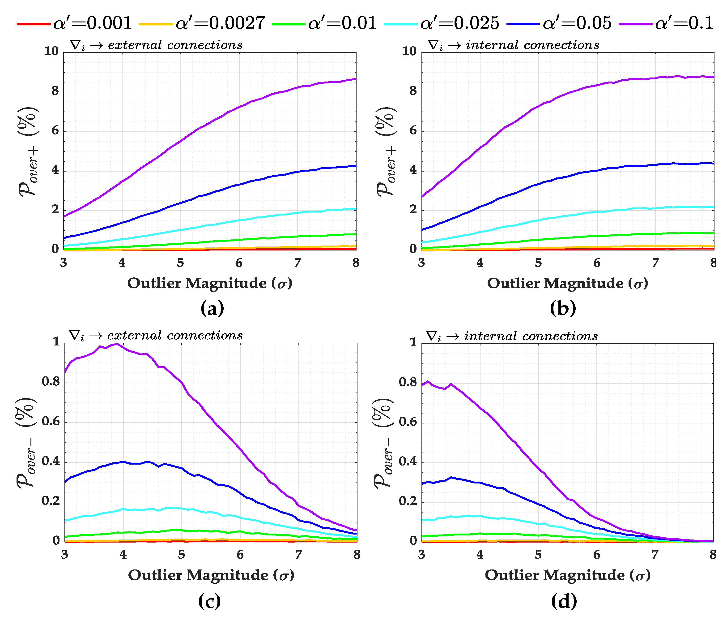
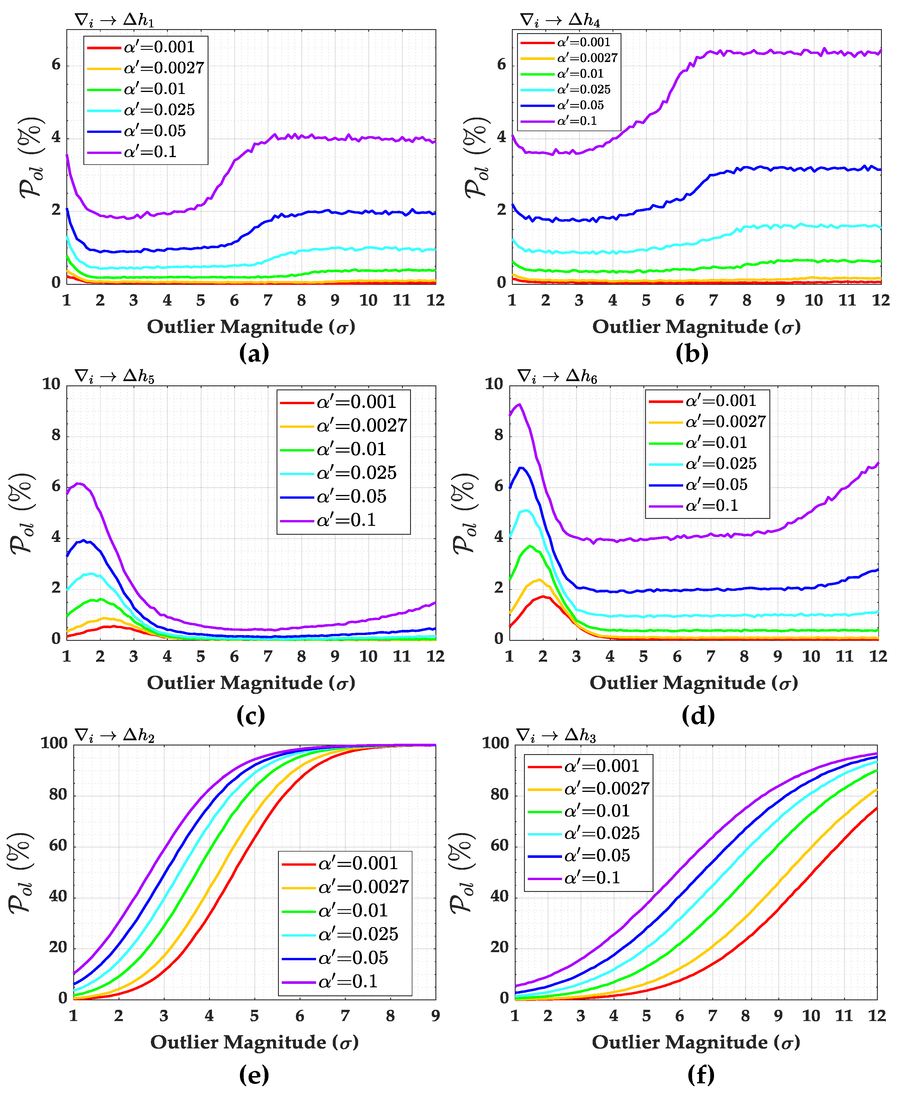
The over-identification cases ${\mathcal{P}}_{over+}$ and ${\mathcal{P}}_{over-}$ are presented in Figure 14. In general, the larger the Type I decision error ${\alpha }^{\prime }$, the larger the over-identification cases for that network. The larger the magnitude of the outlier, the larger the ${\mathcal{P}}_{over+}$ and smaller the ${\mathcal{P}}_{over-}$. For small ${\alpha }^{\prime }$, we observe that ${\mathcal{P}}_{over-}$ and ${\mathcal{P}}_{over+}$ are practically null (see, e.g., for ${\alpha }^{\prime }=0.001$ and ${\alpha }^{\prime }=0.0027$). In general, the larger the correlation coefficient ${\rho }_{{\mathit{w}}_{\mathit{i}},{\mathit{w}}_{\mathit{j}}}$, the smaller the ${\mathcal{P}}_{over+}$ and the larger the ${\mathcal{P}}_{over-}$. Moreover, we also observe that the larger the redundancy number $r_i$, the larger the ${\mathcal{P}}_{over+}$ and the smaller the ${\mathcal{P}}_{over-}$.

The probability of statistical overlap ${\mathcal{P}}_{ol}$ is practically null for this network. This is because each point of network (a) has at least four connections. This means that even with an exclusion, there are still three measurement levels per point (i.e., three connections per point), which guarantees the minimum redundancy necessary for the second round of IDS. The very low residual correlation of this network also contributes to the non-occurrence of statistical overlap.

The results presented so far are valid for the case of a system with high redundancy and low residual correlation. In the next section, we present the results for a system with low redundancy and high residual correlation.

6.2.2. Geodetic Network with High Correlation Between Residuals

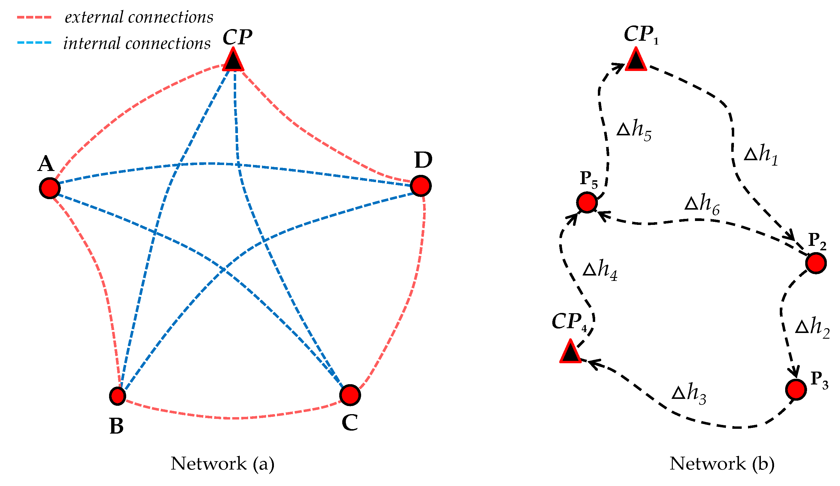
Now, the correlation between residuals is very high. This is the case for network (b) detailed in Figure 2. Since the measurements are correlated for network (b), instead of redundancy numbers, reliability numbers $\left({\overline{r}}_i\right)$ should be given as an internal reliability measure, as follows [43]:

$${\overline{r}}_i={\mathit{c}}_{\mathit{i}}^{\mathit{T}}{\mathit{Q}}_{\mathit{e}}{\mathit{c}}_{\mathit{i}}{\mathit{c}}_{\mathit{i}}^{\mathit{T}}\mathit{W}{\mathit{Q}}_{\widehat{\mathit{e}}}\mathit{W}{\mathit{c}}_{\mathit{i}},\forall i=1,\cdots ,n$$

(61)

The reliability numbers $\left({\overline{r}}_i\right)$ in Equation (61) are equivalent to redundancy numbers when it is assumed that the measurements are uncorrelated.

Table 7. Reliability numbers $\left({\overline{r}}_i\right)$, standard deviation ${\sigma }_{\Delta h_{i-j}}$ and standard deviation of estimated outlier ${\sigma }_{{\nabla }_i}$ for network (b).

$\Delta {\mathit{h}}_{\mathit{i}-\mathit{j}}$	${\overline{\mathit{r}}}_{\mathit{i}}$	${\mathit{\sigma }}_{\Delta {\mathit{h}}_{\mathit{i}-\mathit{j}}}$ (m)	${\mathit{\sigma }}_{{\mathit{\nabla }}_{\mathit{i}}}$ (m)
$\Delta h_1$	10.58	2.35	0.72
$\Delta h_2$	0.62	1.97	2.50
$\Delta h_3$	0.13	0.89	2.50
$\Delta h_4$	13.68	2.32	0.63
$\Delta h_5$	1.95	0.45	0.32
$\Delta h_6$	3.56	1.18	0.63

gives the reliability numbers $\left({\overline{r}}_i\right)$, the standard deviation of each measurement ${\sigma }_{\Delta h_{i-j}}$ and the standard deviation of each estimated outlier ${\sigma }_{{\nabla }_i}$ for network (b).

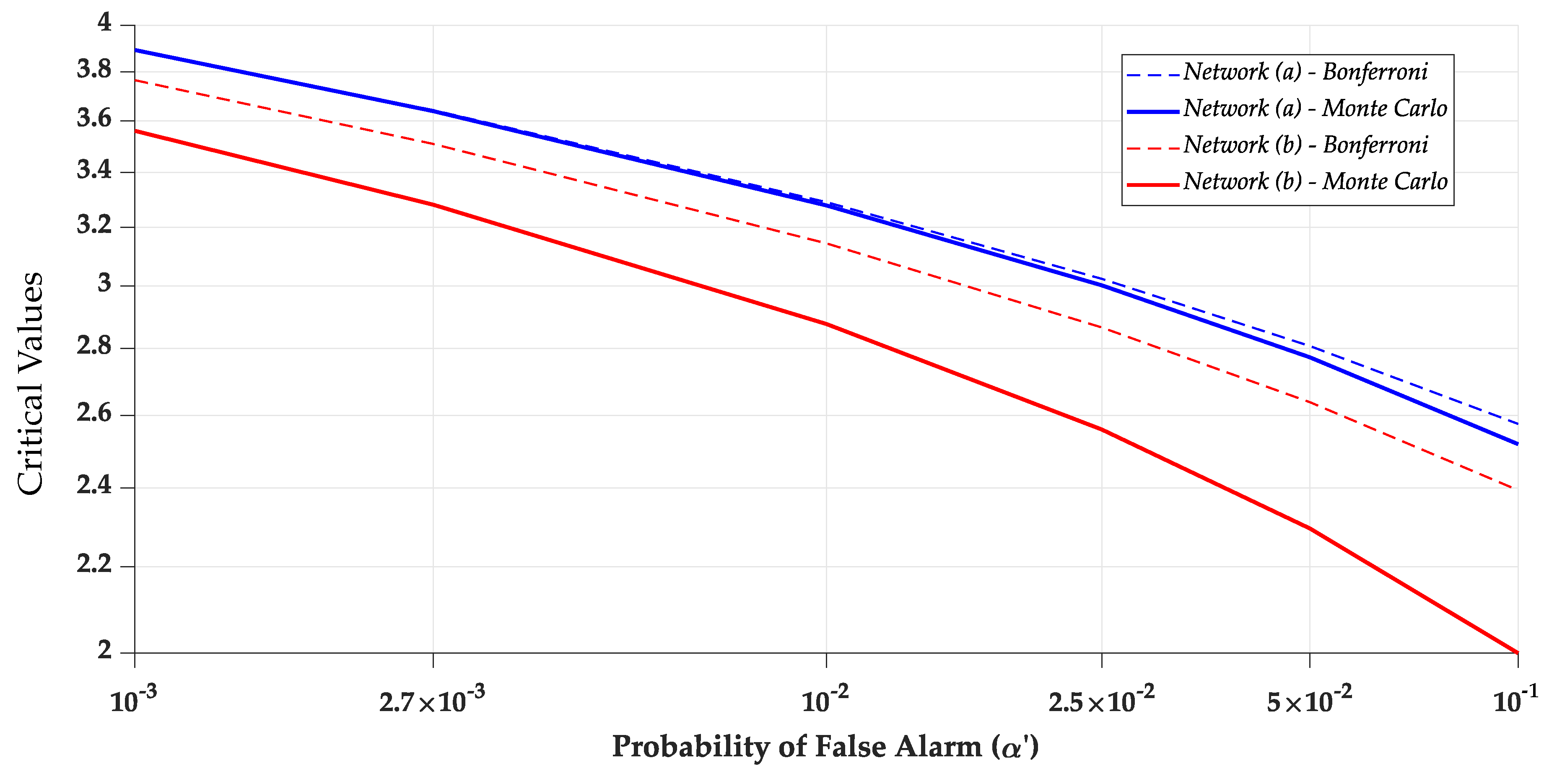
The probabilities of correct identification (${\mathcal{P}}_{CI}$) for this network are displayed in Figure 15. The critical values $(\widehat{k})$ for network (b) are those given in Table 4. The probability levels of correct detection (${\mathcal{P}}_{CD}$) are provided in Figure 16.

In contrast to network (a), the probability of correct identification (${\mathcal{P}}_{CI}$) for network (b) is different for each measurement. It is also found that the larger the Type I decision error ${\alpha }^{\prime }$, the higher the probability of correct identification (${\mathcal{P}}_{CI}$). However, it is only true up to a certain level of outlier magnitude. After this magnitude level, the larger the Type I decision error ${\alpha }^{\prime }$, the lower the probability of correct identification (${\mathcal{P}}_{CI}$).

The user-defined Type I error ${\alpha }^{\prime }$ has indeed become less significant at a certain outlier magnitude. Note, for example, that the probability of correct identification for measurement $\Delta h_1$ for ${\alpha }^{\prime }=0.1$ is higher than that for ${\alpha }^{\prime }=0.001$ when the outlier magnitude is between $1\sigma$ and $1.5\sigma$. For a magnitude greater than $1.5\sigma$, we note that the larger the Type I decision error ${\alpha }^{\prime }$, the lower the probability of correct identification ${\mathcal{P}}_{CI}$. The choice of Type I error ${\alpha }^{\prime }$, however, has no significant effect on the probability of correct identification ${\mathcal{P}}_{CI}$ for an outlier magnitude greater than $1.5\sigma$. This analysis can also be done with $\Delta h_4$, $\Delta h_5$ and $\Delta h_6$.

There is no probability of identification for both measurements $\Delta h_2$ and $\Delta h_3$. This is because the residual correlation of these measurements is equal to exactly one (i.e., ${\rho }_{{\mathit{w}}_{\mathit{i}},{\mathit{w}}_{\mathit{j}}}=1.00$). Furthermore, the reliability numbers $\left({\overline{r}}_i\right)$ in Table 7 for those measurements are close to zero. However, if one of those measurements were affected by a single outlier, then IDS would have the ability to detect it. In other words, there is reliability in terms of outlier detection for $\Delta h_2$ and $\Delta h_3$.

We observe that the higher the reliability numbers in Table 3, the higher the power of detection ${\mathcal{P}}_{CD}$ and identification ${\mathcal{P}}_{CI}$. In general, the larger the Type I decision error ${\alpha }^{\prime }$, the lower the probability of missed detection ${\mathcal{P}}_{MD}$ and, therefore, the higher the probability of correct detection ${\mathcal{P}}_{CD}$.

The sensitivity indicators MDB and MIB for $\Delta h_1$, $\Delta h_4$, $\Delta h_5$ and $\Delta h_6$ are shown in

Table 8. Relationship between the MDB and MIB for $\Delta h_1$ and for ${\tilde{\mathcal{P}}}_{CD}={\tilde{\mathcal{P}}}_{CI}=80\%$.

${\mathit{\alpha }}^{\prime }$	MIB	MDB	${\mathit{\lambda }}_{\mathit{q}=1}^{\left(\mathit{MIB}\right)}$	${\mathit{\lambda }}_{\mathit{q}=1}^{\left(\mathit{MDB}\right)}$	MIB/MDB
0.001	3.700$\sigma$	1.327$\sigma$	145.839	18.759	2.788
0.0027	3.700$\sigma$	1.240$\sigma$	145.839	16.380	2.984
0.010	3.750$\sigma$	1.109$\sigma$	149.807	13.102	3.381
0.025	3.840$\sigma$	1.009$\sigma$	157.084	10.846	3.806
0.050	3.980$\sigma$	0.930$\sigma$	168.747	9.214	4.280
0.100	4.320$\sigma$	0.830$\sigma$	198.810	7.339	5.205

,

Table 9. Relationship between the MDB and MIB for $\Delta h_4$ and for ${\tilde{\mathcal{P}}}_{CD}={\tilde{\mathcal{P}}}_{CI}=80\%$.

${\mathit{\alpha }}^{\prime }$	MIB	MDB	${\mathit{\lambda }}_{\mathit{q}=1}^{\left(\mathit{MIB}\right)}$	${\mathit{\lambda }}_{\mathit{q}=1}^{\left(\mathit{MDB}\right)}$	MIB/MDB
0.001	2.558$\sigma$	1.170$\sigma$	88.735	18.564	2.186
0.0027	2.566$\sigma$	1.093$\sigma$	89.291	16.201	2.348
0.010	2.598$\sigma$	0.982$\sigma$	91.532	13.077	2.646
0.025	2.659$\sigma$	0.895$\sigma$	95.902	10.863	2.971
0.050	2.784$\sigma$	0.820$\sigma$	105.107	9.118	3.395
0.100	3.082$\sigma$	0.738$\sigma$	128.771	7.390	4.174

,

Table 10. Relationship between the MDB and MIB for $\Delta h_5$ and for ${\tilde{\mathcal{P}}}_{CD}={\tilde{\mathcal{P}}}_{CI}=80\%$.

${\mathit{\alpha }}^{\prime }$	MIB	MDB	${\mathit{\lambda }}_{\mathit{q}=1}^{\left(\mathit{MIB}\right)}$	${\mathit{\lambda }}_{\mathit{q}=1}^{\left(\mathit{MDB}\right)}$	MIB/MDB
0.001	11.290$\sigma$	3.065$\sigma$	252.065	18.577	3.684
0.0027	11.260$\sigma$	2.863$\sigma$	250.727	16.209	3.933
0.010	11.315$\sigma$	2.565$\sigma$	253.183	13.011	4.411
0.025	11.360$\sigma$	2.328$\sigma$	255.201	10.717	4.880
0.050	11.530$\sigma$	2.127$\sigma$	262.896	8.947	5.421
0.100	11.940$\sigma$	1.906$\sigma$	281.925	7.184	6.264

and

Table 11. Relationship between the MDB and MIB for $\Delta h_6$ and for ${\tilde{\mathcal{P}}}_{CD}={\tilde{\mathcal{P}}}_{CI}=80\%$.

${\mathit{\alpha }}^{\prime }$	MIB	MDB	${\mathit{\lambda }}_{\mathit{q}=1}^{\left(\mathit{MIB}\right)}$	${\mathit{\lambda }}_{\mathit{q}=1}^{\left(\mathit{MDB}\right)}$	MIB/MDB
0.001	5.680$\sigma$	2.289$\sigma$	113.183	18.375	2.482
0.0027	5.700$\sigma$	2.134$\sigma$	113.981	15.976	2.671
0.010	5.695$\sigma$	1.908$\sigma$	113.781	12.769	2.985
0.025	5.825$\sigma$	1.729$\sigma$	119.035	10.492	3.368
0.050	6.021$\sigma$	1.579$\sigma$	127.180	8.747	3.813
0.100	6.394$\sigma$	1.409$\sigma$	143.426	6.965	4.538

, respectively. Both MIBs and MDBs were computed for each ${\alpha }^{\prime }$ and for a success rate of 0.8 (80%) for both outlier detection and identification, i.e., ${\tilde{\mathcal{P}}}_{CD}={\tilde{\mathcal{P}}}_{CI}=80\%$. The non-centrality parameters for outlier detection and identification were computed according to Equations (45) and (46), respectively. In general, the larger the Type I decision error ${\alpha }^{\prime }$, the larger the MIB and the smaller the MDB. In other words, the larger the Type I decision error ${\alpha }^{\prime }$, the greater the chances of outlier detection but the lower the chances of outlier identification. In that case, the larger the Type I Error ${\alpha }^{\prime }$, the larger the MIB/MDB ratio. Therefore, an outlier with a size of the MDB should be enlarged in order to identify it [1,2,12,46].

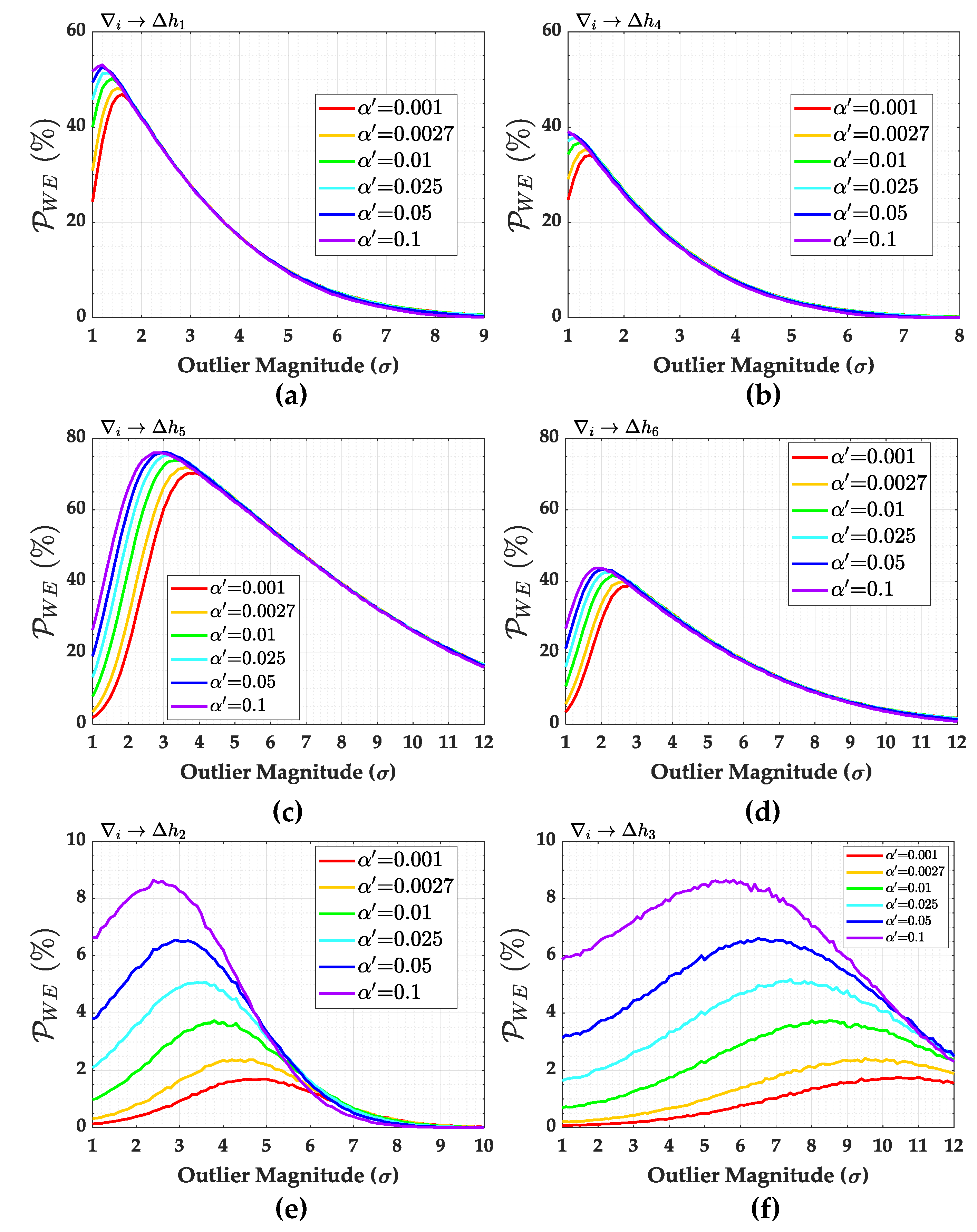
The overall probabilities of wrong exclusion (${\mathcal{P}}_{WE}$) for network (b) are provided in Figure 17. In general, we observe that the wrong exclusion rate (${\mathcal{P}}_{WE}$) increases up to a certain outlier magnitude and, from this point on, the wrong exclusion rate (${\mathcal{P}}_{WE}$) starts to decline, and the effect of the user-defined Type 1 decision error (${\alpha }^{\prime }$) on ${\mathcal{P}}_{WE}$ becomes neutral in practical terms. This effect is due to the residuals’ correlation. To see this effect more clearly, we also computed the individual contribution of each measurement to the overall wrong exclusion ${\mathcal{P}}_{WE}$ and their corresponding weighting factors given by Equations (40) and (41), respectively.

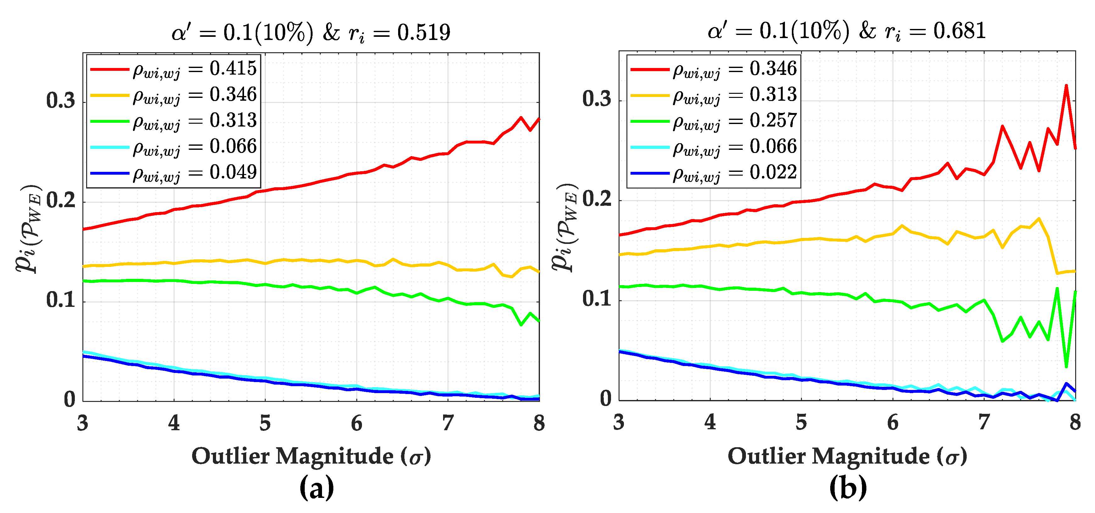
The individual contributions to the overall ${\mathcal{P}}_{WE}$ and their weighting factors for ${\alpha }^{\prime }=0.1$ are displayed in Figure 18 and Figure 19, respectively. It is important to mention that the behaviour shown in Figure 18 and Figure 19 is similar to that for other ${\alpha }^{\prime }$ values. We observe that the correlation coefficient (${\rho }_{{\mathit{w}}_{\mathit{i}},{\mathit{w}}_{\mathit{j}}}$) only has a direct relationship with ${\mathcal{P}}_{WE}$ for a certain outlier magnitude. Let us consider the case in which $\Delta h_6$ is set up as an outlier. In that case, the larger the correlation coefficient (${\rho }_{{\mathit{w}}_{\mathit{i}},{\mathit{w}}_{\mathit{j}}}$), the higher the individual contribution to ${\mathcal{P}}_{WE}$. Of course, this only holds true if the outlier magnitude is larger than $3.2\sigma$. This is also evident from the results of the weighting factors in Figure 19.

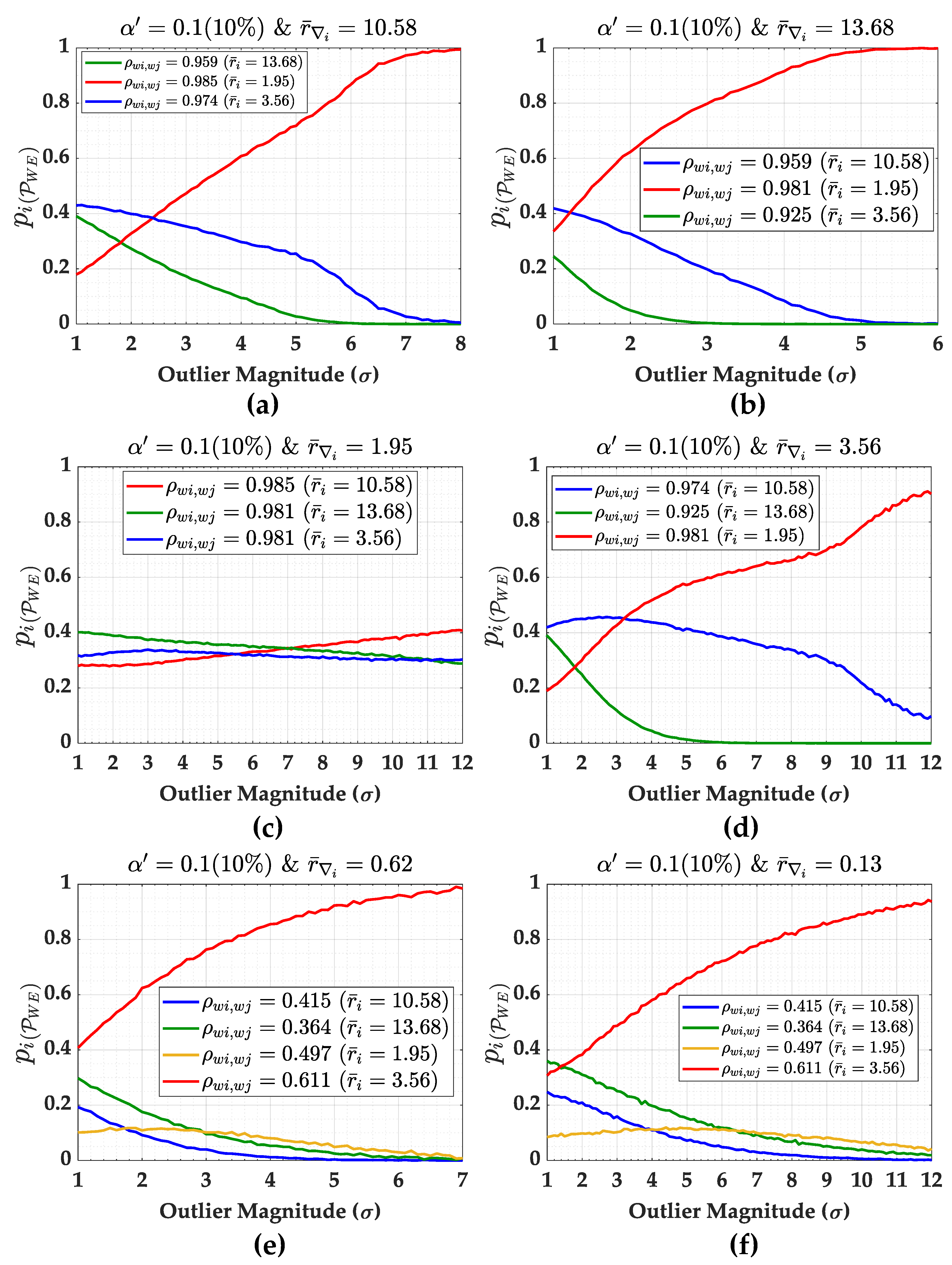
An important highlight is the association between the MIB and the contribution of each measurement to the probability of wrong exclusion ${\mathcal{P}}_{WE}$ in Figure 18.

We observe that it is possible to find the value of the MIB at high success rates when the individual contributions to the overall wrong exclusion ${\mathcal{P}}_{WE}$ of a given outlier start to decrease simultaneously. It is important to mention that this simultaneous decay occurs when there is a direct relationship between the correlation coefficient (${\rho }_{{\mathit{w}}_{\mathit{i}},{\mathit{w}}_{\mathit{j}}}$) and the wrong exclusion rate ${\mathcal{P}}_{WE}$. In that case, the identifiability of a given outlier can be verified for a given significance level ${\alpha }^{\prime }$ and probability of correct identification ${\mathcal{P}}_{CI}$.

Figure 20 illustrates an example for measurements $\Delta h_1$ and $\Delta h_4$. The black dashed line corresponds to the probability of correct identification ${\mathcal{P}}_{CI}$ and the respective MIB for ${\alpha }^{\prime }=0.001$. Note that when the effect of all measurements on ${\mathcal{P}}_{WE}$ decreases, it is possible to find an outlier magnitude that can be identified. In other words, the effect of the correlation between residuals (${\rho }_{{\mathit{w}}_{\mathit{i}},{\mathit{w}}_{\mathit{j}}}$) becomes insignificant at a certain outlier magnitude, which increases the probability of identification.

The probabilities of wrong exclusion for both $\Delta h_2$ and $\Delta h_3$ are smaller than those for the other cases. This is because of the correlation between residuals (${\rho }_{{\mathit{w}}_{\mathit{i}},{\mathit{w}}_{\mathit{j}}}$). In fact, we also note that although there is no reliability in terms of outlier identification for cases in which the correlation is ${\rho }_{{\mathit{w}}_{\mathit{i}},{\mathit{w}}_{\mathit{j}}}=1.00$ (i.e., 100%), there is reliability for outlier detection. In this case, outlier detection is caused by overlapping w-test statistics. The result for statistical overlap (${\mathcal{P}}_{ol}$) is displayed in Figure 21. In general, the larger the Type 1 decision error ${\alpha }^{\prime }$, the larger the statistical overlap (${\mathcal{P}}_{ol}$).

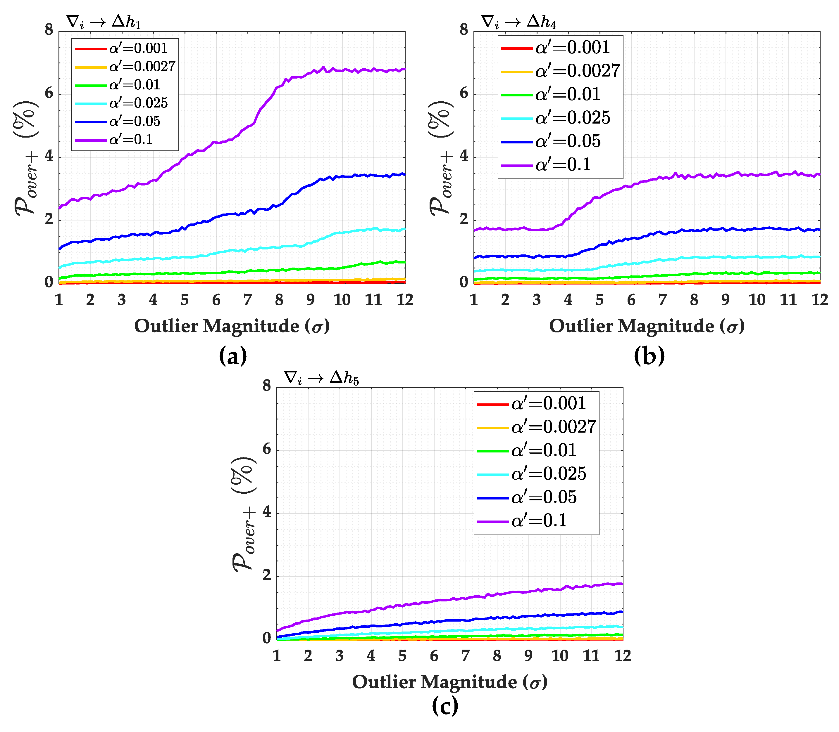
The over-identification cases (${\mathcal{P}}_{over+}$ and ${\mathcal{P}}_{over-}$) are displayed in Figure 22 and Figure 23, respectively. We observe that the larger the Type I decision error (${\alpha }^{\prime }$), the larger the over-identification cases. It should be noted that ${\mathcal{P}}_{over+}$ is always larger than ${\mathcal{P}}_{over-}$. Over-identification ${\mathcal{P}}_{over-}$ is practically null. The over-identification cases ${\mathcal{P}}_{over+}$ for $\Delta h_2$, $\Delta h_3$ and $\Delta h_6$ and ${\mathcal{P}}_{over-}$ for $\Delta h_1$ are exactly null. The over-identifications ${\mathcal{P}}_{over-}$ for $\Delta h_2$ and $\Delta h_3$ are less than 0.2% and are therefore not shown here.

7. Conclusions and Outlook

In this paper, we propose a procedure to compute the probability levels associated with an iterative outlier elimination procedure. This iterative outlier elimination procedure is known among geodesists as iterative data snooping IDS. On the basis of the probability levels of IDS, the sensitivity indicators—the Minimal Detectable Bias (MDB) and Minimal Identifiable Bias (MIB)—can also be determined for a given measurement system.

We emphasize that the probability levels associated with IDS in the presence of an outlier were analysed as a function of the user-defined Type I decision error (${\alpha }^{\prime }$), outlier magnitude (${\nabla }_i$), correlation between test statistics (${\rho }_{{\mathit{w}}_{\mathit{i}},{\mathit{w}}_{\mathit{j}}}$) and reliability indicators (i.e., redundancy number $r_i$ and reliability number ${\overline{r}}_i$). It is important to highlight that these probability levels are based on critical values that were optimized via Monte Carlo.

We highlight the main findings of the paper below:

• If one adopts the Bonferroni correction to compute the critical value of the test statistic associated with IDS, one does not have control over Type I decision errors. This is only true for small ${\alpha }^{\prime }$ values and for a measurement system with high redundancy and a low correlation between test statistics.
• If one maintains the condition of a measurement system with a low correlation between test statistics, the probability of wrong exclusion ${\mathcal{P}}_{WE}$ is too low. In that case, one should opt for a larger ${\alpha }^{\prime }$ so that the probability of missed detection ${\mathcal{P}}_{MD}$ is as small as possible. Thus, it is possible to guarantee a high outlier identification rate. However, we verify that, under certain circumstances, the larger the Type I decision error ${\alpha }^{\prime }$, the higher the probability of correct detection ${\mathcal{P}}_{CD}$ but the lower the probability of correct identification ${\mathcal{P}}_{CI}$. In that case, the larger the Type I Error ${\alpha }^{\prime }$, the larger the ratio between the sensitivity indicators MIB/MDB.
• The larger the Type I error (${\alpha }^{\prime }$), the higher the probability of correct outlier identification (${\mathcal{P}}_{CI}$). However, it is valid only to a certain limit of outlier magnitude (threshold). There is an inversion when the outlier magnitude is greater than this threshold: i.e., the larger the ${\alpha }^{\prime }$, the lower the ${\mathcal{P}}_{CI}$. This is more critical in the case of a measurement system with a high correlation between test statistics. Moreover, the Type I decision error ${\alpha }^{\prime }$ restricts the maximum rate of ${\mathcal{P}}_{CI}$.
• We also observe that it is possible to find the value of the MIB when the contributions of each measurement to the probability of wrong exclusion ${\mathcal{P}}_{WE}$ start to decline simultaneously. In that case, the identifiability of a given outlier can be verified for a given ${\alpha }^{\prime }$ and ${\mathcal{P}}_{CI}$. In other words, for a certain outlier magnitude, the effect of the correlation between test statistics becomes insignificant, which increases the probability of identification. Moreover, if a small outlier magnitude (outlier with a magnitude close to the measurement uncertainty) were to arise for a measurement system with a high correlation between test statistics, the alternative hypotheses would not be distinguished; i.e., this outlier would never be identified.
• The larger the Type I decision error ${\alpha }^{\prime }$, the larger the over-identification cases. The over-identification case ${\mathcal{P}}_{over+}$ is always larger than ${\mathcal{P}}_{over-}$. We also note that the lower the correlation between test statistics, the higher the probability of over-identification positive ${\mathcal{P}}_{over+}$. For small ${\alpha }^{\prime }$ (close to ${\alpha }^{\prime }=0.001$), ${\mathcal{P}}_{over-}$ is practically null.
• When the correlation between two test statistics is equal to exactly 1.00, ${\mathcal{P}}_{CI}$ does not exist, but there is ${\mathcal{P}}_{CD},$ which is mainly caused by ${\mathcal{P}}_{ol}$.

The computation procedure presented in this paper was successfully applied to a practical example of geodetic networks. Although the procedure was applied to geodetic networks, it is a generally applicable method. The authors have been working on solutions to find a relationship between the variables computed deterministically (e.g., local redundancy, residuals’ correlation) with the probability levels computed by Monte Carlo. The use of Monte Carlo will no longer be needed to find the MIB if a model is found. Moreover, further investigation is required to apply this analysis to general problems with multiple outliers.