Impact of Fire Emissions on U.S. Air Quality from 1997 to 2016–A Modeling Study in the Satellite Era


1
Universities Space Research Association, Columbia, MD 21046, USA
2
NASA Goddard Space Flight Center, Greenbelt, MD 20771, USA
3
Department of Atmospheric & Oceanic Science, University of Maryland, College Park, MD 20742, USA
4
Earth System Science Interdisciplinary Center, University of Maryland, College Park, MD 20740, USA
5
NOAA Air Resources Laboratory, College Park, MD 20740, USA
6
Center for Spatial Information Science and Systems, George Mason University, Fairfax, VA 22030, USA
*
Authors to whom correspondence should be addressed.
Remote Sens. 2020, 12(6), 913; https://doi.org/10.3390/rs12060913
Submission received: 7 January 2020
/
Revised: 3 March 2020
/
Accepted: 5 March 2020
/
Published: 12 March 2020
(This article belongs to the Special Issue Remote Sensing of Biomass Burning)
Abstract
:A regional modeling system that integrates the state-of-the-art emissions processing (SMOKE), climate (CWRF), and air quality (CMAQ) models has been combined with satellite measurements of fire activities to assess the impact of fire emissions on the contiguous United States (CONUS) air quality during 1997–2016. The system realistically reproduced the spatiotemporal distributions of the observed meteorology and surface air quality, with a slight overestimate of surface ozone (O3) by ~4% and underestimate of surface PM2.5 by ~10%. The system simulation showed that the fire impacts on primary pollutants such as CO were generally confined to the fire source areas but its effects on secondary pollutants like O3 spread more broadly. The fire contribution to air quality varied greatly during 1997-2016 and occasionally accounted for more than 100 ppbv of monthly mean surface CO and over 20 µg m−3 of monthly mean PM2.5 in the Northwest U.S. and Northern California, two regions susceptible to frequent fires. Fire emissions also had implications on air quality compliance. From 1997 to 2016, fire emissions increased surface 8-hour O3 standard exceedances by 10% and 24-hour PM2.5 exceedances by 33% over CONUS.
1. Introduction
In the past few decades, wildfires have occurred more frequently with longer durations in the western U.S. [1,2]. Wildfires not only wreak property damages and threaten human lives on their pathway, but also deteriorate local/regional air quality and pose imminent risks to both human and ecosystem health [3,4,5,6]. For example, case studies have shown that wildfires have caused large exceedances of ambient PM2.5 (particulate matter with aerodynamic diameter equal to or less than 2.5 µm) standard in downwind areas [7,8,9,10,11] and contributed substantially to ambient ozone (O3) pollution over the U.S. [12,13,14,15,16,17]. Under the Intergovernmental Panel on Climate Change’s (IPCC) A1B and A2 scenarios, the researchers [18,19] project that the U.S. wildfire activities would increase toward the middle of the 21st century. In anticipation of continuing decreases in anthropogenic emissions in the U.S., Jacob and Winner [20] suggest that fire emissions would be more important to regulate future U.S. air quality. Meanwhile, aerosols emitted by fires and other sources can exert impacts on local/regional climate through complex aerosol-cloud-radiation interactions [21,22,23] that in turn affects U.S. air quality [24,25,26].
Investigation of the effects of fire emissions on U.S. air quality with air quality models (AQM) has emerged recently [27,28,29,30]. However, these studies either focused on isolated fire events [28,29] or the fire season in specific years [27,30]. Systematic evaluation of impacts of fire emissions on U.S. air quality over decadal time horizon is lacking. Taking advantage of the satellite observations of fire activities in the past 20 years, this study used a state-of-the-art modeling system to quantify the effects of fire emissions on U.S. air quality as well as pollution extremes.
2. Experiment Design
2.1. The Regional Modeling System
The state-of-the-art modeling system used here integrates three major components—a regional climate model (RCM), an emissions processing model (EPM), and an AQM. The RCM has been developed from the community Weather Research and Forecasting (WRF) [31] model with extensive improvements of many physical representations, including but not limited to, land-atmosphere-ocean interactions, cloud microphysics and convection, aerosol and radiation, which makes it a suitable tool for seamless applications to regional weather and climate prediction [32,33]. Hereafter, it is referred to as the Climate extension of WRF (CWRF), which has been extensively evaluated against observations and demonstrated good skills in capturing characteristics of U.S. regional temperature and precipitation [34,35,36,37,38,39]. It thus can provide realistic meteorology and regional climate needed to drive AQM.
The EPM is the Sparse Matrix Operator Kernel Emissions (SMOKE) version 3.7 (https://www.cmascenter.org/smoke/) [40]. It allocated the emissions from on-road, off-road, and area sources to the surface layer of each model grid using the spatial surrogate auxiliary data. Emissions from point sources (e.g., stacks from power plants) were distributed vertically based on stack height and plume rise that was calculated with the method by Briggs [41]. The gridded emissions were then split into model species based on the chosen chemical mechanism. Many model species, e.g., numerous organic compounds, were not directly included in the emission inventory. Instead, the volatile organic compound (VOC) was reported. In order for it to be useful in the model, VOC must be broken into the species the model can recognize. The breakage of VOC followed the preset factors based on the chemical mechanism utilized in the model. Subsequently, the gridded model species were allocated to each time step using the source-specific temporal profiles.
The AQM is the Community Multiscale Air Quality (CMAQ) version 5.2 [42]. It is driven by the SMOKE-analyzed emissions and the CWRF-generated meteorological fields through the modified meteorology-chemistry interface processor (MCIP) version 4.3 [43]. The carbon bond version 6 (CB06) mechanism for gases and AERO5 scheme for aerosols have been chosen in this study. As a backbone to the National Air Quality Forecast Capability (NAQFC) modeling system that provides daily U.S. national air quality forecast, CMAQ has vigorously been evaluated [44,45,46,47].
2.2. Emissions Preparation
The National Emission Inventory 2011 (NEI2011) was adopted to create the baseline (2014) anthropogenic emissions with modifications using measurements from the Ozone Monitoring Instrument (OMI) onboard Aura satellite, the ground-based national Air Quality System (AQS), and the in-situ continuous emissions monitoring in power plants [48]. The Air Pollutant Emissions Trends Data compiled by the U.S. Environmental Protection Agency (EPA) (https://www.epa.gov/air-emissions-inventories/air-pollutant-emissions-trends-data) were then used to adjust the modified NEI2011 data into each simulation year with the factors scaled to the baseline emissions. In areas with no NEI2011 data, the Emissions Database for Global Atmospheric Research (EDGAR v3, http://edgar.jrc.ec.europa.eu/) at a 1 by 1 degree resolution developed by the Joint Research Centre of European Commission was projected to the domain and merged with the NEI2011 data.
The fire emissions were based on the Global Fire Emissions Database with small fires, version 4 (GFEDv4s), which was derived, in combination with the ancillary data of carbon pools, emissions factors, and combustion completeness, from the satellite measurements of burnt areas by the Moderate Resolution Imaging Spectroradiometer (MODIS) or the Visible Infrared Scanner (VIRS) and Along-Track Scanning Radiometer (ATSR) in the pre-MODIS era [49,50]. The major improvement of GFEDv4s over the previous versions was that it contained emissions from small fires that were derived by combining the measurements of 500 m resolution burnt area, 1 km resolution thermal anomalies for active fires, and 500 m resolution surface reflectance. The 0.25-degree resolution GFEDv4s data were projected onto the regional domain grids and split into the CB06 and AERO5 species. The GFEDv4s had a monthly resolution prior to year 2000 and daily one onward. A program was developed to merge the aforementioned anthropogenic and fire emissions into the temporalized, gridded, and speciated data ready for CMAQ.
The biogenic emissions were calculated online within CMAQ from the gridded normalized vegetation emissions under the standard condition (303 K and 1,000 μmol m−2 s−1 of photosynthetic active radiation) produced by SMOKE with the Biogenic Emissions Landuse Database version 3 (BELD3, https://www.epa.gov/air-emissions-modeling/biogenic-emissions-landuse-database-version-3-beld3). BELD3 contained 230 vegetation classes at a 1-km resolution covering most of North America, which were processed through the spatial allocator developed by Community Modeling and Analysis System (CMAS) (https://www.cmascenter.org/sa-tools/) to generate the gridded vegetation distribution map ready for SMOKE. An ancillary file was also developed to facilitate the CMAQ online calculation of sea salt emissions.
2.3. Experiment Set-Up
Two sets of 20-year (1997–2016) simulations were carried out, with one set including and the other excluding fire emissions. All other model configurations were kept identical for both experiments. The study domain covered the contiguous United States (CONUS), southern Canada, northern Mexico, and the adjacent oceans with a 30-km horizontal grid. Due to the computational constrain, a higher than 30-km resolution modeling was not possible for this study. However, the 30-km resolution simulation has been proven to realistically capture the spatial-temporal distributions of temperature and precipitation, including extreme events [32,51], which is important to an accurate air quality simulation. In addition, the 30-km grid is comparable to the 0.25-degree resolution of GFEDv4s fire emissions data. Therefore, the 30-km resolution modeling was appropriate for the scope of this study.
The CWRF control physics configuration was utilized in this investigation. This included the long- and short-wave radiation scheme of Chou and Suarez [52] and Chou et al. [53], cloud microphysics scheme of Tao et al. [54], the ensemble cumulus parameterization of Qiao and Liang [35,36,37], the planetary boundary layer scheme of Holtslag and Boville [55], and the Conjunctive Surface-Subsurface Process model (CSSP) predicting detailed terrestrial hydrology and land-atmosphere interaction developed by Liang’s group over years [56,57,58,59,60,61,62]. The large-scale meteorology conditions driving CWRF were derived from the European Centre for Medium-Range Weather Forecast Interim reanalysis (ERI) [63]. The chemical initial and boundary conditions were obtained from the climatological profiles built in CMAQ.
3. Results
3.1. Fire Emissions During 1997–2016
Figure 1a shows the evolution of fire emission from 1997 to 2016 over the study domain. It was readily seen that the inter-annual variations of fire emissions were large. Relative to the baseline year (2014), fire emissions in 16 other years were higher. The particularly strong fire years were 2002 and 2013 with emissions more than 3 times of those in 2014. On the other hand, 2001 and 2004 experienced lower fire emissions than 2014, while 2016 was on par with the baseline.
Figure 1b displays the ratios of major air pollutants from fires to those from anthropogenic emissions over 1997-2016. In general, fire emissions only accounted for a small portion (less than 5%) of the respective anthropogenic emissions of SO2, NOx, and NH3. The fire contributions to CO and black carbon (BC) became more prominent, frequently accounting for more than 10% of the annual man-made emissions. Fire was a major source of organic carbon (OC) with over 50% of anthropogenic emissions in 11 of 20 years between 1997 and 2016. In the strong fire years of 2002 and 2013, OC emissions from fires were 14% and 19% higher than those from man-made sources, respectively.
It is worth noting that the steady decreases in anthropogenic emissions, especially of CO, SO2, and NOx, have made fire more important an emission source over the years. For example, annual fire emissions of CO, SO2, and NOx were similar (approximately 5% in difference) between 1998 and 2011. Meanwhile, the 2011 anthropogenic emissions of CO, SO2, and NOx were 44%, 66%, and 41% lower than the respective 1998 ones. This increased the ratio of fire to anthropogenic emissions from 9.9% in 1998 to 16.9% in 2011, a nearly 70% jump for CO. The ratios for SO2 and NOx increased from 0.9% and 2.6% in 1998 to 2.6% and 4.0% in 2011, respectively. If the current decreasing trend of anthropogenic emissions continues, fire emissions are anticipated to account for more percentage of total emissions and their role in regulating air quality will become more important in the future.
Though fire occurred at varying locations in different years, some regions were more susceptible to fires as illustrated in Figure 2. The southeastern U.S. (boxed on panel (a) of Figure 2), Northern California (boxed on panel (c)), and the northwestern U.S. (boxed on panel (d)) repeatedly experienced fire hazards. Therefore, these three regions were selected for detailed analysis of fire impact on regional air quality.
3.2. Evaluation of CWRF and CMAQ
The CWRF simulated 2-meter temperature (T2) and precipitation were compared to the respective observations to evaluate the model ability in reproducing the meteorology conditions. The T2 and precipitation observations were derived from the quality-controlled records of 8,516 stations in the National Weather Service (NWS) Cooperative Observer network [64,65]. The daily precipitation data were adjusted for topographic dependence using monthly mean data from the Parameter elevation Regression on Independent Slopes Model (PRISM) by Daly et al. [66] to correct the observation bias for mountain sites [67]. The station data were then mapped onto the CWRF grid following the mass-conservation Cressman [68] objective analysis method [67].
Figure 3 illustrates the biases of T2 (top panels) and precipitation (bottom panels) over CONUS for winter (DJF), spring (MAM), summer (JJA), and fall (SON) based on the 20-year average. In winter, CWRF underestimated T2 in the northwestern U.S. and overestimated it in the Great Plains with typical biases within ±2 K. In spring, the underestimate was generally weakened while the overestimate was enhanced by 0.5 - 1 K. In summer, CWRF generally overestimated T2 across CONUS except in the Gulf States, with the largest biases of 3-4 K occurring along the coastal California as well as large portions of Iowa and Nebraska. In autumn, such overestimates were reduced to below 3 K and limited in the central to northern Great Plains. Overall, the biases in CONUS were -0.06, 0.68, 1.62, and 0.92 K for winter, spring, summer, and autumn, respectively. The corresponding root mean square error (RMSE) were 1.51, 1.33, 1.96, and 1.34 K, and the spatial pattern correlations with observations were high (> 0.97) for all seasons.
CWRF also performed well in reproducing precipitation, having the spatial pattern correlations with observations larger than 0.89 for all seasons. Its biases were typically within ±0.5 mm day−1 in most regions of CONUS and for all seasons. Major exceptions included overestimates of 0.5-1 mm day−1 in the states around the Great Lakes in winter, which were expanded to cover the Midwest and northern Great Plains in spring and turned to underestimates of a same magnitude in the central U.S. in summer. Larger biases occurred in some small regions, including the western mountainous areas (where observations were scarce) in winter, spring and autumn, as well as southern Texas and Florida in summer and autumn (when tropical storms prevailed). Overall, the biases were 0.16, 0.26, -0.19, and -0.06 mm day−1 for winter, spring, summer, and autumn, respectively. The corresponding RMSEs were 0.75, 0.66, 0.52, and 0.55 mm day−1. Therefore, CWRF realistically reproduced the T2 and precipitation distributions.
The CMAQ simulation was evaluated against the ground observations archived in AQS managed by U.S. EPA (https://www.epa.gov/outdoor-air-quality-data). The measured hourly surface air quality data at the monitoring sites were processed using the EPA Remote Sensing Information Gateway (RSIG) processor (https://www.epa.gov/hesc/remote-sensing-information-gateway) and mapped onto the CMAQ grid. The detailed description of CMAQ model evaluations can be found in He et al. [69], who investigated the long-term trends of O3 pollution observed by the AQS and modeled by the CWRF-CMAQ system, focusing on the summer season. Here only an overview CMAQ evaluation was provided.
Figure 4 displays the scatter density plots of the comparison of annual-mean surface O3 and PM2.5 between modeled and measured results paired in time and space from 2000 to 2016. CMAQ slightly overestimated surface O3, with the normalized mean bias (NMB) of 4.07% and RMSE of 5.31 ppbv. It well captured the observed surface O3 spatiotemporal variations, with a correlation coefficient of 0.52. CMAQ slightly underestimated surface PM2.5 with NMB of approximately -9.8%. Its RMSE was 3.83 µg m−3 and correlation coefficient with observations was around 0.41. However, zooming into the fire susceptible sub-regions as highlighted in Figure 2, the NMB became larger in magnitudes. For example, the NMBs for PM2.5 were -39.6%, -47.7%, and -58.1% for the northwestern U.S., Northern California, and the southeastern U.S., respectively, approximately 4.0, 4.9, and 5.9 times of the NMB over CONUS. This might come from the uncertainty of fire emissions. Based on a recent study by Pan et al. (2020) who compared the six commonly used biomass burning emissions inventories, GFEDv4s had the smallest fire emissions over the temperate North America. The usage of other fire emissions inventories may improve CMAQ performance over CONUS. In addition, the potential misrepresentation of plume height might mistakenly allocate fire emissions at wrong altitudes. In the future, the fire emissions inventory with plume height information will greatly help in accurate simulations of fire-related air quality.
3.3. Fire Contribution to Air Quality
3.3.1. Average Air Quality
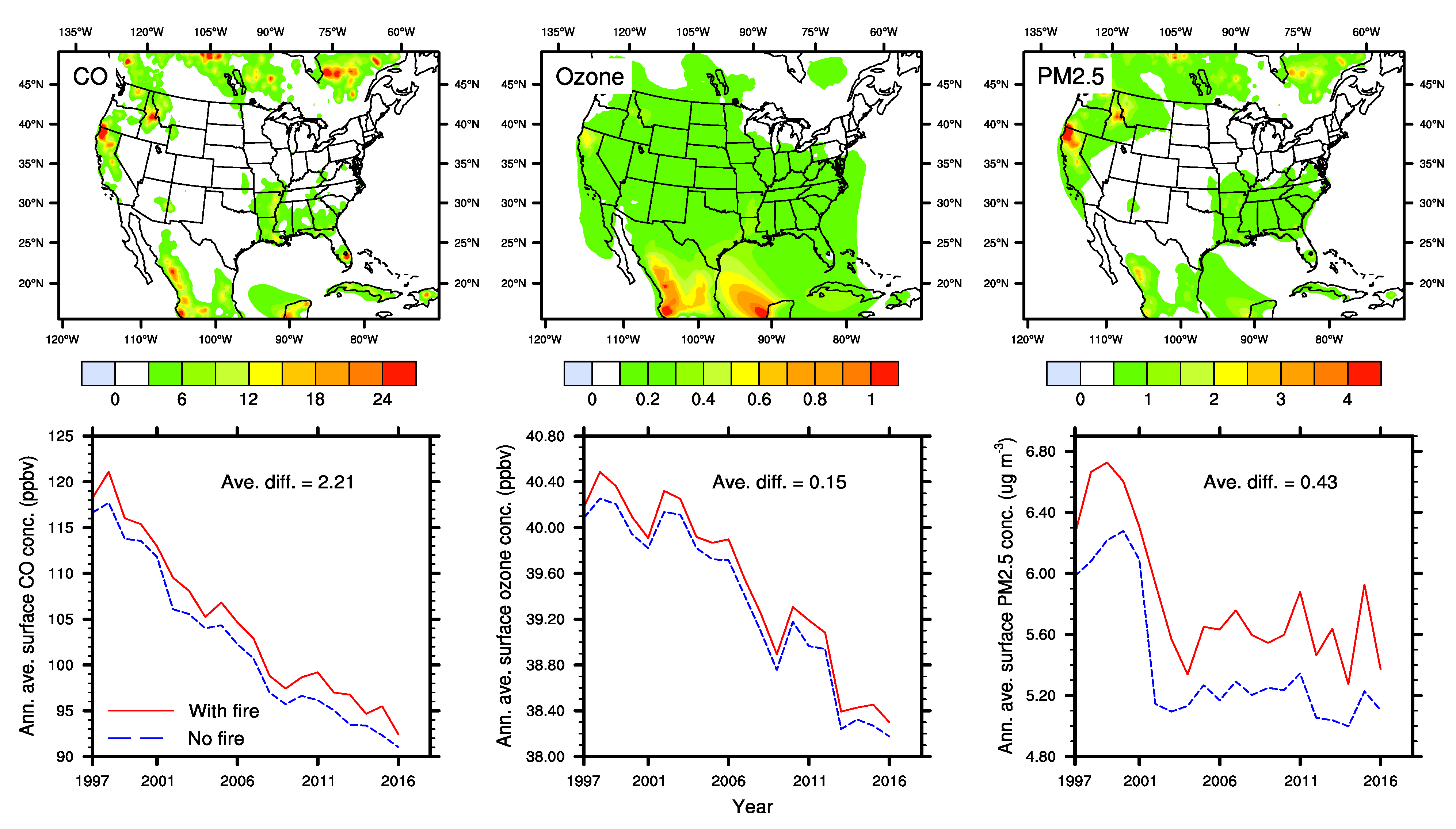
The fire contributions were obtained by the differences between the CMAQ results with and without fire emissions. Figure 5 (top panels) displays the 20-year average contributions of fire emissions to surface air quality of CO, O3, and PM2.5. In general, the impacts on primary pollutants such as CO were typically at or close to fire locations, including Canada, the northwestern U.S., northern California, southeastern U.S., west coastal areas, and Yucatan Peninsula of Mexico. The 20-year mean fire contribution to surface CO level reached more than 20 ppbv in certain regions, with the domain average as 2.21 ppbv. On the other hand, the impacts on secondary pollutants (chemically formed in the atmosphere from precursor species) such as O3 and PM2.5 (which has both primary and secondary origins) spread into broader areas and far away from fire source locations. For example, fires led to more than 0.2 ppbv increase in average surface O3 concentrations across most of the domain with the largest enhancement reaching 1 ppbv. Averaged over the entire domain, the 20-year mean surface O3 and PM2.5 levels were enhanced by 0.15 ppbv and 0.43 µg m−3, respectively, due to fire activities.
Figure 5 (bottom panels) shows the inter-annual variations of domain-average annual-mean surface CO, O3, and PM2.5 levels from 1997 to 2016. Both CO and O3 displayed significant descending trends over the years, whereas surface PM2.5 level stabilized from the mid-2000s after an initial decrease from late 1990s to mid-2000s. These trends were in line with the anthropogenic emissions changes over the period as shown in the U.S. EPA’s National Air Pollutant Emissions Trends. As expected, the fire contributions to surface air quality varied largely from year to year. For example, fires increased the domain-average annual-mean surface CO level by 3.44 ppbv in 1998, the largest within 20 years, and by 1.16 ppbv in 2001, the smallest of the period. The fire contributions to surface O3 and PM2.5 ranged from 0.09 to 0.23 ppbv and from 0.21 to 0.79 µg m−3, respectively.
Three regions susceptible to fires, as shown on Figure 2, were selected for analyzing the time evolution of fire effects on regional air quality. Figure 6 displays the time series of the contributions of fire emissions to surface CO, O3, and PM2.5 levels over these regions. As anticipated, fire contributed heavily to local air quality where it occurred, such as the northwestern U.S., Northern California, and the southeastern U.S. The monthly maximum contributions to surface CO, O3, and PM2.5 concentrations could reach 210 ppbv, 4.9 ppbv, and 44 µg m−3, respectively, in the northwestern U.S.; and 150 ppbv, 5.1 ppbv, and 48 µg m−3 in Northern California. The 20-year average fire contributions to surface CO, O3, and PM2.5 levels were 7.07 ppbv, 0.26 ppbv, and 1.68 µg m−3, respectively, in Northern California, which were 3.2, 1.7, and 3.9 times of the domain-mean contributions. In the northwestern U.S., the fire emissions accounted for 6.86 ppbv, 0.24 ppbv, and 1.40 µg m−3 of surface CO, O3, and PM2.5 concentrations, respectively.
The fire emissions from the southeastern U.S. were relatively lower but generally more persistent than those from the northwestern U.S. and Northern California. As a result, the peak fire contributions to surface CO, O3, and PM2.5 concentrations were approximately 20 ppbv, 1.6 ppbv, and 5 µg m−3, respectively, while the corresponding 20-year averages were 4.25 ppbv, 0.24 ppbv, and 0.75 µg m−3. The peak-to-average ratios for CO, O3, and PM2.5 were 4.7, 6.7, and 6.7, respectively, in the southeastern U.S., much lower than the corresponding ratios, which were at least 20, in the northwestern U.S. and Northern California.
3.3.2. Extreme Air Quality
Investigation of fire emission effect on extreme air quality has regulatory importance. Here the extreme air quality was defined as the surface pollutant concentration exceeding the corresponding National Ambient Air Quality Standards (NAAQS). According to U.S. EPA, two criteria pollutants, O3 and PM2.5, constantly exceed the respective NAAQS and plague public health in many counties in the U.S. Currently, the NAAQS is 70 ppbv for O3 averaged over 8 hours and 35 µg m−3 for PM2.5 averaged over 24 hours (https://www.epa.gov/criteria-air-pollutants/naaqs-table). As of 2019, there have been 197 counties designated as O3 nonattainment (exceeding NAAQS) with more than one third of total U.S. population residing in those counties. Meanwhile, there have been 16 counties designated as PM2.5 nonattainment with over 20 million people suffering from the heavy PM2.5 pollution (https://www.epa.gov/green-book). Therefore, the following analysis would focus on O3 and PM2.5.
Figure 7 shows the probability distributions of surface 8-hr average O3 and 24-hr average PM2.5 over CONUS. It can be found that approximately 71% of surface 8-hr O3 fell between 35 and 50 ppbv over the years of 1997-2016. Although less than 1% of surface 8-hr O3 exceeded the NAAQS of 70 ppbv, fire emissions increased the occurrences of NAAQS exceedance by 10% over the same time period. Surface 24-hr average PM2.5 displayed two distinct peaks with approximately 10% occurring around 3 µg m−3 and 12% centering around 10 µg m−3. Similar to surface 8-hr average O3, less than 1% of surface 24-hr average PM2.5 exceeded the NAAQS of 35 µg m−3 from 1997 to 2016, among which fire caused a 33% increase in PM2.5 NAAQS exceedance.
Panels (a) and (c) of Figure 8 illustrate the spatial distributions of additional NAAQS exceedance days for surface O3 and PM2.5 caused by fire emissions from 1997 to 2016. In CONUS, fire led to a noticeable increase in O3 exceedance days in California, East Washington, West Oregon, North Idaho, the north-central Colorado, and a strip from Louisiana to Illinois (panel (a) of Figure 8). Northern California experienced over 120 more surface O3 exceedance days due to fires. Large portions of areas in the border region of California and Oregon, Idaho, Montana, Wyoming, and New Mexico would have experienced no surface O3 exceedance days if no fire occurred in the years of 1997–2016 (panel (b) of Figure 8, red color indicates 99% or more exceedance days were due to the addition of fire emissions). Fire also resulted in more than doubled O3 exceedance days in South Missouri, a large portion of Arkansas, and South Georgia.
In CONUS, the surface PM2.5 exceedance days caused by additions of fire emissions mostly occurred in the source regions such as the northwestern U.S., Northern California, and scattered locations in the southeastern U.S. (panel (c) of Figure 8). The large fire contributions (over 175 days) to PM2.5 exceedance days occurred in the portions of Northern California and North Idaho over the years of 1997-2016. Percentagewise, Northern California, large portions of the northwestern states, and Florida saw that the PM2.5 exceedance days were almost exclusively induced by the addition of fire emissions (panel (d) of Figure 8). Large portions of the other southeastern U.S. experienced more than doubled PM2.5 exceedance days due to fires.
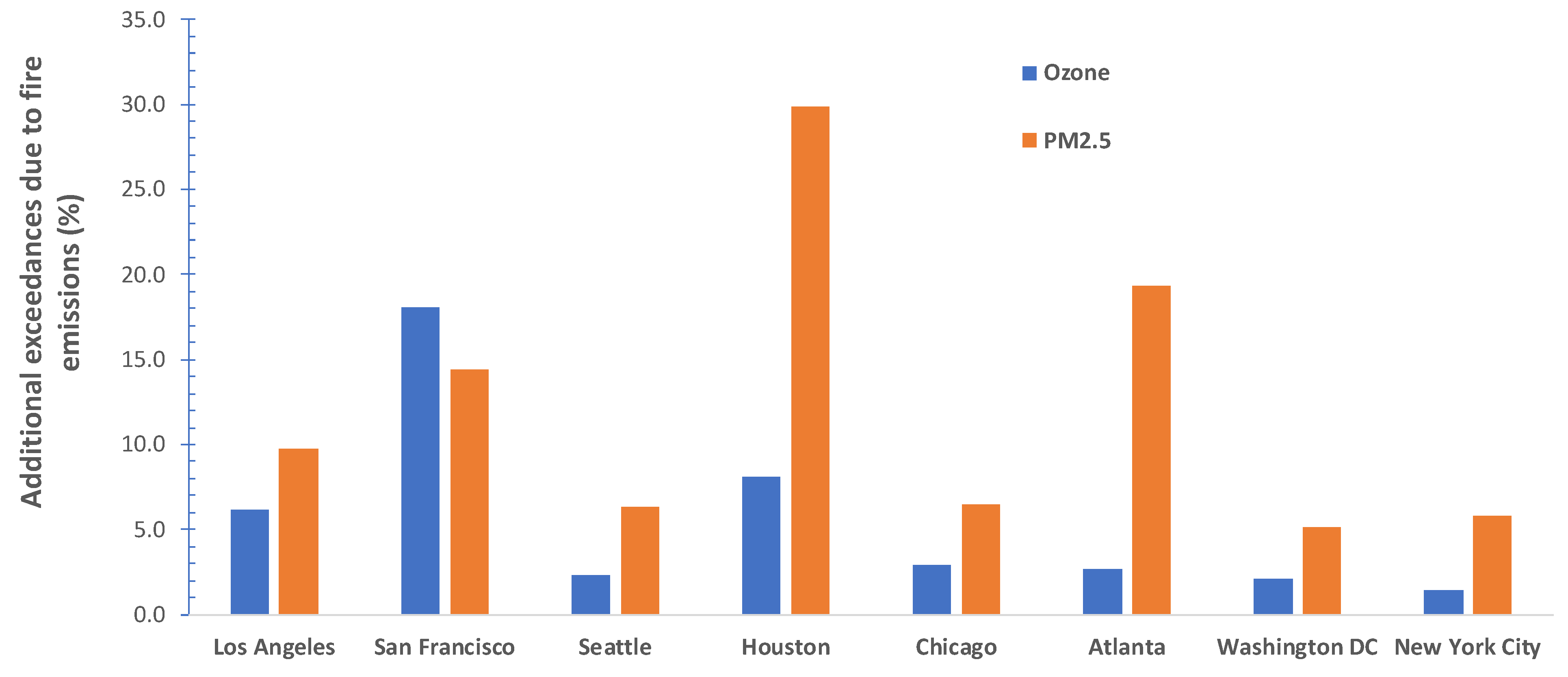
It was interesting to examine the effect of fire emissions on air quality over the metropolitan areas where a large population lives. Figure 9 illustrates the changes of surface O3 and PM2.5 exceedances due to the addition of fire emissions in the selected metropolitan areas from 1997 to 2016. It can be seen that except for San Francisco, fire generally caused higher percentage of more PM2.5 exceedances than that of O3. This was understandable since fire was the direct source of many PM2.5 components such as black carbon and organic carbon, whereas its impact on O3 was through emissions of its precursors such as CO and NOx in a complex nonlinear system. Fires led to 5.2% (Washington D.C.) ~ 29.9% (Houston) more PM2.5 exceedances while 1.5% (New York City) ~ 18.1% (San Francisco) more O3 exceedances. Moreover, it was not surprising that fire emissions affected air quality more in areas close to fire sources, e.g., San Francisco, Los Angeles, Houston, and Atlanta. However, fire emissions can cause extra exceedances over regions not often threatened by fires, e.g., Washington D.C. and New York City. Seeing the large number of people live and work in those mega cities, fire-induced bad air quality and its associated health damage should be taken into account in the future environmental planning.
4. Discussion and Conclusions
Taking advantage of the satellite observations of fire activities from space over the past two decades (1997–2016), this study examined the contributions of fire emissions to regional air quality over CONUS using the state-of-the-art regional modeling system encompassing CWRF climate, CMAQ air quality, and SMOKE emission models. In comparison with the ground observations, CWRF reproduced precipitation well with the domain average biases of less than 0.3 mm day−1 across 4 seasons. It overestimated surface temperature, especially over the Great Plains and Midwest in summer, but underestimated it over the western U.S. inter-mountain regions in winter. The domain average biases for winter, spring, summer, and autumn were -0.06 K, 0.68 K, 1.62 K, and 0.92 K, respectively. Overall, CMAQ slightly overestimated surface O3 by approximately 4% but underestimated surface PM2.5 by around 10%, as compared with the AQS observations.
Fire emissions increased the domain-average 20-year mean surface pollutant concentration slightly. The impacts on primary pollutant such as CO were generally confined to the fire source areas but the effects on secondary pollutant like O3 spread much broadly. The inter-annual variations in fire emissions impact on air quality were large with the maximum effect occurring during fire events. Fire occasionally accounted for more than 100 ppbv of monthly mean surface CO and over 20 µg m−3 of monthly mean PM2.5 from 1997 to 2016 in the northwestern U.S. and Northern California, two regions susceptible to frequent fires. Fire emissions did pose air quality compliance implications. From 1997 to 2016, fire emissions increased surface O3 exceedances (over NAAQS) by 10% and PM2.5 exceedances by 33%. In large portions of Northern California, Idaho, Montana, Wyoming, and New Mexico, there would have been no O3 exceedance days should no fire occur, suggested by the model simulation. Meanwhile, the PM2.5 exceedance days in large areas of California, the northwestern states, and Florida were almost exclusively caused by the addition of fire emissions.
It should be noted that the results out of the current investigation bear uncertainties. Although the quantification of model uncertainty is beyond the scope of this study, several uncertainty sources and their potential impacts on the research results would be discussed. First, the base year (2014) anthropogenic emissions was derived from the NEI2011 instead of NEI2014. This was mainly due to the logistic issue. When the project was initiated, the NEI2014 was not available. Therefore, the NEI2011 based emission data used by NOAA NAQFC was the best choice and adopted by this study. However, the usage of the NAQFC emissions data was not expected to make a large difference in the results for two reasons. (1) The NAQFC team has updated the NEI2011 to reflect changes in major sources, such as using EPA’s Continuous Emissions Monitors (CEMs) to update NOx and SO2 emissions of electricity generation units (EGUs) from the base year (2011) to model year [48]; (2) The focus of this study was to investigate the effects of fire emissions on air quality through examining the difference between two experiments with and without fire emissions. Therefore, the uncertainty introduced by the anthropogenic emissions tended to cancel out each other from two experiments.
Second, the uncertainty in any fire emissions inventory is large. Large negative biases of surface PM2.5 simulation have been identified in Section 3.2 when compared to the AQS observations in the fire susceptible regions. As pointed out by Pan et al. [70], the GFEDv4s dataset used in this study bears the smallest fire emissions over the temperate North America that includes CONUS. Moreover, the potential misrepresentation of plume height might mistakenly allocate fire emission at the wrong altitude. This indicates that the contribution of fire emissions to air quality may be at the low end out of this study. Therefore, an ensemble approach that considers multiple fire emissions inventories including plume height information may assist in reducing uncertainty in air quality modeling in the future.
Last but not the least, it is a known issue that CMAQ bears large uncertainty in modeling the secondary organic aerosol (SOA). Recent implementation of the volatility basis set (VBS) in CMAQ (CMAQ-VBS) [71] has significantly improved SOA prediction. However, the SOA formation efficiency is still two times too low [72]. Recent lab study [73] shows that more than half of the biomass burning emitted non-methane VOC can be converted to SOA after 6 days. Therefore, the underestimate of SOA in CMAQ likely affects the predicted PM2.5 resulting from fire emissions, especially in the downwind regions.
Although it is typically not factored into the designation of air quality non-compliance areas, wildfire induced bad air quality cannot be ignored for its adverse health effects. Based on the projections by Spracklen et al. [18] and Hawbaker and Zhu [19], the U.S. wildfire activities would increase toward the middle of the 21st century. This indicates that, with the continuing effort of reducing anthropogenic emissions and the increasing likelihood of more fire incidents in the future, air quality managers must take fire into account when formulating strategies on air quality compliances and human health protection. In addition, according to the National Interagency Fire Center, the prescribed fires account for between 14% and 42% of the total burnt areas over U.S. from 1998 to 2016. The inter-annual variation is large, but the prescribed fire is an important source of emissions in the U.S. Therefore, besides taking necessary measures to mitigate impacts of wildfires, the environmental policy makers should also better manage the prescribed fires to minimize their impact on air quality.
Author Contributions
Conceptualization, Z.T. and X.-Z.L.; methodology, Z.T., H.H., and X.-Z.L.; software, Z.T., H.H., and C.S.; validation: H.H. and C.S.; formal analysis, Z.T. and H.H.; investigation, Z.T., H.H., and X.-Z.L.; resources, D.T., X.-Z.L., and Z.T.; data curation: D.T., H.H., and C.S.; writing—original draft preparation, Z.T.; writing—review and editing, Z.T., H.H., C.S., D.T., and X.-Z.L.; project administration, X.-Z.L. and Z.T.; funding acquisition, X.-Z.L. and Z.T. All authors have read and agreed to the published version of the manuscript.
Funding
This research was partially funded by U.S. Environmental Protection Agency Science to Achieve Results (RD83587601), U.S. National Science Foundation Innovations at the Nexus of Food, Energy and Water Systems (EAR-1639327), and National Aeronautics and Space Administration (NASA) Modeling, Analysis, and Prediction Program.
Acknowledgments
The model simulations and analyses were conducted on the supercomputers, including the University of Illinois’ Blue Water, the Computational and Information Systems Lab of the National Center for Atmospheric Research, the Maryland Advanced Research Computing Center’s Bluecrab, the National Energy Research Scientific Computing Center of U.S. Department of Energy, and the NASA Center for Climate Simulation. We thank Kenneth Kunkel for providing the Cooperative Observer network station data. The views expressed in this document are solely those of the authors and do not necessarily reflect those of the funding Agency.
Conflicts of Interest
The authors declare no conflict of interest. The funders had no role in the design of the study; in the collection, analyses, or interpretation of data; in the writing of the manuscript, or in the decision to publish the results.
References
- Westerling, A.L.; Hidalgo, H.G.; Cayan, D.R.; Swetnam, T.W. Warming and earlier spring increase western, U.S. forest wildfire activity. Science 2006, 313, 940–943. [Google Scholar] [CrossRef] [Green Version]
- Rogers, B.M.; Neilson, R.P.; Drapek, R.; Lenihan, J.M.; Wells, J.R.; Bachelet, D.; Law, B.E. Impacts of climate change on fire regimes and carbon stocks of the U.S. Pacific Northwest. J. Geophys. Res. Biogeosci. 2011, 116, G03037. [Google Scholar] [CrossRef] [Green Version]
- Delfino, R.J.; Brummel, S.; Wu, J.; Stern, H.; Ostro, B.; Lipsett, M.; Winer, A.; Street, D.H.; Zhang, L.; Tjoa, T.; et al. The relationship of respiratory and cardiovascular hospital admissions to the southern California wildfires of 2003. Occup. Environ. Med. 2009, 66, 189–197. [Google Scholar] [CrossRef] [Green Version]
- Kochi, I.; Donovan, G.H.; Champ, P.A.; Loomis, J.B. The economic cost of adverse health effects from wildfire-smoke exposure: A review. Int. J. Wildland Fire 2010, 19, 803–817. [Google Scholar] [CrossRef]
- Haikerwal, A.; Akram, M.; Del Monaco, A.; Smith, K.; Sim, M.R.; Meyer, M.; Tonkin, A.M.; Abramson, M.J.; Dennekamp, M. Impact of fine particulate matter (PM2.5) exposure during wildfires on cardiovascular health outcomes. J. Am. Heart Assoc. 2015, 4, e001653. [Google Scholar] [CrossRef] [Green Version]
- Liu, J.C.; Pereira, G.; Uhl, S.A.; Bravo, M.A.; Bell, M.L. A systematic review of the physical health impacts from non-occupational exposure to wildfire smoke. Environ. Res. 2015, 136, 120–132. [Google Scholar] [CrossRef] [Green Version]
- Colarco, P.R.; Schoeberl, M.R.; Doddridge, B.G.; Marufu, L.T.; Torres, O.; Welton, E.J. Transport of smoke from Canadian forest fires to the surface near Washington, DC: Injection height, entrainment, and optical properties. J. Geophys. Res. Atmos. 2004, 109, D06203. [Google Scholar] [CrossRef]
- DeBell, L.J.; Talbot, R.W.; Dibb, J.E.; Munger, J.W.; Fischer, E.V.; Frolking, S.E. A major regional air pollution event in the northeastern United States caused by extensive forest fires in Quebec, Canada. J. Geophys. Res. Atmos. 2004, 109, D19305. [Google Scholar] [CrossRef] [Green Version]
- Sapkota, A.; Symons, J.M.; Kleissl, J.; Wang, L.; Parlange, M.B.; Ondov, J.; Breysse, P.N.; Diette, G.B.; Eggleston, P.A.; Buckley, T.J. Impact of the 2002 Canadian forest fires on particulate matter air quality in Baltimore City. Environ. Sci. Technol. 2005, 39, 24–32. [Google Scholar] [CrossRef] [PubMed] [Green Version]
- Mathur, R. Estimating the impact of the 2004 Alaskan forest fires on episodic particulate matter pollution over the eastern United States through assimilation of satellite-derived aerosol optical depths in a regional air quality model. J. Geophys. Res. Atmos. 2008, 113, D17302. [Google Scholar] [CrossRef] [Green Version]
- Dreessen, J.; Sullivan, J.; Delgado, R. Observations and impacts of transported Canadian wildfire smoke on ozone and aerosol air quality in the Maryland region on 9–12 June 2015. J. Air Waste Manag. Assoc. 2016, 66, 842–862. [Google Scholar] [CrossRef] [PubMed]
- Jaffe, D.; Bertschi, I.; Jaegle, L.; Novelli, P.; Reid, J.S.; Tanimoto, H.; Vingarzan, R.; Westphal, D.L. Long-range transport of Siberian biomass burning emissions and impact on surface ozone in western North America. Geophys. Res. Lett. 2004, 31, L16106. [Google Scholar] [CrossRef] [Green Version]
- Junquera, V.; Russell, M.M.; Vizuete, W.; Kimura, Y.; Allen, D. Wildfires in eastern Texas in August and September 2000: Emissions, aircraft measurements, and impact on photochemistry. Atmos. Environ. 2005, 39, 4983–4996. [Google Scholar] [CrossRef]
- Jaffe, D.A.; Wigder, N.L. Ozone production from wildfires: A critical review. Atmos. Environ. 2012, 51, 1–10. [Google Scholar] [CrossRef]
- Singh, H.B.; Cai, C.; Kaduwela, A.; Weinheimer, A.; Wisthaler, A. Interactions of fire emissions and urban pollution over California: Ozone formation and air quality simulations. Atmos. Environ. 2012, 56, 45–51. [Google Scholar] [CrossRef]
- Jaffe, D.A.; Wigder, N.; Downey, N.; Pfister, G.; Boynard, A.; Reid, S.B. Impact of wildfires on ozone exceptional events in the western US. Environ. Sci. Technol. 2013, 47, 11065–11072. [Google Scholar] [CrossRef]
- Lu, X.; Zhang, L.; Yue, X.; Zhang, J.C.; Jaffe, D.A.; Stohl, A.; Zhao, Y.H.; Shao, J.Y. Wildfire influences on the variability and trend of summer surface ozone in the mountainous western United States. Atmos. Chem. Phys. 2016, 16, 14687–14702. [Google Scholar] [CrossRef] [Green Version]
- Spracklen, D.V.; Mickley, L.J.; Logan, J.A.; Hudman, R.C.; Yevich, R.; Flannigan, M.D.; Westerling, A.L. Impacts of climate change from 2000 to 2050 on wildfire activity and carbonaceous aerosol concentrations in the western United States. J. Geophys. Res. Atmos. 2009, 114, D20301. [Google Scholar] [CrossRef]
- Hawbaker, T.J.; Zhu, Z. Projected Future Wildland Fires and Emissions for the Western United States, Chapter 8 of Baseline and Projected Future Carbon Storage and Greenhouse-Gas Fluxes in Ecosystems of the Western United States. US Geological Survey Professional Paper 1797. 2012. Available online: https://pubs.usgs.gov/pp/1797/pdf/pp1797_Chapter8.pdf (accessed on 7 March 2020).
- Jacob, D.J.; Winner, D.A. Effect of climate change on air quality. Atmos. Environ. 2009, 43, 51–63. [Google Scholar] [CrossRef] [Green Version]
- Charlson, R.J.; Schwartz, S.E.; Hales, J.M.; Cess, R.D.; Coakley, J.A.J.; Hansen, J.E.; Hofmann, D.J. Climate forcing by anthropogenic aerosols. Science 1992, 255, 423–430. [Google Scholar] [CrossRef]
- Ramanathan, V.; Chung, C.; Kim, D.; Bettge, T.; Buja, L.; Kielh, J.T.; Washington, W.M.; Fu, Q.; Sikka, D.R.; Wild, M. Atmospheric brown clouds: Impacts on South Asian climate and hydrological cycle. Proc. Natl. Acad. Sci. USA 2005, 102, 5326–5333. [Google Scholar] [CrossRef] [PubMed] [Green Version]
- Bond, T.C.; Doherty, S.J.; Fahey, D.W.; Forster, P.M.; Berntsen, T.; DeAngelo, B.J.; Flanner, M.G.; Ghan, S.; Karcher, B.; Koch, D.; et al. Bounding the role of black carbon in the climate system: A scientific assessment. J. Geophys. Res. Atmos. 2013, 118, 5380–5552. [Google Scholar] [CrossRef]
- Creamean, J.M.; Suski, K.J.; Rosenfeld, D.; Cazorla, A.; DeMott, P.J.; Sullivan, R.C.; White, A.B.; Ralph, F.M.; Minnis, P.; Comstock, J.M.; et al. Dust and biological aerosols from the Sahara and Asia influence precipitation in the western U.S. Science 2013, 339, 1572–1578. [Google Scholar] [CrossRef] [PubMed] [Green Version]
- Tao, Z.; Yu, H.; Chin, M. The role of aerosol-cloud-radiation interactions in regional air quality—A NU-WRF study over the United States. Atmosphere 2015, 6, 1045–1068. [Google Scholar] [CrossRef] [Green Version]
- Tao, Z.; Yu, H.; Chin, M. Impact of transpacific aerosol on air quality over the United States: A perspective from aerosol-cloud-radiation interactions. Atmos. Environ. 2016, 125, 48–60. [Google Scholar] [CrossRef]
- Mueller, S.F.; Mallard, J.W. Contributions of natural emissions to ozone and PM2.5 as simulated by the Community Multiscale Air Quality (CMAQ) model. Environ. Sci. Technol. 2011, 45, 4817–4823. [Google Scholar] [CrossRef]
- Yang, E.S.; Christopher, S.A.; Kondragunta, S.; Zhang, X.Y. Use of hourly Geostationary Operational Environmental Satellite (GOES) fire emissions in a Community Multiscale Air Quality (CMAQ) model for improving surface particulate matter predictions. J. Geophys. Res. Atmos. 2011, 116, D04303. [Google Scholar] [CrossRef] [Green Version]
- Garcia-Menendez, F.; Hu, Y.T.; Odman, M.T. Simulating smoke transport from wildland fires with a regional-scale air quality model: Sensitivity to spatiotemporal allocation of fire emissions. Sci. Total Environ. 2014, 493, 544–553. [Google Scholar] [CrossRef]
- Herron-Thorpe, F.L.; Mount, G.H.; Emmons, L.K.; Lamb, B.K.; Jaffe, D.A.; Wigder, N.L.; Chung, S.H.; Zhang, R.; Woelfle, M.D.; Vaughan, J.K. Air quality simulations of wildfires in the Pacific Northwest evaluated with surface and satellite observations during the summers of 2007 and 2008. Atmos. Chem. Phys. 2014, 14, 12533–12551. [Google Scholar] [CrossRef] [Green Version]
- Skamarock, W.C.; Klemp, J.B.; Dudhia, J.; Gill, D.O.; Barker, D.M.; Duda, M.G.; Huang, X.-Y.; Wang, W.; Powers, J.G. A description of the advanced research WRF version 3. NCAR Technical Note, NCAR/TN-475+STR. In Citeseer; NCAR: Boulder, CO, USA, 2008; p. 113. [Google Scholar]
- Liang, X.-Z.; Xu, M.; Yuan, X.; Ling, T.; Choi, H.I.; Zhang, F.; Chen, L.; Liu, S.; Su, S.; Qiao, F.; et al. Regional climate-weather research and forecasting model. Bull. Am. Meteorol. Soc. 2012, 93, 1363–1387. [Google Scholar] [CrossRef]
- Ling, T.-J.; Xu, M.; Liang, X.-Z.; Wang, J.X.L.; Noh, Y. A multi-level ocean mixed layer model resolving the diurnal cycle: Development and validation. J. Adv. Model. Earth Syst. 2015, 7, 1680–1692. [Google Scholar] [CrossRef] [Green Version]
- Yuan, X.; Liang, X.-Z. Improving cold season precipitation prediction by the nested CWRF-CFS system. Geophys. Res. Lett. 2011, 38, L02706. [Google Scholar] [CrossRef]
- Qiao, F.; Liang, X.-Z. Effects of cumulus parameterizations on predictions of summer flood in the Central United States. Clim. Dyn. 2015, 45, 727–744. [Google Scholar] [CrossRef]
- Qiao, F.; Liang, X.-Z. Effects of cumulus parameterization closures on simulations of summer precipitation over the United States coastal oceans. J. Adv. Model. Earth Syst. 2016, 8, 764–785. [Google Scholar] [CrossRef]
- Qiao, F.; Liang, X.-Z. Effects of cumulus parameterization closures on simulations of summer precipitation over the continental United States. Clim. Dyn. 2017, 49, 225–247. [Google Scholar] [CrossRef]
- Chen, L.-G.; Liang, X.-Z.; DeWitt, D.; Samel, A.N.; Wang, J.X.L. Simulation of seasonal US precipitation and temperature by the nested CWRF-ECHAM system. Clim. Dyn. 2016, 46, 879–896. [Google Scholar] [CrossRef]
- Liu, S.-Y.; Wang, J.; Liang, X.-Z.; Morris, V. A hybrid approach to improving the skills of seasonal climate outlook at the regional scale. Clim. Dyn. 2016, 46, 483–494. [Google Scholar] [CrossRef]
- Houyoux, M.R.; Vukovich, J.M.; Coats, C.J.J.; Wheeler, N.J.M. Emission inventory development and processing for the seasonal model for regional air quality (SMRAQ) project. J. Geophys. Res. 2000, 105, 9079–9090. [Google Scholar] [CrossRef]
- Briggs, G.A. Chimney plumes in neutral and stable surroundings (Discussion). Atmos. Environ. 1972, 6, 507–510. [Google Scholar] [CrossRef]
- EPA. CMAQ (Version 5.2) Scientific Document. Zenodo 2017, 234. [Google Scholar] [CrossRef]
- Otte, T.L.; Pleim, J.E. The meterology-chemistry interface preocessor (MCIP) for the CMAQ modeling system: Updates through MCIPv3.4.1. Geosci. Model Dev. 2010, 3, 243–256. [Google Scholar] [CrossRef] [Green Version]
- Chai, T.; Kim, H.; Lee, P.; Tong, D.; Pan, L.; Tang, Y.; Huang, J.; McQueen, J.; Tsidulko, M.; Stajner, I. Evaluation of the United States National Air Quality Forecast Capability experimental real-time predictions in 2010 using Air Quality System ozone and NO2 measurements. Geosci. Model Dev. 2013, 6, 1831–1850. [Google Scholar] [CrossRef] [Green Version]
- Huang, J.; McQueen, J.; Wilczak, J.; Djalalova, I.; Stajner, I.; Shafran, P.; Allured, D.; Lee, P.; Pan, L.; Tong, D.; et al. Improving NOAA NAQFC PM2.5 predictions with a bias correction approach. Weather Forecast. 2017, 32, 407–421. [Google Scholar] [CrossRef]
- Lee, P.; McQueen, J.; Stajner, I.; Huang, J.; Pan, L.; Tong, D.; Kim, H.; Tang, Y.; Kondragunta, S.; Ruminski, M.; et al. NAQFC developmental forecast guidance for fine particulate matter (PM2.5). Weather Forecast. 2017, 32, 343–360. [Google Scholar] [CrossRef]
- Pan, L.; Kim, H.C.; Lee, P.; Saylor, R.; Tang, Y.; Tong, D.; Baker, B.; Kondragunta, S.; Xu, C.; Ruminski, M.G.; et al. Evaluating a fire smoke simulation algorithm in the National Air Quality Forecast Capability (NAQFC) by using multiple observation data sets during the Southeast Nexus (SENEX) field campaign. Geosci. Model Dev. Discuss. 2018. [Google Scholar] [CrossRef] [Green Version]
- Tong, D.Q.; Lamsal, L.; Pan, L.; Ding, C.; Kim, H.; Lee, P.; Chai, T.-F.; Pickering, K.E.; Stajner, I. Long-term NOx trends over large cities in the United States during the great recession: Comparison of satellite retrievals, ground observations, and emission inventories. Atmos. Environ. 2015, 107, 70–84. [Google Scholar] [CrossRef]
- Randerson, J.T.; Van Der Werf, G.R.; Giglio, L.; Collatz, G.J.; Kasibhatla, P.S. Global Fire Emissions Database, Version 4.1 (GFEDv4); ORNL Distributed Active Archive Center: Oak Ridge, TN, USA, 2017. [Google Scholar] [CrossRef]
- Van der Werf, G.R.; Randerson, J.T.; Giglio, L.; van Leeuwen, T.T.; Chen, Y.; Rogers, B.M.; Mu, M.Q.; van Marle, M.J.E.; Morton, D.C.; Collatz, G.J.; et al. Global fire emissions estimates during 1997–2016. Earth Syst. Sci. Data 2017, 9, 697–720. [Google Scholar] [CrossRef] [Green Version]
- Liang, X.-Z.; Sun, C.; Zheng, X.; Dai, Y.; Xu, M.; Choi, H.I.; Ling, T.-J.; Qiao, F.; Kong, X.; Bi, X.; et al. CWRF performance at downscaling China climate characteristics. Clim. Dyn. 2019, 52, 2159–2184. [Google Scholar] [CrossRef]
- Chou, M.-D.; Suarez, M.J. A Solar Radiation Parameterization for Atmospheric Studies. [Last Revision on March 2002]. In Technical Report Series on Global Modeling and Data Assimilation; Suarez, M.J., Ed.; Goddard Space Flight Center: Greenbelt, MD, USA, 1999; Volume 15, p. 42. [Google Scholar]
- Chou, M.-D.; Suarez, M.J.; Liang, X.-Z.; Yan, M.M.-H.; Cote, C. A thermal infrared radiation parameterization for atmospheric studies. NASA Tech. Mem. 2001, 19, 56. [Google Scholar]
- Tao, W.-K.; Simpson, J.; Baker, D.; Braun, S.; Chou, M.-D.; Ferrier, B.; Johnson, D.; Khain, A.; Lang, S.; Lynn, B.; et al. Microphysics, radiation and surface processes in the Goddard Cumulus Ensemble (GCE) model. Meteorol. Atmos. Phys. 2003, 82, 97–137. [Google Scholar] [CrossRef]
- Holtslag, A.A.M.; Boville, B.A. Local Versus Nonlocal Boundary-Layer Diffusion in a Global Climate Model. J. Clim. 1993, 6, 1825–1842. [Google Scholar] [CrossRef] [Green Version]
- Liang, X.-Z.; Choi, H.; Kunkel, K.E.; Dai, Y.; Joseph, E.; Wang, J.X.L.; Kumar, P. Surface boundary conditions for mesoscale regional climate models. Earth Interact. 2005, 9, 1–28. [Google Scholar] [CrossRef]
- Liang, X.-Z.; Xu, M.; Gao, W.; Kunkel, K.E.; Slusser, J.; Dai, Y.; Min, Q.; Houser, P.R.; Rodell, M.; Schaaf, C.B.; et al. Development of land surface albedo parameterization bases on Moderate Resolution Imaging Spectroradiometer (MODIS) data. J. Geophys. Res. 2005, 110, D11107. [Google Scholar] [CrossRef] [Green Version]
- Choi, H.I.; Kumar, P.; Liang, X.-Z. Three-dimensional volume-averaged soil moisture transport model with a scalable parameterization of subgrid topographic variability. Water Resour. Res. 2007, 43, 15. [Google Scholar] [CrossRef] [Green Version]
- Choi, H.I.; Liang, X.-Z. Improved Terrestrial Hydrologic Representation in Mesoscale Land Surface Models. J. Hydrometeorol. 2010, 11, 797–809. [Google Scholar] [CrossRef]
- Yuan, X.; Liang, X.-Z. Evaluation of a Conjunctive Surface-Subsurface Process model (CCSP) over the contiguous United States at regional–local scales. J. Hydrometeorol. 2011, 12, 579–599. [Google Scholar] [CrossRef]
- Choi, H.I.; Liang, X.-Z.; Kumar, P. A conjunctive surface-subsurface flow representation for mesoscale land surface models. J. Hydrometeorol. 2013, 14, 1421–1442. [Google Scholar] [CrossRef]
- Xu, M.; Liang, X.-Z.; Samel, A.; Gao, W. MODIS consistent vegetation parameter specifications and their impacts on regional climate simulations. J. Clim. 2014, 27, 8578–8596. [Google Scholar] [CrossRef]
- Dee, D.P.; Uppala, S.M.; Simmons, A.J.; Berrisford, P.; Poli, P.; Kobayashi, S.; Andrae, U.; Balmaseda, M.A.; Balsamo, G.; Bauer, P.; et al. The ERA-Interim reanalysis: Configuration and performance of the data assimilation system. Quar. J. R. Meteorol. Soc. 2011, 137, 553–597. [Google Scholar] [CrossRef]
- Durre, I.; Menne, M.J.; Gleason, B.E.; Houston, T.G.; Vose, R.S. Comprehensive automated quality assurance of daily surface observations. J. Appl. Meteor. Clim. 2010, 49, 1615–1633. [Google Scholar] [CrossRef] [Green Version]
- Menne, M.J.; Durre, I.; Vose, R.S.; Gleason, B.E.; Houston, T.G. An overview of the global historical climatology network-daily database. J. Atmos. Ocean. Tech. 2012, 29, 897–910. [Google Scholar] [CrossRef]
- Daly, C.; Neilson, R.P.; Phillips, D.L. A Statistical-topographic model for mapping climatological preicipitation over mountainous terrain. J. Appl. Meteorol. 1994, 33, 140–158. [Google Scholar] [CrossRef] [Green Version]
- Liang, X.-Z.; Li, L.; Kunkel, K.E. Regional climate model simulation of U.S. precipitation during 1982-2002. Part I: Annual cycle. J. Clim. 2004, 17, 3510–3529. [Google Scholar] [CrossRef]
- Cressman, G. An operational objective analysis system. Mon. Weather Rev. 1959, 87, 367–374. [Google Scholar] [CrossRef]
- He, H.; Liang, X.-Z.; Sun, C.; Tao, Z.; Tong, D.Q. The long-term trend and production sensitivity change of the U.S. ozone pollution from observations and model simulations. Atmos. Chem. Phys. Discuss. 2019. [Google Scholar] [CrossRef]
- Pan, X.; Ichoku, C.; Chin, M.; Bian, H.; Darmenov, A.; Colarco, P.; Ellison, L.; Kucsera, T.; da Silva, A.; Wang, J.; et al. Six global biomass burning emissions datasets: Intercomparison and application in one global aerosol model. Atmos. Chem. Phys. 2020, 20, 969–994. [Google Scholar] [CrossRef] [Green Version]
- Donahue, N.; Chuang, W.; Epstein, S.; Kroll, J.; Worsnop, D.; Robinson, A.; Adams, P.; and Pandis, S. Why do organic aerosols exist? Understanding aerosol lifetimes using the two- dimensional volatility basis set. Environ. Chem. 2013, 10, 151–157. [Google Scholar] [CrossRef] [Green Version]
- Woody, M.; Baker, K.; Hayes, P.; Jimenez, J.; Koo, B.; Pye, H. Understanding sources of organic aerosol during CalNex-2010 using the CMAQ-VBS. Atmos. Chem. Phys. 2016, 16, 4081–4100. [Google Scholar] [CrossRef] [Green Version]
- Lim, C.Y.; Hagan, D.H.; Coggon, M.M.; Koss, A.R.; Sekimoto, K.; de Gouw, J.; Warneke, C.; Cappa, C.D.; Kroll, J.H. Secondary organic aerosol formation from the laboratory oxidation of biomass burning emissions. Atmos. Chem. Phys. 2019, 19, 12797–12809. [Google Scholar] [CrossRef] [Green Version]
Figure 1.
(a) Evolution of fire emissions from 1997 to 2016 normalized to the 2014 levels. Numbers are 2014 emissions in metric tons for each species. (b) Variations in ratios of fire to anthropogenic emissions from 1997 to 2016 for selected species, right y-axis is for OC only.
Figure 1.
(a) Evolution of fire emissions from 1997 to 2016 normalized to the 2014 levels. Numbers are 2014 emissions in metric tons for each species. (b) Variations in ratios of fire to anthropogenic emissions from 1997 to 2016 for selected species, right y-axis is for OC only.

Figure 2.
Spatial distributions of fire CO emissions (tons km−2 yr−1) for 1998, 2002, 2013, and 2015. Boxes over the maps represent the sub-regions subject to further analysis–southeastern U.S.; Northern California, and northwestern U.S.
Figure 2.
Spatial distributions of fire CO emissions (tons km−2 yr−1) for 1998, 2002, 2013, and 2015. Boxes over the maps represent the sub-regions subject to further analysis–southeastern U.S.; Northern California, and northwestern U.S.

Figure 3.
Differences (modeled–observed) of 20-year average T2 (top) and precipitation (bottom) over the contiguous U.S. for winter (DJF), spring (MAM), summer (JJA), and fall (SON). Numbers in brown, blue, and red represent the bias, correlation coefficient, and root mean square error (RMSE), respectively.

Figure 4.
Comparisons of annual-mean surface O3 (left) and PM2.5 (right) between community multiscale air quality (CMAQ) modeled results and air quality system (AQS) observations over the years of 2000-2016. Each point represents a paired simulated and measured data in time and space. The color bar shows the scatter density (%) of measured vs. modeled O3 (left, in 1 ppbv bin) and PM2.5 (right, in 0.4 µg m−3 bin).

Figure 5.
Top panels: spatial distribution of fire contributions to 20-year average surface air quality of CO (ppbv), O3 (ppbv), and PM2.5 (µg m−3); bottom panels: evolutions of annual average surface concentrations of CO, O3, and PM2.5 from 1997–2016.
Figure 5.
Top panels: spatial distribution of fire contributions to 20-year average surface air quality of CO (ppbv), O3 (ppbv), and PM2.5 (µg m−3); bottom panels: evolutions of annual average surface concentrations of CO, O3, and PM2.5 from 1997–2016.

Figure 6.
Evolutions of fire contributions to monthly average surface CO (ppbv), O3 (ppbv), and PM2.5 (µg m−3) for the northwestern U.S., Northern California, and the southeastern U.S. from 1997 to 2016.
Figure 6.
Evolutions of fire contributions to monthly average surface CO (ppbv), O3 (ppbv), and PM2.5 (µg m−3) for the northwestern U.S., Northern California, and the southeastern U.S. from 1997 to 2016.

Figure 7.
Probability distribution of surface 8-hr average O3 (top) and 24-hr average PM2.5 (bottom) concentrations over the contiguous U.S. The inlet on each plot is the re-normalized probability distribution of the corresponding pollutant at tail with high concentrations.
Figure 7.
Probability distribution of surface 8-hr average O3 (top) and 24-hr average PM2.5 (bottom) concentrations over the contiguous U.S. The inlet on each plot is the re-normalized probability distribution of the corresponding pollutant at tail with high concentrations.

Figure 8.
Spatial distributions of extra air quality exceedance days due to addition of fire emissions over the years of 1997-2016 (left), and percentage contribution of fire emissions to 20-year total air quality exceedance days (, right).
Figure 8.
Spatial distributions of extra air quality exceedance days due to addition of fire emissions over the years of 1997-2016 (left), and percentage contribution of fire emissions to 20-year total air quality exceedance days (, right).

Figure 9.
Percentage changes in surface O3 and PM2.5 exceedances due to the addition of fire emissions in the selected metropolitan areas over 1997-2016.
Figure 9.
Percentage changes in surface O3 and PM2.5 exceedances due to the addition of fire emissions in the selected metropolitan areas over 1997-2016.

© 2020 by the authors. Licensee MDPI, Basel, Switzerland. This article is an open access article distributed under the terms and conditions of the Creative Commons Attribution (CC BY) license (http://creativecommons.org/licenses/by/4.0/).
Share and Cite
MDPI and ACS Style
Tao, Z.; He, H.; Sun, C.; Tong, D.; Liang, X.-Z. Impact of Fire Emissions on U.S. Air Quality from 1997 to 2016–A Modeling Study in the Satellite Era. Remote Sens. 2020, 12, 913. https://doi.org/10.3390/rs12060913
AMA Style
Tao Z, He H, Sun C, Tong D, Liang X-Z. Impact of Fire Emissions on U.S. Air Quality from 1997 to 2016–A Modeling Study in the Satellite Era. Remote Sensing. 2020; 12(6):913. https://doi.org/10.3390/rs12060913
Chicago/Turabian StyleTao, Zhining, Hao He, Chao Sun, Daniel Tong, and Xin-Zhong Liang. 2020. "Impact of Fire Emissions on U.S. Air Quality from 1997 to 2016–A Modeling Study in the Satellite Era" Remote Sensing 12, no. 6: 913. https://doi.org/10.3390/rs12060913
Note that from the first issue of 2016, this journal uses article numbers instead of page numbers. See further details here.