Applying Satellite Data Assimilation to Wind Simulation of Coastal Wind Farms in Guangdong, China


1
Ministry of Education Key Laboratory for Earth System Modeling, Department of Earth System Science, Tsinghua University, Beijing 100084, China
2
Key Laboratory of Ecosystem Network Observation and Modeling, Institute of Geographic Sciences and Natural Resources Research, Chinese Academy of Sciences, Beijing 100101, China
3
Yucheng Comprehensive Experiment Station, Chinese Academy of Science, Beijing 100101, China
*
Author to whom correspondence should be addressed.
Remote Sens. 2020, 12(6), 973; https://doi.org/10.3390/rs12060973
Submission received: 19 February 2020
/
Revised: 13 March 2020
/
Accepted: 16 March 2020
/
Published: 17 March 2020
(This article belongs to the Special Issue Remote Sensing in Hydrology and Water Resources Management)
Abstract
:With the development of the wind power industry in China, accurate simulation of near-surface wind plays an important role in wind-resource assessment. Numerical weather prediction (NWP) models have been widely used to simulate the near-surface wind speed. By combining the Weather Research and Forecast (WRF) model with the Three-dimensional variation (3DVar) data assimilation system, our work applied satellite data assimilation to the wind resource assessment tasks of coastal wind farms in Guangdong, China. We compared the simulation results with wind speed observation data from seven wind observation towers in the Guangdong coastal area, and the results showed that satellite data assimilation with the WRF model can significantly reduce the root-mean-square error (RMSE) and improve the index of agreement (IA) and correlation coefficient (R). In different months and at different height layers (10, 50, and 70 m), the Root-Mean-Square Error (RMSE) can be reduced by a range of 0–0.8 m/s from 2.5–4 m/s of the original results, the IA can be increased by a range of 0–0.2 from 0.5–0.8 of the original results, and the R can be increased by a range of 0–0.3 from 0.2–0.7 of the original results. The results of the wind speed Weibull distribution show that, after data assimilation was used, the WRF model was able to simulate the distribution of wind speed more accurately. Based on the numerical simulation, our work proposes a combined wind resource evaluation approach of numerical modeling and data assimilation, which will benefit the wind power assessment of wind farms.

1. Introduction
Energy from fossil fuels has played a major role in the development of modern human civilization, but it also brings serious environmental problems and climate issues, such as atmospheric environmental pollution and global warming. The development of renewable energy is one of the major ways to solve environmental problems and achieve sustainable development; wind energy has been developed rapidly as the main clean and renewable energy.
In 2018, China installed an additional wind power capacity of 21 GW and thus has total wind power capacity of more than 200 GW [1]. Before the construction of wind farms, wind resources in wind farm areas need to be evaluated, and the location selection of a wind farm is mainly based on the results of the wind resource assessment. Therefore, wind speed simulation in the wind farm area is a key issue in the development of wind power.
After many years of development, wind speed simulation in wind resource assessment and prediction now has two methods: the statistical method and numerical simulation. Costa et al. [2] made a brief review about the development of the short-term wind speed forecast during 30 years of history, highlighting that the main forecast method has changed from the statistical model into the numerical model, and that the integration between both models has also begun to be used. Storm et al. [3] used the Weather Research and Forecast (WRF) [4] model to simulate the LLJ (low-level jet), and the model was able to capture some characteristics of LLJ, which indicates that WRF model can be used for short-term wind energy simulation.
In order to improve the accuracy of the numerical weather model in wind speed simulation, there are two approaches: (1) developing the physical parameterization scheme to improve the wind simulation performance at near-surface levels and (2) applying the data assimilation to improve the initial condition of the atmosphere. Some research studies evaluated the parameterization scheme chosen and planetary boundary layer (PBL) development [5,6,7,8]. In addition to the selection and improvement of the PBL scheme, data assimilation is also widely used to improve the wind simulation results of the numerical model.
Liu et al. [9] combined the WRF model with a data assimilation system and a large eddy simulation (LES) model, which increased wind energy simulation resolution to the level of LES. Zhang et al. [10] used the WRF model and data assimilation to forecast near-surface wind speed. In this work, the conventional observations and infrared satellite observations were used to improve the model output wind speed by the 3DVar. The results showed that, with the improvements of the initial fields, the assimilation of conventional observations and infrared satellite observations significantly improved the wind forecast results. Ancell et al. [11] compared the effects of the ensemble Kalman filter and 3Dvar data assimilation on wind forecasting. The results showed that the EnKF assimilation effect is better than the 3DVar assimilation for 24-h forecasting. Ulazia et al. [12] compared different data assimilation schemes and found that the assimilation at an interval of six hours has a better effect on the simulation of wind speed than at an interval of 12 h. The study also suggested applying data assimilation techniques to mesoscale weather models in wind resource assessment. Che et al. [13] developed a system to predict wind speed at turbine height. The Kalman filter algorithm was used to assimilate the cabin wind data after quality control, and the wind speed prediction of the WRF model was improved. The study also pointed out that data assimilation can effectively reduce random errors and is more important in rare or extreme weather conditions. Ulazia et al. [14] used the WRF model to estimate the offshore wind energy resources on the Iberian Mediterranean coast and the Balearic Islands. The results of data assimilation and no data assimilation were compared. The results showed that the bias of the wind speed simulation after the 3DVar data assimilation was significantly reduced. Cheng et al. [15] improved short-term (0–3 h) wind energy forecasting by assimilating wind speed observed in wind turbines into a numerical weather forecast system. The results showed that the assimilation of wind speed can reduce the average absolute error of the wind speed forecast for 0–3 h by 0.5–0.6 m/s.
As can be seen from related works, data assimilation can improve short-term wind speed simulation results by changing the initial field and providing real-time updates during the model run. An efficient way is dividing long-time simulation into multiple short-time simulations, using the previous numerical weather prediction (NWP) output as the “first guess” field, and then applying data assimilation to update the initial condition and to continue the next short-time run.
In this paper, we used the WRF (Weather Research and Forecast) model to make a one-year wind speed simulation on the coastal wind farm area in Yangjiang, Guangdong. Furthermore, the 3DVar data assimilation was used to assimilate the satellite radiation data. The observation data of seven wind observation towers were used to measure the simulation results and to calculate the improvements of data assimilation on near-surface wind speed simulation. The remainder of this paper is organized as follows: Section 2 mainly introduces the experiment, the data, and the results of the measurement methods; Section 3 analyzes the results of the different tests; Section 4 discusses the results of this article compared with other work; and Section 5 presents the main conclusions.
2. Materials and Methods
2.1. Wind Observation Data
In order to estimate the improvement of the satellite data assimilation to wind speed simulation, wind speed observations from seven wind observation towers were used. These wind towers have wind speed observations at different heights (10, 50, and 70 m) and measure the instantaneous wind speed and direction every 10 min. The data of wind towers were provided by China Huaneng Group Co., Ltd. (CHNG), and all wind towers are located in the wind farm of CHNG.
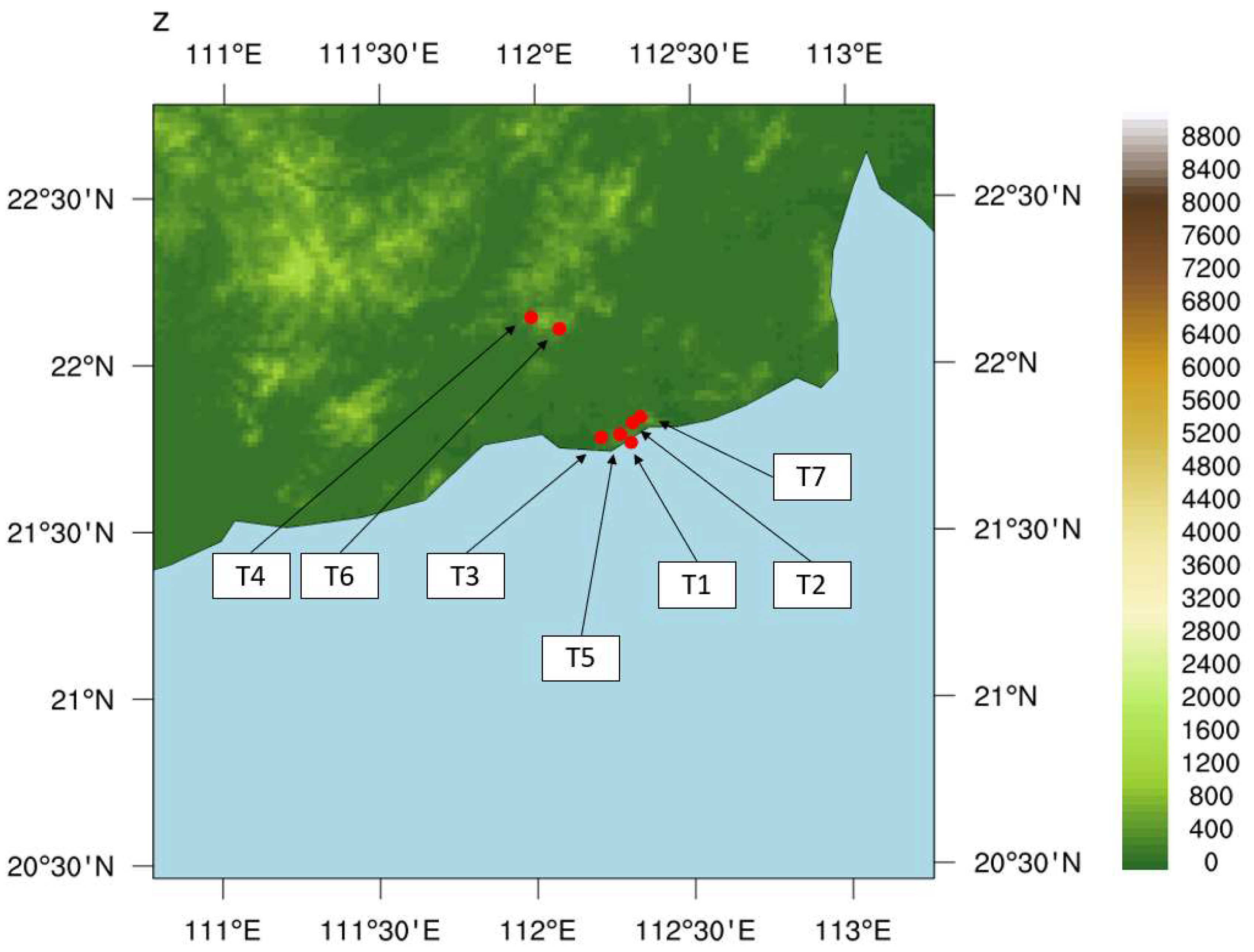
Table 1 shows the geographical locations and altitudes of the seven wind towers. These wind towers are geographically close, and all of them are located near the coastal area in Yangjiang, Guangdong Province. Table 2 is the wind-sensor type, model number, hardware, and software version of wind towers. Figure 1 shows these towers’ locations in the inner domain of the model.
The observation time of the wind towers is the whole year of 2012. For the original data, quality control (QC) was performed first; another wind resource assessment research study [16] used the similar type of wind observations, so we used the same QC method as that study. The QC method was as follows: (1) If the wind speed value does not change for more than 30 min, these data are regarded as invalid data. (2) If there is a large difference between the observed wind speeds at different heights, the data with small value at that time are also considered as invalid data. The comparison methods were as follows: , , or , where , , and are the wind speed at 70, 50, and 10 m.
Table 3 shows the observation data numbers of each wind tower in the different months of 2012, and Table 4 is the observation data amount after the quality control. Some towers have missing data in autumn and winter. The data of Tower 5 at heights of 50 and 70 m are considered invalid because of poor quality.
2.2. Numerical Model and Data Assimilation
We set three numerical simulation tests to measure the improvement of wind speed simulation by applying satellite data assimilation. The first test (Test 1) only used cold-start initial conditions from NCEP’s final analysis data to create a simulation of wind speed. The second test (Test 2) used the analysis field generated by the data assimilation system as the initial conditions, and the model field was updated four times by the data assimilation system during each simulation run. In order to compare the improvement of satellite data assimilation with conventional observations data, we set a third test (Test 3), which used the same data assimilation configurations of Test 2, except the conventional surface and upper-air observation data as the data assimilation input.
The Model we used in our work was the WRF model (version 3.8.1), and its data-assimilation system WRFDA [4] was used for satellite and conventional data assimilation. Figure 2 shows the three nested domains of our simulation tests. The inner domain we used in our simulations was mainly located in the coastal area of Yangjiang, Guangdong. Figure 1 shows the distribution of wind towers (red dots) in the inner domain. The chosen of physical configuration considered the following schemes: Morrison double-moment scheme [17] for microphysics; RRTMG [18] for longwave and shortwave radiation; Noah [19] for land-surface scheme; Kain–Fritsch [20] for cumulus convention; and YSU [21] for PBL. Table 5 shows the model configuration of simulations; since domain 03’s grid resolution was less than 5 km, we did not need to set the cumulus convention scheme for domain 03. All of the test cases (Test 1, Test 2, and Test 3) used the same WRF model configurations, including parameter settings and model domains. The ETA values of the near-surface layers were 1.0000, 0.9960, 0.9920, 0.9900, 0.9851… The average altitudes of near-surface layers in domain 03 were 16.31, 48.97, 73.52, and 101.85 m.
The data used to generate the initial condition and boundary forcing of the model were Final Operational Global Analysis Data (FNL) [22], which were provided by the National Centre for Environmental Prediction (NCEP). The spatial resolution of FNL data was 1 degree (both in latitude and longitude), and the temporal resolution was 6 h.
The background error covariance matrix used in 3DVar data assimilation was generated by the NMC method [23]. To calculate the background error, a one-month simulation was made from 1 Jan. 2012 to 1 Feb. 2012. The simulation had the same model settings as Test 1, 2, and 3, and it contained a 12-h forecast and 24-h forecast results at both 00:00 and 12:00 UTC. Then, the 62 pairs of results from the 31 days were used to calculate the background error covariance.
The NCEP GDAS Satellite Data [24] were used as the input data for satellite data assimilation. The satellite data sensors included AMSUA, HIRS, MHS, and AIRS. Table 6 shows the types of platforms and sensors. In order to process the satellite data before data assimilation, the Community Radiative Transfer Model (CRTM) was used as the radiative transfer model. The CRTM model can look up the Cloud coefficient, Surface Emissivity coefficient, and Aerosol coefficient and eliminate the satellite data bias caused by cloud, land, and aerosol. Table 7 shows the resolution of satellite data. Since some sensors (MHS, HIRS, and AIRS) have higher resolutions than domain 01 (27 km), we applied data-thinning to domain 01 in the data assimilation.
The conventional observations used in Test 3 includes NCEP ADP Global Surface Observational Weather Data [25] and NCEP ADP Global Upper Air Observational Weather Data [26]. Most of the conventional observations used in Test 3 are synoptic observations. Figure 3 shows the locations of synoptic observation stations.
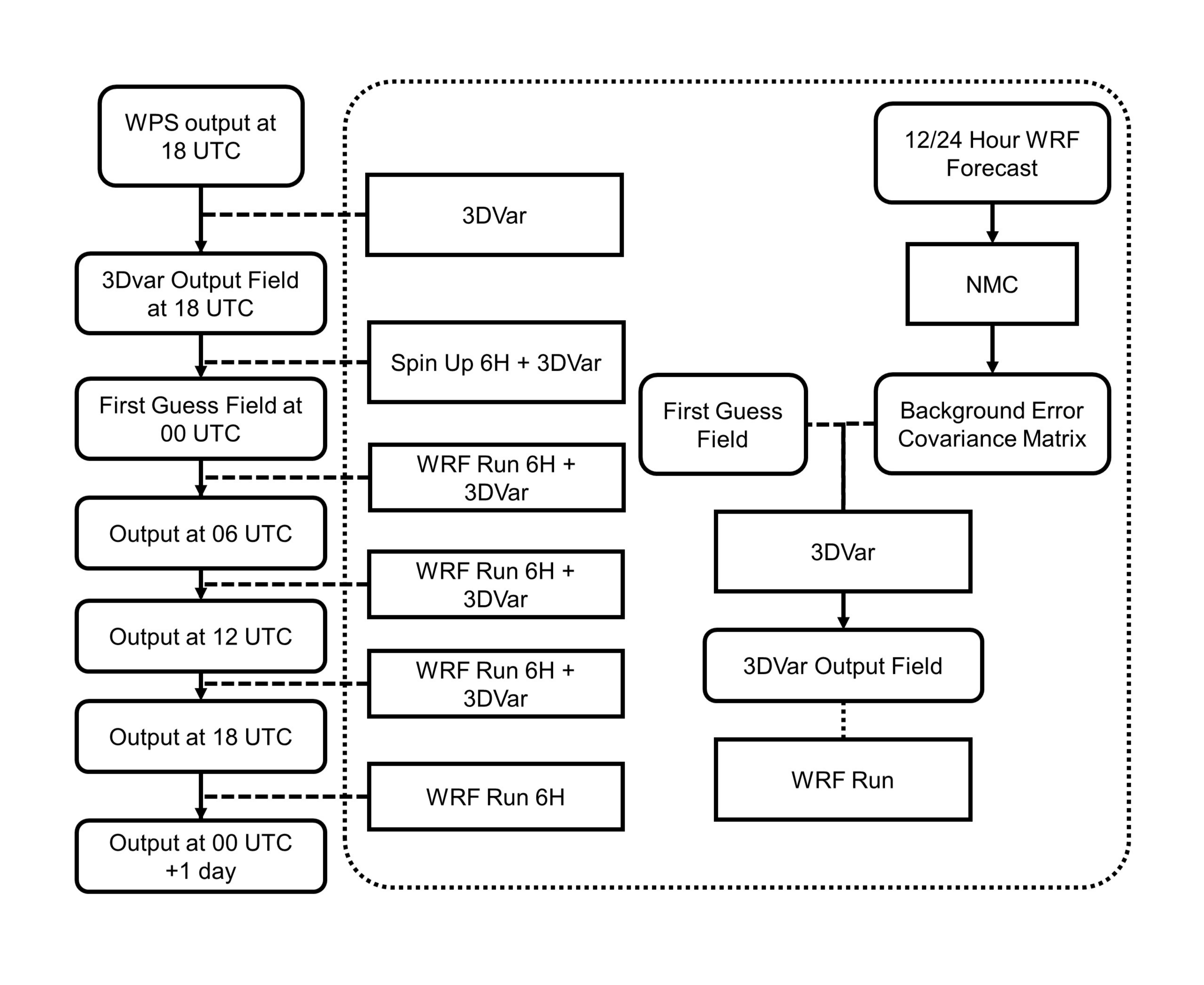
Figure 4 shows the method of the WRF run in the three tests. Because we needed to obtain values of wind speed every 10 min instead of long-term variability, we started the model every day in 2012, and each run of the model made just a one-day simulation. The reason for this was that long-time running depends on boundary forcing, which can capture long-term variability, but it cannot accurately simulate the results at every moment.
In Test 1, we started the WRF model at 18:00 UTC every day and took 6 h from 18:00 to 00:00 UTC as the spin-up time. Then, from 00:00 to 00:00 UTC the next day, the model output the simulated wind speed as the results of Test 1. Since the time interval of the observation data was 10 min, the time interval of the wind speed output of the model was also set to 10 min.
In Test 2 and Test 3, we used the WPS (WRF preprocessing system) output of 18:00 UTC as the first guess field, and then we assimilated the satellite observation data by using the 3DVar, and used the 3DVar output as the initial field of the WRF model. From 18:00 UTC to 00:00 UTC, the model was run as a spin up process. At 00:00 UTC (+1 day), 06:00 UTC (+1 day), 12:00 UTC (+1 day), and 18:00 UTC (+1 day), the data assimilation system was run four times, each time using the WRF output as the first guess field and the satellite data as the observation input.
Unlike the long-time cycling run of WRF-3Dvar, our model was cold-started daily based on FNL data. In Tests 1, 2, and 3, we used FNL data to generate the initial field, to run the WRF model for 30 h, and to begin the next day’s run. The only difference between Test 1 and Tests 2 and 3 was that Test 2 and Test 3 applied data assimilation five times in each WRF run. Another similar wind resource evaluation work [27] explained that this way avoids model divergence and the accumulation of truncation errors, and the WRF simulations used in that research were 2-day-restart runs. We also calculated the 3Dvar mean absolute difference (MAD) of U and V in domain 03 in Test 2, as follows:
Here, is the total grid number in domain 03; is the U or V wind speed after 3Dvar; and is the U or V wind speed of first guess field.
We calculated the MAD of U and V at 4 different 3Dvar times, in the simulation, including 00, 06, 12, and 18 UTC. The results of different height and different time MAD are shown in Figure 5; we can find that the MAD is stable at 00, 06, 12, and 18, so there is virtually no difference between the typical operational cycling run and our daily cold-start run.
After obtaining the model results, we first interpolated the three-dimensional wind field into heights of 10, 50, and 70 m, using linear interpolation. Then, we interpolated the wind field into the wind tower’s latitude and longitude, where the horizontal interpolation method was bilinear interpolation. We used the results of the interpolation to compare with the observed wind speed.
2.3. Results Measurements
In order to evaluate the results of the different tests, the following evaluation indices were calculated to evaluate the errors and correlations between model results and observation data.
2.3.1. Root-Mean-Square Error (RMSE)
The root-mean-square error (RMSE) is widely used in NWP to evaluate the error of wind speed and other meteorological variables. Since the observation data has a 10-minute time resolution, we used the 10-minute model output and calculated the RMSE of the 10-minute model wind speed output.
Here, is the number of wind speed observations in each month, is the value of the model result, and is the observation value.
2.3.2. Index of Agreement (IA)
Index of Agreement is a standardized measure of the degree of model prediction error [28,29,30]. It can be calculated by the following:
where is the average value of the total observation data.
The Index of Agreement varies between 0 and 1, where a value of IA close to 1 indicates well-matched results, and 0 indicates no agreement at all.
The index of agreement can detect additive and proportional differences in the observed and simulated means and variances [31]. We calculate the IA of the 10-minute model wind speed output to investigate the agreement level of the model output to the wind speed observations.
2.3.3. Pearson Correlation Coefficient (R)
The Pearson Correlation Coefficient (R) is also widely used to evaluate the performance of wind speed simulation of NWP. It reflects the correlation between wind speed simulation series and observation series. If the model output has a high level of R, the error can be largely corrected by postprocessing algorithms.
Here, represents the covariance of the model results and observation wind speed, and and represent the variance of the model results and observation wind speed. These variables can be calculated as follows:
In our tests, we calculate the R between the 10-minute model wind speed output and 10-minute wind speed observations. The R results were also compared, to evaluate the simulation results and the improvements of data assimilation.
2.3.4. Weibull Distribution of Wind Speed
In general, the distribution of near-surface wind speed can be fitted by Weibull distribution [32]. The probability density function of Weibull distribution is as follows:
where is the wind speed, is the shape parameter, and is the scale parameter of the Weibull distribution.
The Weibull distribution has been widely used in the wind resource assessment because, before the wind farm construction, the wind speed distribution must be evaluated in order to calculate the amount of electric power the wind farm can generate. The two parameters can be used to determine whether the distribution of wind speed simulation results is similar to the observations. If the parameters of wind simulation results are close to the observation, the distribution of model result can reflect the true wind distribution well, and the model results can be used in the wind resource assessment.
3. Results
3.1. The Wind Distribution Results
Figure 6 is the Weibull distribution of seven towers at 10, 50, and 70 m. Tower 5 was missing most of its data at 50 m and all its data at 70 m. Therefore, the distribution of Tower 5 at 50 and 70 m was not analyzed. Table 8 is the shape parameter and the scale parameter of each Weibull distribution in Figure 6. In all of the subfigures of Figure 6, we can see that the wind speed distribution of the red lines is generally smaller than the wind speed distribution of the green lines. This means that the wind speed of Test 2 is smaller than the wind speed of Test 1. Compared to the peak position of wind speed distribution and the peak value of the distribution, except in several cases (Tower 1 is 10 m; Tower 3 is 10 m; Tower 5 is 10 m; and Tower 6 is 10, 30, and 70 m), in most cases, the peak value of Test 2 is closer to the observation than Test 1. Furthermore, for the peak value of wind speed distribution, we can also find that, except in four cases (Tower 1 is 70 m, Tower 2 is 70 m, Tower 3 is 70 m, and Tower 6 is 70 m), the peak values of Test 2 are closer to the observations than Test 1. Table 8 shows that the shape and scale parameters of Test 1 are larger than those of Test 2 and Test 3; Test 1’s simulation performance is worse than Test 2’s and Test 3’s, mainly due to the systematic higher simulation of the wind speed.
3.2. The RMSE, IA, and R Results
The Table A1, Table A2 and Table A3 in Appendix A are the RMSE, IA, and R results of the three tests (Test 1, Test 2, and Test 3) at heights of 10, 50, and 70 m. In order to analyze the distributions in different months, the results of each wind tower were calculated separately in each month, from January to December. The vacant positions in the tables mean that there were no valid wind speed observations in that month, so indices were not calculated.
For the distributions of wind direction, we plot the wind rose in each month, using the wind speed and wind direction of Test 2. The Figure A1, Figure A2, Figure A3 and Figure A4 in Appendix B are the wind rose at different heights in the four seasons of spring, summer, autumn, and winter.
In the results of the correlation coefficients (R) in Table A1 and Table A2, Test 1 had two records that did not pass the significance test (10 m Tower 6 Jul. and 50 m Tower 5 Jan.). This is because (1) the amount of data was too small (790 and 63) and (2) the correlation coefficient was too small. The other correlation coefficients all passed the significance test, with more than 99% confidence.
After calculating the average value of the results for the different towers, we obtained the average distribution of RMSE, IA, and R. Figure 7 shows the seven towers’ average results of RMSE, IA, and R of Tests 1, 2, and 3, at 10, 50, and 70 m. As can be seen from Figure 7, the results of Test 2 and Test 3 are better than that of Test 1 on all three indices. Both conventional and satellite data can improve wind speed simulation. However, compared with Test 2, Test 3 has small improvements in RMSE, IA, and R. Compared with the conventional data, satellite data have a wider geographical coverage, and the improvement of wind speed simulation is more significant.
3.3. Wind Speed Simulation Results Analysis
From Table A1, Table A2 and Table A3, we can find that the RMSE of the model simulation results varied greatly in different months. In some towers, the gap between the different months even reached 2 m/s (10 m for Tower 2; 70 m for Tower 1) and, in most cases, there was at least a 0.5 m/s gap. Like RMSE, the R also changed greatly with the month. Furthermore, we also found that RMSE and R change a lot at different heights in some cases (Tower 2 December; Tower 3 December).
Stensrud et al. [33] compared the MM4 [34] model output with the observation temperature and found that there is systematic bias in the NWP model. In order to analyze the systematic bias, we calculated the mean wind speed value of Test 1, Test 2, and observation data in each month, and we obtained the wind speed anomalies by using the following equation:
where is the wind speed anomalies, and is the mean values of wind speed in each month.
In order to analyze the wind speed simulation results in Test 1 and to find out the performance of the WRF model on wind speed simulation, we calculated the RMSE, IA, and R by using the wind speed and wind speed anomalies of Test 1 and observations. Figure 8 shows the results of the average indices from seven towers. We also calculated the average value of the bias of mean speed of Test 1 and Test 2; the results are shown in Figure 9.
In Figure 8, we can find that, in the same month and at the same height, the IA is similar between wind speed and wind speed anomalies, but sometimes the value of RMSE can be very different. As for RMSE, the difference between wind speed and wind speed anomalies can be caused by systematic bias of the model’s simulations. Therefore, when the model has systematic bias, the RMSE gap will become larger. In some months with large RMSE values, the RMSE gap is always large, indicating that part of the error is caused by systematic bias.
In Figure 8, the RMSE is less than 3 m/s in May, June, July, August, and September, of which the lowest value is in August. Among the IA results, August still reaches the highest value, and the values of April and May are lower than the rest of the months. The results of R are similar to those of IA, having the highest value in August and the lowest values in April and May. From these distributions of the indices, the simulation results in summer are generally the best, and the simulation results in spring are the worst. From the Figure A1 in Appendix B, we can see that the main wind directions in spring are east, south, and southeast, and the wind speed distribution is particularly dense in some directions, namely from ocean to land. We can infer that the poor performance of the spring simulation may be caused by the wind from the ocean. However, in summer (Figure A2), especially in July and August, although there are winds in the ocean direction, the wind still distributes in many directions.
From the performance of RMSE, MAE, IA, and R in winter, we can see that, although the RMSE and MAE values are large in winter, IA and R are also large. From the RMSEs of wind speed and wind speed anomalies, we can find that the gap between them in winter is larger, when compared with other months. Figure 9 also shows that, in winter, the bias of mean speed is larger. The results indicate that the wind speed simulation has large systematic bias in winter, but since the IA and R are also large in winter, the wind speed pattern can be simulated well. Additionally, as is seen in Figure 8 and Figure 9, in some other months like March, April, June, July, and November, there also exists considerable systematic bias.
The simulation results at different heights have a smaller change compared to seasonal changes. In winter, the RMSE of 10 m is larger than the RMSE of 50 and 70 m, while it is smaller in other seasons. The R and IA results also show that the 10 m simulation was performed better in winter. From Appendix B, we can see that the wind speed distribution at different heights is basically the same, and the wind speed of 10 m is only slightly smaller than that of 50 and 70 m.
3.4. Data Assimilation Results Analysis
From the 10 m results (Appendix A), we can see that almost all of the RMSE values in Test 2 are less than Test 1, except in some cases (Tower 3 Mar., Tower 4 Feb., Tower 7 Mar., and Tower 7 Nov.). Compared with Test 1, most of the decreases in the RMSE values of Test 2 vary from 0 to 0.5 m/s, and in some cases, they can reach 1 m/s. For the 50 m results and the 70 m results, there are still some cases where the RMSE values of Test 2 are larger than that of Test 1 (50 m Tower 3 Jan., 50 m Tower 3 Mar., 50 m Tower 4 Apr., 50 m Tower 7 Jan., 50 m Tower 7 Aug., 70 m Tower 4 Jan., 70 m Tower 7 Jan., and 70 m Tower 7 Feb.), but in most months, the RMSE values of Test 2 are significantly reduced compared to those of Test 1. Especially in some cases (50 m Tower 2 Mar., 70 m Tower 1 Mar., 70 m Tower 1 Apr., 70 m Tower 2 Mar., and 70 m Tower 3 Mar.), Test 2 reduced the RMSE by more than 1 m/s. The significant reduction in RMSE indicates that the bias of wind speed simulation becomes smaller after the data assimilation is used.
The Index of Agreement results of 10, 50, and 70 m (Table A1, Table A2 and Table A3) show that, except in some cases (10 m Tower 7 May, 10 m Tower 7 Jul., 10 m Tower 7 Nov., 50 m Tower 7 Jan., 50 m Tower 7 Feb., and 50 m Tower 7 Mar.), Test 2 has a larger value of IA than Test 1 in the rest of the cases. The increments of IA vary from 0 to 0.2, which is a significant improvement of the wind speed simulation.
In the R results of 10, 50, and 70 m (Table A1, Table A2 and Table A3), it can be found that some cases have a large value difference between Test 1 and Test 2. The increase of R indicates that satellite data assimilation significantly improved the correlation between simulation results and observations.
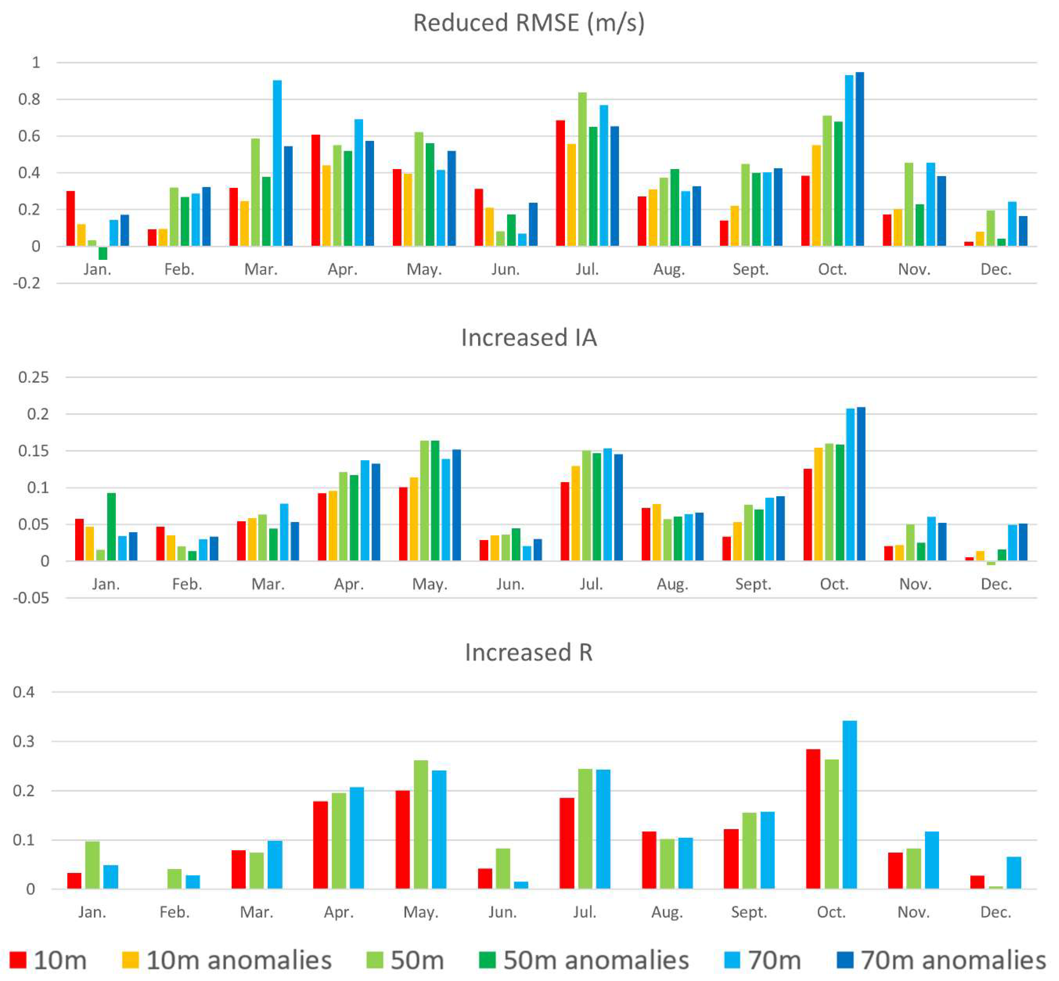
Compared with Test 1, we calculated the average reduced RMSE, increased IA and increased R of Test 2; the results of wind speed and wind speed anomalies are shown in Figure 10.
The RMSE results in Figure 10 show that March, April, May, July, and October reduced larger values of RMSE; and November, December, January, February, June reduced less RMSE. The results of IA and R are roughly the same as those of RMSE. Data assimilation can significantly improve the wind simulation results in March–May and July–October.
By comparing the results of wind speed and wind speed anomalies, we can find that the reduced RMSE values have gaps between the two results, especially in March, April, and July, when the reduced RMSE values of the anomalies results are smaller than the wind speed results. Moreover, Figure 9 shows that Test 2 has less mean speed bias than Test 1. This means that, in these months, some systematic bias was corrected by data assimilation.
From the Figure A1, Figure A2 and Figure A3 in Appendix B, we can find that during March–May and July–October, the main wind directions were south, southeast, and east, while the main wind directions during November–February were north, and the north wind during November–February had high speed and was very stable. Wind in the north direction may be caused by the winter monsoon. The winter monsoon is affected by large-scale circulation, and the effect of data assimilation may be limited.
From Figure 10, we can find that, in March–May and July–October, although the results in Test 1 differ greatly in different months, after data assimilation, the differences in Test 2 become smaller. Figure 10 shows that, compared with Test 1, Test 2 improved a lot in March, April, May, and October. Data assimilation can solve some of the bad cases of simulations in spring and autumn.
For the performance of data assimilation at different heights, we found that, compared with the lower level (10 m), most cases at the higher levels (50 and 70 m) have larger RMSE reductions and increments of IA and R. This result indicates that, through data assimilation, simulation results at higher levels improved more than those at lower levels. It can be seen from Figure 4 that the wind speed of 10 m is smaller than the wind speed of 50 and 70 m, so the error reduction is small. At the same time, the wind speed of 10 m is affected by the terrain, and the data assimilation has a greater effect on 50 and 70 m.
The incremental field can reflect the dynamic adjustments from data assimilation. To investigate the incremental field between Test 1 and Test 2, the MAD was calculated as follows:
where is the total grid number in domain 03; is the U or V wind speed of Test 2; and is the U or V wind speed of Test 1.
Figure 11 shows the vertical distribution of MAD between Test 1 and Test 2 in 00, 06, 12, and 18 UTC. We could find that, at each time, the MAD increased with the height and reached the maximum value at around 200–300 m height, and then decreased with height. The assimilation of satellite data has effects in the troposphere rather than just improving the near-surface layers. Moreover, the MAD of V component of wind speed is larger than U component, especially in 12 and 18 UTC. In our study case, the V component of wind speed is the direction of sea–land breeze, and it may be because that satellite data assimilation improved the temperature and pressure field and affected the simulation of sea–land breeze.
4. Discussion
In previous research, the simulation of wind speeds in coastal wind farm areas were mainly based on the direct simulation of WRF models with analysis data [27,35,36,37,38,39,40,41]. Since the parameters chosen for WRF can greatly affect the wind simulation, many studies have focused on the selection and improvement of the physical parameterization scheme of the WRF model [5,7,8]. However, another key factor affecting the model results is the initial field and real-time update of the model fields generated by the data assimilation system. Due to the uncertainty of wind speed changes near the surface, data assimilation has not been widely used in wind speed simulation. Our work used satellite data assimilation and improved the wind speed simulation results.
Wind resource assessment tasks require high quality of both wind speed distribution and time series of wind speed. Our results show that the Weibull distribution of Test 2 is closer to the observation than that of Test 1. Additionally, some statistical results were improved after data assimilation, indicating that the time series of wind speed can also be more accurate.
Application of data assimilation technology for wind speed simulation is a new trend in recent years. Our results show that data assimilation in different seasons has great differences in the improvement of wind simulation and the differences depend on the wind condition, and both systematic bias and random error can be corrected by satellite data assimilation.
5. Conclusions
In this paper, a one-year wind speed simulation was performed in the wind farm area of Yangjiang. Through the WRF-3DVar system, satellite data assimilation was applied to wind speed simulation in wind resource assessments. The errors and correlations between wind speed and wind speed anomalies in the two tests were compared through three indices—RMSE, IA, and R. Finally, we analyzed the differences of each index in different seasons. The main conclusions are as follows.
The Weibull distribution of Test 2 is closer to the observation than Test 1, and after applying data assimilation, the distribution of wind speed is more accurate.
According to the simulation results of the different seasons, it can be found that the wind simulation in the coastal areas of Guangdong has the best performance in summer and the worst performance in spring. This may be because the spring wind mainly comes from the ocean direction, and in winter and spring, there exist more systematic bias of the WRF model.
Compared to the conventional observations, the satellite data have greater geographic coverage, especially on the sea. The simulation results using satellite data assimilation can reduce the wind speed error and have better agreement with the observation data. Except for winter, the value of RMSE is greatly reduced in the other seasons. Comparing the wind speed and wind speed anomalies results, it can be seen that both the systematic bias and the random error were corrected. The IA and R between simulation results and observations are significantly improved in some months with very low correlations (April and May).
Because conventional observations are mainly distributed in inland synoptic observation stations, the performance of conventional data assimilation is less than the satellite data assimilation.
From the improvements of RMSE, IA, and R with data assimilation, it can be found that with the data assimilation, the performance of wind speed is improved in the spring and autumn, while the improvements are limited in winter. Data assimilation can significantly improve simulations during periods of poor simulation performance. From the wind distribution of the model result, we can find that the wind direction in winter was the same as the winter monsoon, and the systematic bias of the model was large during winter.
The wind speed improvements of data assimilation at the lower level (10 m) were less significant than that at the upper levels (50 and 70 m). This is because the wind near 10 m may be greatly affected by the terrain.
The current methods for wind resource assessment mainly use numerical models to simulate wind speed. Through this work, it can be found that data assimilation can be used to reduce simulation errors (both systematic bias and random errors) and to improve the correlation between simulation results and observations. Furthermore, the combined way of WRF-3Dvar can be applied in wind resource assessment for wind farm location selection and other applications.
Author Contributions
Conceptualization, Y.L.; methodology, W.X.; software, W.X.; validation, W.X.; formal analysis, W.X.; investigation, W.X.; resources, Y.L.; data curation, W.X.; writing—original draft preparation, W.X.; writing—review and editing, Y.L. and L.N.; visualization, W.X.; supervision, Y.L. and L.N.; project administration, Y.L.; funding acquisition, Y.L. All authors read and agreed to the published version of the manuscript.
Funding
This research was funded by the National Key Research and Development Program of China (2018YFB1502803) and the Scientific Research Program of Tsinghua University “Research on Wind Farm Weather Forecasting Technology for Power Grid”.
Acknowledgments
The wind observation data of the wind towers were provided by China Huaneng Group Co., Ltd. (CHNG), and the software of the tower data decoding was also provided by CHNG. The authors are very grateful for the observation data and its decoding software provided by CHNG. The FNL data were provided by CISL Research Data Archive (RDA) website (https://rda.ucar.edu/datasets/ds083.2/). The surface and upper-air observation data were also provided by CISL RDA (surface: https://rda.ucar.edu/datasets/ds461.0/ and upper air: https://rda.ucar.edu/datasets/ds351.0/). The authors are also grateful for the provider of these data.
Conflicts of Interest
The authors declare no conflicts of interest.
Appendix A

Table A1.
Statistical results of Test 1, Test 2, and Test 3, at 10 m height.
| Tower 1 | Tower 2 | Tower 3 | Tower 4 | Tower 5 | Tower 6 | Tower 7 | ||||||||||||||||
|---|---|---|---|---|---|---|---|---|---|---|---|---|---|---|---|---|---|---|---|---|---|---|
| Test 1 | Test 2 | Test 3 | Test 1 | Test 2 | Test 3 | Test 1 | Test 2 | Test 3 | Test 1 | Test 2 | Test 3 | Test 1 | Test 2 | Test 3 | Test 1 | Test 2 | Test 3 | Test 1 | Test 2 | Test 3 | ||
| Jan. | RMSE (m/s) | 2.80 | 2.33 | 2.47 | 3.23 | 2.90 | 3.10 | 3.22 | 2.98 | 3.08 | 3.38 | 3.22 | 3.28 | |||||||||
| IA | 0.65 | 0.77 | 0.73 | 0.55 | 0.59 | 0.57 | 0.66 | 0.70 | 0.68 | 0.60 | 0.64 | 0.63 | ||||||||||
| R | 0.64 * | 0.67 * | 0.66 * | 0.54 * | 0.50 * | 0.52 * | 0.54 * | 0.69 * | 0.62 * | 0.61 * | 0.60 * | 0.61 * | ||||||||||
| Feb. | RMSE (m/s) | 2.62 | 2.66 | 2.63 | 3.42 | 3.22 | 3.33 | 3.66 | 3.45 | 3.52 | 2.87 | 2.87 | 2.87 | |||||||||
| IA | 0.66 | 0.75 | 0.72 | 0.54 | 0.57 | 0.55 | 0.58 | 0.60 | 0.59 | 0.68 | 0.72 | 0.71 | ||||||||||
| R | 0.60 * | 0.57 * | 0.59 * | 0.41 * | 0.43 * | 0.42 * | 0.36 * | 0.44 * | 0.42 * | 0.68 * | 0.64 * | 0.66 * | ||||||||||
| Mar. | RMSE (m/s) | 3.64 | 2.96 | 3.24 | 4.13 | 3.51 | 3.70 | 2.63 | 2.87 | 2.72 | 2.73 | 2.72 | 2.72 | 4.21 | 3.70 | 3.95 | 3.84 | 3.19 | 3.40 | 2.71 | 2.74 | 2.71 |
| IA | 0.58 | 0.58 | 0.58 | 0.65 | 0.70 | 0.69 | 0.62 | 0.68 | 0.67 | 0.59 | 0.72 | 0.67 | 0.47 | 0.51 | 0.49 | 0.58 | 0.64 | 0.62 | 0.66 | 0.72 | 0.65 | |
| R | 0.36 * | 0.39 * | 0.38 * | 0.58 * | 0.72 * | 0.68 * | 0.41 * | 0.55 * | 0.50 * | 0.49 * | 0.54 * | 0.52 * | 0.24 * | 0.37 * | 0.30 * | 0.48 * | 0.55 * | 0.52 * | 0.59 * | 0.59 * | 0.59 * | |
| Apr. | RMSE (m/s) | 3.01 | 2.31 | 2.60 | 3.32 | 2.52 | 2.69 | 3.90 | 3.33 | 3.47 | 3.37 | 2.83 | 2.98 | 3.98 | 3.09 | 3.56 | 3.36 | 2.76 | 3.00 | 2.50 | 2.33 | 2.40 |
| IA | 0.46 | 0.62 | 0.56 | 0.46 | 0.63 | 0.59 | 0.57 | 0.63 | 0.62 | 0.59 | 0.62 | 0.61 | 0.44 | 0.57 | 0.50 | 0.51 | 0.63 | 0.58 | 0.58 | 0.58 | 0.58 | |
| R | 0.13 * | 0.40 * | 0.30 * | 0.15 * | 0.44 * | 0.37 * | 0.39 * | 0.54 * | 0.49 * | 0.37 * | 0.50 * | 0.46 * | 0.16 * | 0.48 * | 0.29 * | 0.24 * | 0.43 * | 0.35 * | 0.40 * | 0.33 * | 0.38 * | |
| May | RMSE (m/s) | 2.58 | 2.24 | 2.38 | 2.29 | 1.91 | 2.02 | 2.86 | 2.37 | 2.53 | 2.82 | 2.01 | 2.23 | 3.28 | 2.72 | 3.00 | 2.83 | 2.46 | 2.58 | 1.99 | 2.00 | 1.99 |
| IA | 0.56 | 0.64 | 0.61 | 0.49 | 0.65 | 0.60 | 0.51 | 0.63 | 0.60 | 0.48 | 0.69 | 0.63 | 0.47 | 0.58 | 0.52 | 0.48 | 0.59 | 0.54 | 0.64 | 0.58 | 0.65 | |
| R | 0.31 * | 0.48 * | 0.42 * | 0.17 * | 0.41 * | 0.35 * | 0.23 * | 0.44 * | 0.37 * | 0.13 * | 0.54 * | 0.44 * | 0.22 * | 0.50 * | 0.35 * | 0.17 * | 0.39 * | 0.33 * | 0.46 * | 0.33 * | 0.45 * | |
| Jun. | RMSE (m/s) | 2.29 | 2.06 | 2.15 | 2.31 | 2.02 | 2.09 | 2.84 | 2.56 | 2.64 | 2.53 | 2.04 | 2.20 | 3.39 | 2.87 | 3.16 | 3.34 | 3.17 | 3.23 | 2.32 | 2.12 | 2.18 |
| IA | 0.60 | 0.63 | 0.62 | 0.61 | 0.67 | 0.65 | 0.70 | 0.70 | 0.70 | 0.65 | 0.72 | 0.70 | 0.55 | 0.59 | 0.57 | 0.62 | 0.61 | 0.61 | 0.59 | 0.62 | 0.61 | |
| R | 0.36 * | 0.37 * | 0.37 * | 0.34 * | 0.45 * | 0.42 * | 0.58 * | 0.57 * | 0.58 * | 0.41 * | 0.56 * | 0.50 * | 0.36 * | 0.46 * | 0.41 * | 0.52 * | 0.49 * | 0.51 * | 0.48 * | 0.44 * | 0.47 * | |
| Jul. | RMSE(m/s) | 2.38 | 1.84 | 2.05 | 2.07 | 1.49 | 1.65 | 3.44 | 2.43 | 2.69 | 3.07 | 2.19 | 2.43 | 3.61 | 2.85 | 3.31 | 3.88 | 2.95 | 3.34 | 1.91 | 1.80 | 1.83 |
| IA | 0.65 | 0.77 | 0.72 | 0.59 | 0.76 | 0.71 | 0.58 | 0.76 | 0.70 | 0.47 | 0.57 | 0.53 | 0.47 | 0.60 | 0.53 | 0.38 | 0.47 | 0.44 | 0.69 | 0.67 | 0.68 | |
| R | 0.44 * | 0.66 * | 0.58 * | 0.32 * | 0.61 * | 0.54 * | 0.47 * | 0.74 * | 0.65 * | 0.26 * | 0.46 * | 0.40 * | 0.22 * | 0.48 * | 0.33 * | 0.03 | 0.24 * | 0.16 * | 0.63 * | 0.47 * | 0.64 * | |
| Aug. | RMSE (m/s) | 1.81 | 1.64 | 1.70 | 2.07 | 1.60 | 1.75 | 2.73 | 2.37 | 2.46 | 3.00 | 2.76 | 2.90 | 2.02 | 1.90 | 1.94 | ||||||
| IA | 0.82 | 0.86 | 0.85 | 0.73 | 0.86 | 0.82 | 0.65 | 0.75 | 0.71 | 0.64 | 0.71 | 0.67 | 0.61 | 0.63 | 0.62 | |||||||
| R | 0.70 * | 0.78 * | 0.75 * | 0.57 * | 0.77 * | 0.72 * | 0.51 * | 0.67 * | 0.63 * | 0.56 * | 0.69 * | 0.62 * | 0.44 * | 0.46 * | 0.45 * | |||||||
| Sept. | RMSE(m/s) | 2.39 | 2.16 | 2.25 | 2.59 | 2.40 | 2.44 | 2.90 | 2.84 | 2.85 | 2.89 | 2.58 | 2.75 | 2.24 | 2.32 | 2.26 | ||||||
| IA | 0.60 | 0.66 | 0.64 | 0.63 | 0.66 | 0.65 | 0.61 | 0.60 | 0.61 | 0.49 | 0.57 | 0.52 | 0.63 | 0.63 | 0.63 | |||||||
| R | 0.39 * | 0.60 * | 0.52 * | 0.51 * | 0.64 * | 0.60 * | 0.48 * | 0.58 * | 0.55 * | 0.20 * | 0.41 * | 0.30 * | 0.53 * | 0.47 * | 0.52 * | |||||||
| Oct. | RMSE (m/s) | 2.64 | 2.22 | 2.40 | 2.90 | 2.39 | 2.50 | 2.92 | 2.67 | 2.74 | 3.07 | 2.70 | 2.92 | 2.51 | 2.14 | 2.26 | ||||||
| IA | 0.62 | 0.75 | 0.70 | 0.55 | 0.71 | 0.68 | 0.60 | 0.69 | 0.67 | 0.50 | 0.64 | 0.55 | 0.56 | 0.68 | 0.63 | |||||||
| R | 0.41 * | 0.72 * | 0.60 * | 0.32 * | 0.64 * | 0.56 * | 0.43 * | 0.68 * | 0.62 * | 0.20 * | 0.54 * | 0.36 * | 0.31 * | 0.53 * | 0.46 * | |||||||
| Nov. | RMSE (m/s) | 3.04 | 2.81 | 2.89 | 3.21 | 2.91 | 3.00 | 4.09 | 3.92 | 3.96 | 3.76 | 3.43 | 3.59 | 2.92 | 3.08 | 2.97 | ||||||
| IA | 0.60 | 0.63 | 0.62 | 0.62 | 0.65 | 0.64 | 0.58 | 0.60 | 0.59 | 0.46 | 0.50 | 0.48 | 0.64 | 0.63 | 0.64 | |||||||
| R | 0.39 * | 0.51 * | 0.46 * | 0.54 * | 0.65 * | 0.62 * | 0.52 * | 0.63 * | 0.60 * | 0.24 * | 0.33 * | 0.29 * | 0.61 * | 0.56 * | 0.61 * | |||||||
| Dec. | RMSE (m/s) | 4.19 | 4.16 | 4.16 | 5.36 | 5.35 | 5.35 | 3.49 | 3.49 | 3.49 | 3.50 | 3.44 | 3.46 | |||||||||
| IA | 0.69 | 0.69 | 0.69 | 0.55 | 0.54 | 0.55 | 0.58 | 0.59 | 0.59 | 0.70 | 0.72 | 0.71 | ||||||||||
| R | 0.74 * | 0.77 * | 0.76 * | 0.56 * | 0.66 * | 0.62 * | 0.51 * | 0.50 * | 0.51 * | 0.69 * | 0.69 * | 0.69 * | ||||||||||
* The correlation coefficient has a confidence level of more than 99%.
Table A2.
Statistical results of Test 1, Test 2, and Test 3, at 50 m height.
| Tower 1 | Tower 2 | Tower 3 | Tower 4 | Tower 5 | Tower 6 | Tower 7 | |||||||||||||||||
|---|---|---|---|---|---|---|---|---|---|---|---|---|---|---|---|---|---|---|---|---|---|---|---|
| Test 1 | Test 2 | Test 3 | Test 1 | Test 2 | Test 3 | Test 1 | Test 2 | Test 3 | Test 1 | Test 2 | Test 3 | Test 1 | Test 2 | Test 3 | Test 1 | Test 2 | Test 3 | Test 1 | Test 2 | Test 3 | |||
| Jan. | RMSE (m/s) | 4.37 | 4.48 | 4.41 | 2.68 | 2.67 | 2.67 | 4.14 | 4.39 | 4.27 | 3.08 | 2.53 | 2.74 | 3.60 | 3.64 | 3.61 | |||||||
| IA | 0.72 | 0.72 | 0.72 | 0.78 | 0.73 | 0.76 | 0.33 | 0.40 | 0.35 | 0.69 | 0.77 | 0.75 | 0.69 | 0.67 | 0.68 | ||||||||
| R | 0.77 * | 0.81 * | 0.80 * | 0.68 * | 0.61 * | 0.66 * | 0.15 | 0.50 * | 0.09 | 0.47 * | 0.60 * | 0.55 * | 0.63 * | 0.67 * | 0.67 * | ||||||||
| Feb. | RMSE (m/s) | 3.98 | 3.60 | 3.70 | 3.13 | 2.83 | 2.91 | 3.74 | 3.18 | 3.38 | 3.41 | 3.38 | 3.39 | ||||||||||
| IA | 0.69 | 0.76 | 0.74 | 0.74 | 0.72 | 0.73 | 0.56 | 0.63 | 0.61 | 0.73 | 0.70 | 0.72 | |||||||||||
| R | 0.66 * | 0.69 * | 0.68 * | 0.60 * | 0.60 * | 0.60 * | 0.26 * | 0.35 * | 0.32 * | 0.61 * | 0.63 * | 0.63 * | |||||||||||
| Mar. | RMSE (m/s) | 3.97 | 2.73 | 3.20 | 4.18 | 3.09 | 3.32 | 3.81 | 4.05 | 3.88 | 2.86 | 2.75 | 2.78 | 3.51 | 2.58 | 2.93 | 3.66 | 3.26 | 3.39 | ||||
| IA | 0.60 | 0.66 | 0.63 | 0.65 | 0.76 | 0.73 | 0.68 | 0.70 | 0.69 | 0.67 | 0.77 | 0.73 | 0.62 | 0.73 | 0.70 | 0.70 | 0.68 | 0.69 | |||||
| R | 0.38 * | 0.37 * | 0.37 * | 0.45 * | 0.66 * | 0.60 * | 0.59 * | 0.60 * | 0.60 * | 0.50 * | 0.59 * | 0.56 * | 0.42 * | 0.53 * | 0.49 * | 0.57 * | 0.60 * | 0.60 * | |||||
| Apr. | RMSE (m/s) | 3.50 | 2.52 | 2.84 | 3.38 | 2.60 | 2.77 | 4.37 | 4.54 | 4.42 | 3.52 | 3.00 | 3.16 | 3.12 | 2.64 | 2.79 | 3.65 | 2.94 | 3.23 | ||||
| IA | 0.50 | 0.71 | 0.63 | 0.51 | 0.70 | 0.64 | 0.61 | 0.64 | 0.63 | 0.62 | 0.68 | 0.66 | 0.59 | 0.71 | 0.67 | 0.60 | 0.72 | 0.68 | |||||
| R | 0.20 * | 0.51 * | 0.40 * | 0.20 * | 0.51 * | 0.42 * | 0.39 * | 0.52 * | 0.48 * | 0.40 * | 0.48 * | 0.46 * | 0.33 * | 0.50 * | 0.44 * | 0.40 * | 0.58 * | 0.51 * | |||||
| May | RMSE (m/s) | 2.58 | 1.96 | 2.23 | 2.89 | 2.45 | 2.55 | 3.25 | 2.26 | 2.52 | 3.01 | 2.37 | 2.59 | 2.93 | 2.48 | 2.61 | 2.72 | 2.14 | 2.31 | ||||
| IA | 0.59 | 0.77 | 0.71 | 0.52 | 0.67 | 0.63 | 0.44 | 0.59 | 0.53 | 0.52 | 0.72 | 0.65 | 0.51 | 0.64 | 0.59 | 0.56 | 0.74 | 0.68 | |||||
| R | 0.34 * | 0.61 * | 0.52 * | 0.24 * | 0.49 * | 0.43 * | 0.13 * | 0.31 * | 0.27 * | 0.21 * | 0.57 * | 0.47 * | 0.21 * | 0.42 * | 0.35 * | 0.28 * | 0.58 * | 0.47 * | |||||
| Jun. | RMSE (m/s) | 2.54 | 2.53 | 2.54 | 2.79 | 2.68 | 2.71 | 2.72 | 2.97 | 2.77 | 2.84 | 2.55 | 2.66 | 3.12 | 2.88 | 2.97 | 2.87 | 2.77 | 2.80 | ||||
| IA | 0.66 | 0.67 | 0.67 | 0.60 | 0.63 | 0.62 | 0.49 | 0.61 | 0.57 | 0.69 | 0.74 | 0.73 | 0.71 | 0.72 | 0.72 | 0.68 | 0.69 | 0.69 | |||||
| R | 0.49 * | 0.48 * | 0.49 * | 0.35 * | 0.43 * | 0.41 * | 0.13 * | 0.37 * | 0.29 * | 0.47 * | 0.57 * | 0.54 * | 0.58 * | 0.57 * | 0.57 * | 0.45 * | 0.52 * | 0.49 * | |||||
| Jul. | RMSE (m/s) | 2.65 | 1.93 | 2.21 | 2.38 | 1.89 | 2.03 | 3.35 | 2.56 | 3.01 | 3.03 | 1.78 | 2.27 | 4.00 | 2.79 | 3.31 | 2.80 | 2.24 | 2.42 | ||||
| IA | 0.69 | 0.83 | 0.78 | 0.59 | 0.73 | 0.69 | 0.62 | 0.87 | 0.79 | 0.50 | 0.68 | 0.62 | 0.40 | 0.49 | 0.45 | 0.70 | 0.80 | 0.77 | |||||
| R | 0.48 * | 0.71 * | 0.63 * | 0.31 * | 0.59 * | 0.52 * | 0.51 * | 0.79 * | 0.72 * | 0.28 * | 0.50 * | 0.44 * | 0.02 | 0.28 * | 0.18 * | 0.52 * | 0.71 * | 0.66 * | |||||
| Aug. | RMSE(m/s) | 2.01 | 1.86 | 1.92 | 2.34 | 1.91 | 2.03 | 3.58 | 2.43 | 2.80 | 2.47 | 2.71 | 2.56 | ||||||||||
| IA | 0.86 | 0.89 | 0.88 | 0.78 | 0.88 | 0.86 | 0.82 | 0.94 | 0.91 | 0.65 | 0.63 | 0.64 | |||||||||||
| R | 0.74 * | 0.80 * | 0.77 * | 0.62 * | 0.79 * | 0.74 * | 0.70 * | 0.89 * | 0.83 * | 0.44 * | 0.44 * | 0.44 * | |||||||||||
| Sept. | RMSE (m/s) | 2.42 | 1.90 | 2.10 | 2.77 | 2.42 | 2.51 | 3.33 | 2.59 | 2.85 | 2.58 | 2.41 | 2.46 | ||||||||||
| IA | 0.65 | 0.77 | 0.73 | 0.65 | 0.72 | 0.70 | 0.59 | 0.69 | 0.66 | 0.71 | 0.73 | 0.73 | |||||||||||
| R | 0.43 * | 0.62 * | 0.54 * | 0.42 * | 0.57 * | 0.53 * | 0.45 * | 0.66 * | 0.60 * | 0.56 * | 0.64 * | 0.61 * | |||||||||||
| Oct. | RMSE (m/s) | 2.74 | 1.77 | 2.14 | 3.28 | 2.35 | 2.60 | 2.74 | 2.40 | 2.52 | 3.23 | 2.63 | 2.82 | ||||||||||
| IA | 0.66 | 0.87 | 0.79 | 0.54 | 0.78 | 0.73 | 0.65 | 0.67 | 0.66 | 0.57 | 0.74 | 0.68 | |||||||||||
| R | 0.44 * | 0.78 * | 0.65 * | 0.24 * | 0.65 * | 0.53 * | 0.48 * | 0.51 * | 0.50 * | 0.32 * | 0.60 * | 0.49 * | |||||||||||
| Nov. | RMSE (m/s) | 3.09 | 2.62 | 2.81 | 2.97 | 2.65 | 2.74 | 3.67 | 3.03 | 3.20 | 3.50 | 3.10 | 3.26 | ||||||||||
| IA | 0.63 | 0.70 | 0.67 | 0.67 | 0.70 | 0.69 | 0.47 | 0.53 | 0.52 | 0.65 | 0.69 | 0.68 | |||||||||||
| R | 0.38 * | 0.50 * | 0.46 * | 0.47 * | 0.56 * | 0.54 * | 0.22 * | 0.26 * | 0.25 * | 0.55 * | 0.63 * | 0.60 * | |||||||||||
| Dec. | RMSE (m/s) | 3.16 | 3.07 | 3.10 | 4.31 | 3.85 | 4.02 | 3.91 | 3.88 | 3.89 | |||||||||||||
| IA | 0.81 | 0.81 | 0.81 | 0.62 | 0.62 | 0.62 | 0.76 | 0.74 | 0.75 | ||||||||||||||
| R | 0.72 * | 0.74 * | 0.73 * | 0.71 * | 0.71 * | 0.71 * | 0.72 * | 0.73 * | 0.73 * | ||||||||||||||
* The correlation coefficient has a confidence level of more than 99%.
Table A3.
Statistical results of Test 1, Test 2, and Test 3, at 70 m height.
| Tower 1 | Tower 2 | Tower 3 | Tower 4 | Tower 5 | Tower 6 | Tower 7 | |||||||||||||||||
|---|---|---|---|---|---|---|---|---|---|---|---|---|---|---|---|---|---|---|---|---|---|---|---|
| Test 1 | Test 2 | Test 3 | Test 1 | Test 2 | Test 3 | Test 1 | Test 2 | Test 3 | Test 1 | Test 2 | Test 3 | Test 1 | Test 2 | Test 3 | Test 1 | Test 2 | Test 3 | Test 1 | Test 2 | Test 3 | |||
| Jan. | RMSE (m/s) | 2.55 | 2.58 | 2.56 | 3.52 | 3.04 | 3.22 | 3.54 | 3.56 | 3.55 | |||||||||||||
| IA | 0.73 | 0.76 | 0.75 | 0.66 | 0.72 | 0.69 | 0.69 | 0.70 | 0.69 | ||||||||||||||
| R | 0.56 * | 0.62 * | 0.60 * | 0.42 * | 0.54 * | 0.49 * | 0.66 * | 0.62 * | 0.66 * | ||||||||||||||
| Feb. | RMSE (m/s) | 3.09 | 2.69 | 2.83 | 4.19 | 3.63 | 3.81 | 3.36 | 3.45 | 3.39 | |||||||||||||
| IA | 0.72 | 0.73 | 0.73 | 0.52 | 0.58 | 0.56 | 0.71 | 0.74 | 0.73 | ||||||||||||||
| R | 0.54 * | 0.56 * | 0.56 * | 0.19 * | 0.28 * | 0.25 * | 0.61 * | 0.59 * | 0.61 * | ||||||||||||||
| Mar. | RMSE (m/s) | 4.09 | 2.82 | 3.33 | 4.78 | 3.35 | 3.77 | 4.07 | 2.80 | 3.21 | 2.88 | 2.88 | 2.88 | 3.64 | 2.77 | 3.08 | 3.86 | 3.27 | 3.47 | ||||
| IA | 0.62 | 0.68 | 0.66 | 0.59 | 0.73 | 0.69 | 0.58 | 0.66 | 0.64 | 0.63 | 0.72 | 0.69 | 0.64 | 0.73 | 0.69 | 0.69 | 0.70 | 0.69 | |||||
| R | 0.42 * | 0.40 * | 0.41 * | 0.35 * | 0.60 * | 0.53 * | 0.37 * | 0.43 * | 0.41 * | 0.39 * | 0.52 * | 0.48 * | 0.41 * | 0.53 * | 0.49 * | 0.55 * | 0.60 * | 0.58 * | |||||
| Apr. | RMSE (m/s) | 4.08 | 2.61 | 3.16 | 3.72 | 2.89 | 3.09 | 3.82 | 2.98 | 3.28 | 3.18 | 3.01 | 3.05 | 2.99 | 2.64 | 2.74 | 3.56 | 3.10 | 3.25 | ||||
| IA | 0.48 | 0.75 | 0.65 | 0.48 | 0.67 | 0.63 | 0.60 | 0.73 | 0.69 | 0.63 | 0.67 | 0.65 | 0.50 | 0.62 | 0.57 | 0.62 | 0.70 | 0.66 | |||||
| R | 0.16 * | 0.57 * | 0.39 * | 0.15 * | 0.46 * | 0.38 * | 0.38 * | 0.55 * | 0.49 * | 0.38 * | 0.46 * | 0.43 * | 0.18 * | 0.35 * | 0.28 * | 0.42 * | 0.52 * | 0.48 * | |||||
| May | RMSE (m/s) | 2.58 | 2.01 | 2.23 | 3.12 | 2.64 | 2.76 | 2.78 | 2.23 | 2.41 | 2.92 | 2.49 | 2.64 | 2.63 | 2.58 | 2.60 | |||||||
| IA | 0.61 | 0.78 | 0.71 | 0.50 | 0.66 | 0.61 | 0.60 | 0.74 | 0.70 | 0.53 | 0.71 | 0.65 | 0.54 | 0.58 | 0.57 | ||||||||
| R | 0.35 * | 0.62 * | 0.53 * | 0.19 * | 0.45 * | 0.37 * | 0.34 * | 0.56 * | 0.48 * | 0.21 * | 0.58 * | 0.48 * | 0.22 * | 0.32 * | 0.29 * | ||||||||
| Jun. | RMSE (m/s) | 2.71 | 2.62 | 2.66 | 3.13 | 3.01 | 3.05 | 2.71 | 2.70 | 2.70 | 2.67 | 2.61 | 2.63 | ||||||||||
| IA | 0.67 | 0.69 | 0.68 | 0.56 | 0.59 | 0.58 | 0.75 | 0.77 | 0.76 | 0.72 | 0.73 | 0.73 | |||||||||||
| R | 0.52 * | 0.51 * | 0.52 * | 0.28 * | 0.37 * | 0.35 * | 0.58 * | 0.61 * | 0.60 * | 0.59 * | 0.54 * | 0.57 * | |||||||||||
| Jul. | RMSE (m/s) | 2.65 | 1.94 | 2.22 | 2.70 | 2.14 | 2.30 | 3.18 | 2.21 | 2.53 | 2.65 | 1.82 | 2.07 | ||||||||||
| IA | 0.71 | 0.84 | 0.79 | 0.55 | 0.71 | 0.67 | 0.68 | 0.84 | 0.79 | 0.54 | 0.69 | 0.64 | |||||||||||
| R | 0.50 * | 0.73 * | 0.65 * | 0.25 * | 0.57 * | 0.49 * | 0.50 * | 0.75 * | 0.67 * | 0.33 * | 0.50 * | 0.44 * | |||||||||||
| Aug. | RMSE (m/s) | 2.09 | 1.93 | 1.99 | 2.51 | 2.15 | 2.23 | 2.56 | 2.18 | 2.28 | |||||||||||||
| IA | 0.85 | 0.89 | 0.88 | 0.79 | 0.87 | 0.84 | 0.79 | 0.86 | 0.84 | ||||||||||||||
| R | 0.73 * | 0.80 * | 0.77 * | 0.63 * | 0.78 * | 0.73 * | 0.65 * | 0.74 * | 0.71 * | ||||||||||||||
| Sept. | RMSE (m/s) | 2.46 | 1.98 | 2.15 | 3.06 | 2.69 | 2.79 | 2.71 | 2.34 | 2.44 | |||||||||||||
| IA | 0.66 | 0.78 | 0.73 | 0.62 | 0.70 | 0.68 | 0.73 | 0.80 | 0.77 | ||||||||||||||
| R | 0.44 * | 0.62 * | 0.55 * | 0.37 * | 0.53 * | 0.49 * | 0.58 * | 0.71 * | 0.67 * | ||||||||||||||
| Oct. | RMSE (m/s) | 2.84 | 1.85 | 2.24 | 3.67 | 2.67 | 2.96 | 3.16 | 2.35 | 2.62 | |||||||||||||
| IA | 0.67 | 0.88 | 0.79 | 0.51 | 0.77 | 0.71 | 0.68 | 0.84 | 0.78 | ||||||||||||||
| R | 0.45 * | 0.79 * | 0.65 * | 0.19 * | 0.62 * | 0.51 * | 0.50 * | 0.75 * | 0.67 * | ||||||||||||||
| Nov. | RMSE (m/s) | 3.18 | 2.72 | 2.90 | 3.30 | 2.98 | 3.05 | 3.56 | 2.97 | 3.14 | |||||||||||||
| IA | 0.63 | 0.70 | 0.67 | 0.63 | 0.66 | 0.65 | 0.67 | 0.75 | 0.73 | ||||||||||||||
| R | 0.37 * | 0.49 * | 0.44 * | 0.39 * | 0.48 * | 0.46 * | 0.50 * | 0.65 * | 0.61 * | ||||||||||||||
| Dec. | RMSE (m/s) | 3.35 | 3.23 | 3.26 | 3.70 | 3.34 | 3.42 | ||||||||||||||||
| IA | 0.79 | 0.79 | 0.79 | 0.59 | 0.69 | 0.66 | |||||||||||||||||
| R | 0.67 * | 0.68 * | 0.68 * | 0.41 * | 0.53 * | 0.48 * | |||||||||||||||||
* The correlation coefficient has a confidence level of more than 99%.
Appendix B
Figure A1.
Wind rose of the Test 2 results in the seven tower positions in spring (Mar., Apr., and May).
Figure A1.
Wind rose of the Test 2 results in the seven tower positions in spring (Mar., Apr., and May).

Figure A2.
Wind rose of Test 2 results in the seven tower positions in summer (Jun., Jul., and Aug.).
Figure A2.
Wind rose of Test 2 results in the seven tower positions in summer (Jun., Jul., and Aug.).

Figure A3.
Wind rose of Test 2 results in the seven tower positions in autumn (Sept., Oct., and Nov.).
Figure A3.
Wind rose of Test 2 results in the seven tower positions in autumn (Sept., Oct., and Nov.).

Figure A4.
Wind rose of Test 2 results in the seven tower positions in winter (Dec., Jan., and Feb.)
Figure A4.
Wind rose of Test 2 results in the seven tower positions in winter (Dec., Jan., and Feb.)

References
- WWEA. Wind Power Capacity Worldwide Reaches 597 GW, 50,1 GW added in 2018. Available online: https://wwindea.org/blog/2019/02/25/wind-power-capacity-worldwide-reaches-600-gw-539-gw-added-in-2018/ (accessed on 27 December 2019).
- Costa, A.; Crespo, A.; Navarro, J.; Lizcano, G.; Madsen, H.; Feitosa, E. A review on the young history of the wind power short-term prediction. Renew. Sustain. Energy Rev. 2008, 12, 1725–1744. [Google Scholar] [CrossRef] [Green Version]
- Storm, B.; Dudhia, J.; Basu, S.; Swift, A.; Giammanco, I. Evaluation of the weather research and forecasting model on forecasting low-level jets: Implications for wind energy. Wind Energy Int. J. Prog. Appl. Wind Power Convers. Technol. 2009, 12, 81–90. [Google Scholar] [CrossRef]
- Skamarock, W.C.; Klemp, J.B.; Dudhia, J.; Gill, D.O.; Barker, D.M.; Wang, W.; Powers, J.G. A Description of the Advanced Research WRF Version 3. NCAR Technical Note-475+ STR. 2008. Available online: http://citeseerx.ist.psu.edu/viewdoc/summary?doi=10.1.1.484.3656 (accessed on 11 December 2018).
- Hu, X.; Nielsen-Gammon, J.W.; Zhang, F. Evaluation of Three Planetary Boundary Layer Schemes in the WRF Model. J. Appl. Meteorol. Clim. 2010, 49, 1831–1844. [Google Scholar] [CrossRef] [Green Version]
- Sušelj, K.; Sood, A. Improving the Mellor-Yamada-Janjić parameterization for wind conditions in the marine planetary boundary layer. Bound. Layer Meteorol. 2010, 136, 301–324. [Google Scholar] [CrossRef]
- Deppe, A.J.; Gallus, W.A., Jr.; Takle, E.S. A WRF ensemble for improved wind speed forecasts at turbine height. Weather Forecast. 2013, 28, 212–228. [Google Scholar] [CrossRef]
- Hu, X.M.; Klein, P.M.; Xue, M. Evaluation of the updated YSU planetary boundary layer scheme within WRF for wind resource and air quality assessments. J. Geophys. Res. Atmos. 2013, 118, 10–490. [Google Scholar] [CrossRef]
- Liu, Y.; Warner, T.; Liu, Y.; Vincent, C.; Wu, W.; Mahoney, B.; Swerdlin, S.; Parks, K.; Boehnert, J. Simultaneous nested modeling from the synoptic scale to the LES scale for wind energy applications. J. Wind Eng. Ind. Aerodyn. 2011, 99, 308–319. [Google Scholar] [CrossRef] [Green Version]
- Zhang, F.; Yang, Y.; Wang, C. The Effects of Assimilating Conventional and ATOVS Data on Forecasted Near-Surface Wind with WRF-3DVAR. Mon. Weather Rev. 2015, 143, 153–164. [Google Scholar] [CrossRef]
- Ancell, B.C.; Kashawlic, E.; Schroeder, J.L. Evaluation of wind forecasts and observation impacts from variational and ensemble data assimilation for wind energy applications. Mon. Weather Rev. 2015, 143, 3230–3245. [Google Scholar] [CrossRef]
- Ulazia, A.; Saenz, J.; Ibarra-Berastegui, G. Sensitivity to the use of 3DVAR data assimilation in a mesoscale model for estimating offshore wind energy potential. A case study of the Iberian northern coastline. Appl. Energy 2016, 180, 617–627. [Google Scholar] [CrossRef]
- Che, Y.; Xiao, F. An integrated wind-forecast system based on the weather research and forecasting model, Kalman filter, and data assimilation with nacelle-wind observation. J. Renew. Sustain. Energy 2016, 8, 53308. [Google Scholar] [CrossRef]
- Ulazia, A.; Sáenz, J.; Ibarra-Berastegui, G.; González-Rojí, S.J.; Carreno-Madinabeitia, S. Using 3DVAR data assimilation to measure offshore wind energy potential at different turbine heights in the West Mediterranean. Appl. Energy 2017, 208, 1232–1245. [Google Scholar] [CrossRef] [Green Version]
- Cheng, W.Y.; Liu, Y.; Bourgeois, A.J.; Wu, Y.; Haupt, S.E. Short-term wind forecast of a data assimilation/weather forecasting system with wind turbine anemometer measurement assimilation. Renew. Energy 2017, 107, 340–351. [Google Scholar] [CrossRef]
- China Meteorological Administration Wind Energy Solar Energy Resource Center. Detailed investigation and assessment of wind energy resources in China. Wind Energy 2011, 8, 26–30. (In Chinese) [Google Scholar]
- Morrison, H.; Thompson, G.; Tatarskii, V. Impact of cloud microphysics on the development of trailing stratiform precipitation in a simulated squall line: Comparison of one-and two-moment schemes. Mon. Weather Rev. 2009, 137, 991–1007. [Google Scholar] [CrossRef] [Green Version]
- Iacono, M.J.; Delamere, J.S.; Mlawer, E.J.; Shephard, M.W.; Clough, S.A.; Collins, W.D. Radiative forcing by long-lived greenhouse gases: Calculations with the AER radiative transfer models. J. Geophys. Res. Atmos. 2008, 113. [Google Scholar] [CrossRef]
- Ek, M.B.; Mitchell, K.E.; Lin, Y.; Rogers, E.; Grunmann, P.; Koren, V.; Gayno, G.; Tarpley, J.D. Implementation of Noah land surface model advances in the National Centers for Environmental Prediction operational mesoscale Eta model. J. Geophys. Res. Atmos. 2003, 108, GCP12-1. [Google Scholar] [CrossRef]
- Kain, J.S. The Kain—Fritsch convective parameterization: An update. J. Appl. Meteorol. 2004, 43, 170–181. [Google Scholar] [CrossRef] [Green Version]
- Hong, S.; Noh, Y.; Dudhia, J. A new vertical diffusion package with an explicit treatment of entrainment processes. Mon. Weather Rev. 2006, 134, 2318–2341. [Google Scholar] [CrossRef] [Green Version]
- National Centers for Environmental Prediction; National Weather Service; NOAA; U.S Department of Commerce. NCEP FNL Operational Model Global Tropospheric Analyses, Continuing from July 1999. Research Data Archive at the National Center for Atmospheric Research, Computational and Information Systems Laboratory. 2000. Available online: https://rda.ucar.edu/datasets/ds083.2/ (accessed on 11 December 2018).
- Parrish, D.F.; Derber, J.C. The National Meteorological Center’s spectral statistical-interpolation analysis system. Mon. Weather Rev. 1992, 120, 1747–1763. [Google Scholar] [CrossRef]
- National Centers for Environmental Prediction; National Weather Service; NOAA; U.S Department of Commerce. NCEP GDAS Satellite Data 2004-Continuing. Research Data Archive at the National Center for Atmospheric Research, Computational and Information Systems Laboratory, Boulder, Colo. (Updated daily). 2009. Available online: https://rda.ucar.edu/datasets/ds735.0/ (accessed on 11 December 2018).
- National Centers for Environmental Prediction; National Weather Service; NOAA; U.S Department of Commerce. Updated Daily. NCEP ADP Global Surface Observational Weather Data, October 1999-continuing. Research Data Archive at the National Center for Atmospheric Research, Computational and Information Systems Laboratory. 2004. Available online: https://data.ucar.edu/dataset/ncep-adp-global-surface-observational-weather-data-october-1999-continuing (accessed on 2 March 2020).
- National Centers for Environmental Prediction; National Weather Service; NOAA; U.S Department of Commerce. Updated Daily. NCEP ADP Global Upper Air Observational Weather Data, October 1999-Continuing. Research Data Archive at the National Center for Atmospheric Research, Computational and Information Systems Laboratory. 2004. Available online: https://data.ucar.edu/dataset/ncep-adp-global-upper-air-observational-weather-data-october-1999-continuing (accessed on 2 March 2020).
- Carvalho, D.; Rocha, A.; Gómez-Gesteira, M.; Santos, C. A sensitivity study of the WRF model in wind simulation for an area of high wind energy. Environ. Model. Softw. 2012, 33, 23–34. [Google Scholar] [CrossRef] [Green Version]
- Willmott, C.J. On the validation of models. Phys. Geogr. 1981, 2, 184–194. [Google Scholar] [CrossRef]
- Willmott, C.J. On the evaluation of model performance in physical geography. In Spatial Statistics and Models; Gaile, G.L., Willmott, C.J., Eds.; Springer: Dordrecht, The Netherlands, 1984; pp. 443–460. [Google Scholar]
- Willmott, C.J.; Ackleson, S.G.; Davis, R.E.; Feddema, J.J.; Klink, K.M.; Legates, D.R.; O’Donnell, J.; Rowe, C.M. Statistics for the evaluation and comparison of models. J. Geophys. Res. Ocean. 1985, 90, 8995–9005. [Google Scholar] [CrossRef] [Green Version]
- Legates, D.R.; McCabe, G.J., Jr. Evaluating the use of “goodness-of-fit” measures in hydrologic and hydroclimatic model validation. Water Resour. Res. 1999, 35, 233–241. [Google Scholar] [CrossRef]
- Lun, I.Y.F.; Lam, J.C. A study of Weibull parameters using long-term wind observations. Renew. Energy 2000, 20, 145–153. [Google Scholar] [CrossRef]
- Stensrud, D.J.; Skindlov, J.A. Gridpoint predictions of high temperature from a mesoscale model. Weather Forecast. 1996, 11, 103–110. [Google Scholar] [CrossRef] [Green Version]
- Anthes, R.A.; Warner, T.T. Development of hydrodynamic models suitable for air pollution and other mesometerological studies. Mon. Weather Rev. 1978, 106, 1045–1078. [Google Scholar] [CrossRef] [Green Version]
- Carvalho, D.; Rocha, A.; Gómez-Gesteira, M. Ocean surface wind simulation forced by different reanalyses: Comparison with observed data along the Iberian Peninsula coast. Ocean Model. 2012, 56, 31–42. [Google Scholar] [CrossRef]
- Carvalho, D.; Rocha, A.; Santos, C.S.; Pereira, R. Wind resource modelling in complex terrain using different mesoscale–microscale coupling techniques. Appl. Energy 2013, 108, 493–504. [Google Scholar] [CrossRef] [Green Version]
- Carvalho, D.; Rocha, A.; Gómez-Gesteira, M.; Silva Santos, C. WRF wind simulation and wind energy production estimates forced by different reanalyses: Comparison with observed data for Portugal. Appl. Energy 2014, 117, 116–126. [Google Scholar] [CrossRef]
- Carvalho, D.; Rocha, A.; Gómez-Gesteira, M.; Silva Santos, C. Offshore wind energy resource simulation forced by different reanalyses: Comparison with observed data in the Iberian Peninsula. Appl. Energy 2014, 134, 57–64. [Google Scholar] [CrossRef]
- Mattar, C.; Borvar, D. Offshore wind power simulation by using WRF in the central coast of Chile. Renew. Energy 2016, 94, 22–31. [Google Scholar] [CrossRef]
- Giannaros, T.M.; Melas, D.; Ziomas, I. Performance evaluation of the Weather Research and Forecasting (WRF) model for assessing wind resource in Greece. Renew. Energy 2017, 102, 190–198. [Google Scholar] [CrossRef]
- Salvação, N.; Soares, C.G. Wind resource assessment offshore the Atlantic Iberian coast with the WRF model. Energy 2018, 145, 276–287. [Google Scholar] [CrossRef]
Figure 1.
Terrain height of inner domain and the distribution of the seven wind observation towers (red dots). “T1” represents Tower 1, “T2” represents Tower 2, and so forth.
Figure 1.
Terrain height of inner domain and the distribution of the seven wind observation towers (red dots). “T1” represents Tower 1, “T2” represents Tower 2, and so forth.

Figure 2.
Terrain height of the model’s simulation domains. There are three nested domains: domain 01 (d01), domain 02 (d02), and domain 03 (d03).
Figure 2.
Terrain height of the model’s simulation domains. There are three nested domains: domain 01 (d01), domain 02 (d02), and domain 03 (d03).

Figure 3.
Locations of synoptic observation stations (red dots).

Figure 4.
Model running process for Tests 1, 2, and 3. Test 1 (left) started the model at 18:00 UTC every day, with 6 h spin up and 24 h model run. Tests 2 and 3 (right) started the model at 18:00 UTC every day and assimilated satellite/conventional data at 18:00 UTC, 00:00 UTC (+1day), 06:00 UTC (+1day), 12:00 UTC (+1day), and 18:00 UTC (+1day).

Figure 5.
Mean absolute difference (MAD) of U (m/s) and V (m/s) at different heights (10, 50, and 70 m) in Test 2.
Figure 5.
Mean absolute difference (MAD) of U (m/s) and V (m/s) at different heights (10, 50, and 70 m) in Test 2.

Figure 6.
The Weibull distribution of seven towers at different heights. The blue lines are the observed wind speeds, the green lines are the results of Test 1 (no data assimilation), and the red lines are the results of Test 2 (data assimilation).
Figure 6.
The Weibull distribution of seven towers at different heights. The blue lines are the observed wind speeds, the green lines are the results of Test 1 (no data assimilation), and the red lines are the results of Test 2 (data assimilation).

Figure 7.
Average of the results of root-mean-square error (RMSE), index of agreement (IA), and Correlation Coefficient (R) from the seven towers.
Figure 7.
Average of the results of root-mean-square error (RMSE), index of agreement (IA), and Correlation Coefficient (R) from the seven towers.

Figure 8.
Average results of root-mean-square error (RMSE), index of agreement (IA), and correlation coefficient (R) in Test 1; “10 m”, “50 m”, “70 m” are the RMSE, IA, and R results of wind speed at 10, 50, and 70 m, and the “anomalies” histograms are the results of RMSE, IA, and R, calculated using wind speed anomalies.

Figure 9.
Average of the results of the mean speed bias from the seven towers.

Figure 10.
Difference between Test 2 and Test 1 results; “10 m”, “50 m”, and “70 m” are the reduced root-mean-square error (RMSE), increased index of agreement (IA), and increased correlation coefficient (R) results of wind speed at 10, 50, and 70 m. The “anomalies” histograms are the results of the reduced RMSE, increased IA, and increased R calculated using wind speed anomalies in Test 1 and Test 2.

Figure 11.
Vertical distribution of mean absolute difference (MAD) of U (m/s) and V (m/s) between Test 1 and Test 2 in 00 UTC (a) 06 UTC (b) 12 UTC (c), and 18 UTC (d).
Figure 11.
Vertical distribution of mean absolute difference (MAD) of U (m/s) and V (m/s) between Test 1 and Test 2 in 00 UTC (a) 06 UTC (b) 12 UTC (c), and 18 UTC (d).

Table 1.
Latitude, longitude, and terrain height of wind observation towers.
| Tower | Longitude (E) | Latitude (N) | Terrain Height (m) |
|---|---|---|---|
| Tower1 | 112.304 | 21.768 | 380 |
| Tower2 | 112.309 | 21.827 | 285 |
| Tower3 | 112.208 | 21.783 | 320 |
| Tower4 | 111.985 | 22.144 | 540 |
| Tower5 | 112.269 | 21.796 | 473 |
| Tower6 | 112.076 | 22.110 | 758 |
| Tower7 | 112.334 | 21.844 | 322 |
Table 2.
Wind towers’ sensor type, model number, hardware version, and software version.
| Tower | Wind Sensor | Model | Hardware version | Software Version | Sampling Frequency | Sensor Bias |
|---|---|---|---|---|---|---|
| Tower 1 | NRG | 4280 | 023-022-053 | SDR 6.0.26 | 1 s | |
| Tower 2 | NRG | 4280 | 023-022-053 | SDR 6.0.26 | 1 s | |
| Tower 3 | NRG | 4280 | 023-022-036 | SDR 6.0.26 | 1 s | |
| Tower 4 | NRG | 4280 | 023-022-036 | SDR 6.0.26 | 1 s | |
| Tower 5 | NRG | 4280 | 023-022-039 | SDR 6.0.26 | 1 s | |
| Tower 6 | NRG | 4280 | 023-022-039 | SDR 6.0.26 | 1 s | |
| Tower 7 | NRG | 4280 | 023-022-039 | SDR 6.0.26 | 1 s |
Table 3.
The number of wind speed observations’ original data in different months of the year 2012. Each tower has height levels of 10, 50, and 70 m.
Table 3.
The number of wind speed observations’ original data in different months of the year 2012. Each tower has height levels of 10, 50, and 70 m.
| Station 1 | Station 2 | Station 3 | Station 4 | Station 5 | Station 6 | Station 7 | |||||||||||||||
|---|---|---|---|---|---|---|---|---|---|---|---|---|---|---|---|---|---|---|---|---|---|
| Level | 10 m | 50 m | 70 m | 10 m | 50 m | 70 m | 10 m | 50 m | 70 m | 10 m | 50 m | 70 m | 10 m | 50 m | 70 m | 10 m | 50 m | 70 m | 10 m | 50 m | 70 m |
| Jan. | 0 | 0 | 0 | 0 | 0 | 0 | 1728 | 1728 | 1728 | 4271 | 4271 | 4271 | 4464 | 4464 | 4464 | 4464 | 4464 | 4464 | 4464 | 4464 | 4464 |
| Feb. | 0 | 0 | 0 | 0 | 0 | 0 | 4044 | 4044 | 4044 | 4176 | 4176 | 4176 | 4176 | 4176 | 4176 | 4176 | 4176 | 4176 | 4176 | 4176 | 4176 |
| Mar. | 432 | 432 | 432 | 1296 | 1296 | 1296 | 4464 | 4464 | 4464 | 4464 | 4464 | 4464 | 4464 | 4464 | 4464 | 4284 | 4284 | 4284 | 4464 | 4464 | 4464 |
| Apr. | 4320 | 4320 | 4320 | 4320 | 4320 | 4320 | 4320 | 4320 | 4320 | 4320 | 4320 | 4320 | 4320 | 4320 | 4320 | 4176 | 4176 | 4176 | 4320 | 4320 | 4320 |
| May | 4464 | 4464 | 4464 | 4320 | 4320 | 4320 | 4464 | 4464 | 4464 | 4464 | 4464 | 4464 | 4464 | 4464 | 4464 | 4272 | 4272 | 4272 | 4464 | 4464 | 4464 |
| June | 4320 | 4320 | 4320 | 4320 | 4320 | 4320 | 4320 | 4320 | 4320 | 4320 | 4320 | 4320 | 4320 | 4320 | 4320 | 4320 | 4320 | 4320 | 4320 | 4320 | 4320 |
| July | 4464 | 4464 | 4464 | 4320 | 4320 | 4320 | 4464 | 4464 | 4464 | 4464 | 4464 | 4464 | 4464 | 4464 | 4464 | 2736 | 2736 | 2736 | 4464 | 4464 | 4464 |
| Aug. | 4176 | 4176 | 4176 | 4464 | 4464 | 4464 | 4464 | 4464 | 4464 | 4464 | 4464 | 4464 | 4464 | 4464 | 4464 | 0 | 0 | 0 | 4320 | 4320 | 4320 |
| Sept. | 3888 | 3888 | 3888 | 4320 | 4320 | 4320 | 4320 | 4320 | 4320 | 4320 | 4320 | 4320 | 4176 | 4176 | 4176 | 0 | 0 | 0 | 3888 | 3888 | 3888 |
| Oct. | 4176 | 4176 | 4176 | 4284 | 4284 | 4284 | 4464 | 4464 | 4464 | 4464 | 4464 | 4464 | 4320 | 4320 | 4320 | 0 | 0 | 0 | 3888 | 3888 | 3888 |
| Nov. | 4176 | 4176 | 4176 | 4032 | 4032 | 4032 | 4320 | 4320 | 4320 | 4320 | 4320 | 4320 | 3888 | 3888 | 3888 | 0 | 0 | 0 | 4176 | 4176 | 4176 |
| Dec. | 0 | 0 | 0 | 4176 | 4176 | 4176 | 1362 | 1362 | 1362 | 4368 | 4368 | 4368 | 3924 | 3924 | 3924 | 0 | 0 | 0 | 4464 | 4464 | 4464 |
Table 4.
The number of wind speed observations after quality control.
| Tower 1 | Tower 2 | Tower 3 | Tower 4 | Tower 5 | Tower 6 | Tower 7 | |||||||||||||||
|---|---|---|---|---|---|---|---|---|---|---|---|---|---|---|---|---|---|---|---|---|---|
| Level (m) | 10 | 50 | 70 | 10 | 50 | 70 | 10 | 50 | 70 | 10 | 50 | 70 | 10 | 50 | 70 | 10 | 50 | 70 | 10 | 50 | 70 |
| Jan. | 0 | 0 | 0 | 0 | 0 | 0 | 0 | 1728 | 0 | 4270 | 4210 | 4271 | 4271 | 63 | 0 | 4158 | 4158 | 4158 | 4167 | 4244 | 4249 |
| Feb. | 0 | 0 | 0 | 0 | 0 | 0 | 0 | 4044 | 0 | 4176 | 4176 | 4176 | 4176 | 0 | 0 | 4158 | 4158 | 4158 | 4099 | 4155 | 4155 |
| Mar. | 432 | 432 | 432 | 1290 | 1290 | 1290 | 1059 | 4062 | 1076 | 4220 | 4220 | 4220 | 4464 | 0 | 0 | 4284 | 4284 | 4281 | 4454 | 4454 | 4454 |
| Apr. | 4320 | 4320 | 2314 | 4239 | 4248 | 4247 | 4320 | 4320 | 4320 | 3943 | 4175 | 4176 | 4320 | 0 | 0 | 4176 | 4175 | 2695 | 4302 | 4302 | 3969 |
| May | 4411 | 4411 | 4411 | 4320 | 4319 | 4320 | 4464 | 1068 | 4464 | 4464 | 4330 | 4464 | 4464 | 0 | 0 | 4271 | 4272 | 0 | 4464 | 4464 | 1909 |
| Jun. | 4313 | 4312 | 4313 | 4320 | 4320 | 4320 | 4320 | 1238 | 4296 | 4320 | 4117 | 4320 | 4320 | 0 | 0 | 4320 | 4320 | 0 | 4320 | 4320 | 0 |
| Jul. | 4450 | 4451 | 4451 | 4319 | 4320 | 4320 | 4464 | 816 | 4464 | 2692 | 2661 | 2736 | 4464 | 0 | 0 | 790 | 790 | 0 | 4433 | 4463 | 0 |
| Aug. | 4122 | 4122 | 4122 | 4461 | 4464 | 4463 | 4463 | 740 | 4463 | 0 | 0 | 0 | 4463 | 0 | 0 | 0 | 0 | 0 | 4319 | 4319 | 0 |
| Sept. | 3842 | 3843 | 3843 | 4320 | 4320 | 4319 | 4320 | 940 | 4320 | 0 | 0 | 0 | 4175 | 0 | 0 | 0 | 0 | 0 | 3813 | 3814 | 0 |
| Oct. | 4019 | 4037 | 4037 | 4283 | 4284 | 4283 | 4464 | 526 | 4464 | 0 | 0 | 0 | 4320 | 0 | 0 | 0 | 0 | 0 | 3852 | 3852 | 0 |
| Nov. | 4096 | 4138 | 4138 | 4032 | 4032 | 4032 | 4320 | 430 | 4320 | 0 | 0 | 0 | 3888 | 0 | 0 | 0 | 0 | 0 | 4176 | 4176 | 0 |
| Dec. | 0 | 0 | 0 | 4080 | 4080 | 4080 | 1362 | 260 | 1362 | 0 | 0 | 0 | 3924 | 0 | 0 | 0 | 0 | 0 | 4368 | 4368 | 0 |
Table 5.
Domain configuration and parameter settings of the Weather Research and Forecast (WRF) model.
Table 5.
Domain configuration and parameter settings of the Weather Research and Forecast (WRF) model.
| Domain | 01 | 02 | 03 |
| Grid number | 80 × 80 | 88 × 88 | 88 × 88 |
| Grid resolution | 27 km | 9 km | 3 km |
| Vertical levels | 51 | 51 | 51 |
| Microphysics | Morrison | Morrison | Morrison |
| Longwave radiation | RRTMG | RRTMG | RRTMG |
| Shortwave radiation | RRTMG | RRTMG | RRTMG |
| Land-surface | Noah | Noah | Noah |
| Cumulus convention | Kain–Fritsch | Kain–Fritsch | Not set |
| PBL | YSU | YSU | YSU |
Table 6.
Satellite data used for data assimilation. Contains several sensors (AMSUA, HIRS, and MHS, AIRS) on EOS, METOP, and NOAA platforms.
Table 6.
Satellite data used for data assimilation. Contains several sensors (AMSUA, HIRS, and MHS, AIRS) on EOS, METOP, and NOAA platforms.
| Platform | Satellite ID | Sensor | Observation Variables |
|---|---|---|---|
| EOS | 2 | AIRS | Infrared Radiance |
| EOS | 2 | AMSUA | Microwave Radiance |
| METOP | 1 | AMSUA | Microwave Radiance |
| METOP | 1 | MHS | Microwave Radiance |
| METOP | 2 | AMSUA | Microwave Radiance |
| METOP | 2 | MHS | Microwave Radiance |
| NOAA | 15 | AMSUA | Microwave Radiance |
| NOAA | 15 | HIRS | Infrared Radiance |
| NOAA | 16 | AMSUA | Microwave Radiance |
| NOAA | 16 | HIRS | Infrared Radiance |
| NOAA | 17 | HIRS | Infrared Radiance |
| NOAA | 18 | AMSUA | Microwave Radiance |
| NOAA | 18 | HIRS | Infrared Radiance |
| NOAA | 18 | MHS | Microwave Radiance |
| NOAA | 19 | AMSUA | Microwave Radiance |
| NOAA | 19 | MHS | Microwave Radiance |
Table 7.
Resolutions of satellite data.
| Sensor | Resolution |
|---|---|
| AMSUA | ~50 km |
| MHS | ~17 km |
| AIRS | ~13.5 km |
| HIRS | ~10 km |
Table 8.
Shape and scale parameters of the Weibull distributions.
| K (Shape) | Lambda (Scale) | ||||||||
|---|---|---|---|---|---|---|---|---|---|
| Obs | Test 1 | Test 2 | Test 3 | Obs | Test 1 | Test 2 | Test 3 | ||
| Tower 1 | 10 m | 1.99 | 2.45 | 2.20 | 2.35 | 5.39 | 4.61 | 4.62 | 4.62 |
| 50 m | 2.20 | 2.56 | 2.27 | 2.45 | 6.47 | 6.63 | 6.02 | 6.38 | |
| 70 m | 2.25 | 2.50 | 2.24 | 2.39 | 6.71 | 7.15 | 6.41 | 6.89 | |
| Tower 2 | 10 m | 1.53 | 2.31 | 2.04 | 2.24 | 5.10 | 4.54 | 4.18 | 4.44 |
| 50 m | 1.75 | 2.51 | 2.12 | 2.43 | 5.95 | 6.41 | 5.64 | 6.18 | |
| 70 m | 1.77 | 2.52 | 2.12 | 2.42 | 6.37 | 6.97 | 6.05 | 6.76 | |
| Tower 3 | 10 m | 2.02 | 2.36 | 2.08 | 2.27 | 6.74 | 4.83 | 4.62 | 4.76 |
| 50 m | 1.51 | 2.76 | 2.31 | 2.62 | 8.27 | 7.91 | 7.40 | 7.75 | |
| 70 m | 1.84 | 2.50 | 2.13 | 2.16 | 6.83 | 7.10 | 6.16 | 6.94 | |
| Tower 4 | 10 m | 1.81 | 3.06 | 2.03 | 2.71 | 5.66 | 4.72 | 4.89 | 4.78 |
| 50 m | 1.79 | 3.18 | 2.08 | 2.88 | 6.10 | 6.92 | 6.10 | 6.68 | |
| 70 m | 2.23 | 3.16 | 2.08 | 2.81 | 6.38 | 7.50 | 6.40 | 7.19 | |
| Tower 5 | 10 m | 2.41 | 2.48 | 2.08 | 2.28 | 6.86 | 4.50 | 4.40 | 4.44 |
| 50 m | |||||||||
| 70 m | |||||||||
| Tower 6 | 10 m | 2.43 | 2.64 | 2.17 | 2.48 | 7.40 | 5.51 | 5.23 | 5.41 |
| 50 m | 2.45 | 2.71 | 2.16 | 2.49 | 7.44 | 7.21 | 6.63 | 6.99 | |
| 70 m | 2.40 | 2.66 | 2.05 | 2.45 | 7.56 | 7.92 | 7.28 | 7.70 | |
| Tower 7 | 10 m | 1.27 | 2.44 | 2.16 | 2.34 | 4.11 | 4.53 | 4.34 | 4.47 |
| 50 m | 1.54 | 2.65 | 2.23 | 2.51 | 6.48 | 6.46 | 5.90 | 6.25 | |
| 70 m | 1.75 | 3.31 | 2.36 | 3.02 | 7.69 | 7.40 | 6.68 | 7.18 | |
© 2020 by the authors. Licensee MDPI, Basel, Switzerland. This article is an open access article distributed under the terms and conditions of the Creative Commons Attribution (CC BY) license (http://creativecommons.org/licenses/by/4.0/).
Share and Cite
MDPI and ACS Style
Xu, W.; Ning, L.; Luo, Y. Applying Satellite Data Assimilation to Wind Simulation of Coastal Wind Farms in Guangdong, China. Remote Sens. 2020, 12, 973. https://doi.org/10.3390/rs12060973
AMA Style
Xu W, Ning L, Luo Y. Applying Satellite Data Assimilation to Wind Simulation of Coastal Wind Farms in Guangdong, China. Remote Sensing. 2020; 12(6):973. https://doi.org/10.3390/rs12060973
Chicago/Turabian StyleXu, Wenqing, Like Ning, and Yong Luo. 2020. "Applying Satellite Data Assimilation to Wind Simulation of Coastal Wind Farms in Guangdong, China" Remote Sensing 12, no. 6: 973. https://doi.org/10.3390/rs12060973
Note that from the first issue of 2016, this journal uses article numbers instead of page numbers. See further details here.