Prediction of Individual Tree Diameter Using a Nonlinear Mixed-Effects Modeling Approach and Airborne LiDAR Data

Abstract

Rapidly advancing airborne laser scanning technology has become greatly useful to estimate tree- and stand-level variables at a large scale using high spatial resolution data. Compared with that of ground measurements, the accuracy of the inferred information of diameter at breast height (DBH) from a remotely sensed database and the models developed with traditional regression approaches (e.g., ordinary least square regression) may not be sufficient. Thus, this regression approach is no longer appropriate to develop accurate models and predict DBH from remotely sensed-related variables because DBH is subject to the random effects of forest stands. This study developed a generalized nonlinear mixed-effects DBH estimation model from remotely sensed imagery data. The light detection and ranging (LiDAR)-derived stand canopy density, crown projection area, and tree height were used as predictors in the DBH estimation model. These variables can be more readily measured over an extensive forest area with higher accuracy compared to the conventional field-based methods. The airborne LiDAR data for a total of 402 Picea crassifolia Kom trees on a sample plot that were divided into 16 sub-sample plots and located in the most important distribution region of western China were used. The leave-one sub-sample plot-out cross-validation method was applied to evaluate the model’s prediction accuracy. The results indicated that the random effects of the sub-sample plot on the prediction of DBH were large and their inclusion into the DBH model significantly improved the prediction accuracy. The prediction accuracy of the proposed model at the mean (M) response was also substantially improved relative to the accuracy obtained from the base model. Among several tree selection alternatives evaluated, a sample size of the two largest trees per sub-sample plot used in estimating the random effects showed a significantly higher accuracy compared to other sampling alternatives. This sample size would balance both the measurement cost and potential prediction errors. The nonlinear mixed-effects DBH estimation model at the M response can also be applied if obtaining the estimates of individual tree DBH with a relatively lower cost, and a lower prediction accuracy was the purpose of the study.

1. Introduction

Tree diameter at breast height (DBH) is an important characteristic and can be directly measured on the ground. It is an indicator of tree vigor and used to describe stand structure, estimate tree volume and biomass, and select sample trees in a forest inventory [1,2,3,4]. However, it would be costly and time consuming to collect DBH data over a large forest area. A large number of studies have thus been carried out to advance the methods used for obtaining DBH of individual trees through the development and application of estimation models based on satellite or airborne remote sensing databases [5,6,7,8].

Especially, with the advancement of airborne laser scanning (ALS) technology, individual tree height and its canopy characteristics, such as crown width, crown projection area (CPA), and crown-height ratio, can be more readily estimated over an extensive forest area with a higher accuracy compared to that of conventional field-based methods [9,10,11]. However, ALS does not provide DBH measurements directly but estimates through established models that account for the relationship of DBH with tree crown variables obtained by individual tree detection and crown delineation algorithms based on light detection and ranging (LiDAR) point-cloud data [8,12,13]. Thus, the accuracy of DBH predictions is always critical. Although estimation of the tree stem volume and biomass can be made using models with tree height or crown characteristics alone or their combinations as predictors, the accuracy obtained from this estimation is inadequate [14]. In the absence of DBH measurements, stem volume, and taper equations, tree growth and biomass equations cannot be used to predict these characteristics accurately [8]. However, this information is highly necessary to update the inventory databases, which are based on one-off or periodical ALS, due to the high cost of scanning the same forest area every year. In addition, taper equations with tree DBH and height as predictors are usually used for accurately estimating tree volume [8]. Thus, an accurate estimation of DBH as a critical predictor becomes very important.

So far, the most common approach used to predict tree DBH is based on models that account for DBH variations in the relationship of height and crown characteristics, the information of which is derived from LiDAR imageries [8]. Several DBH estimation models have been developed using LiDAR databases [5,6,7,8]. Some of them predict DBH from LiDAR-based tree height (LH) alone and some other predict DBH using the delineated crown width or CPA as additional predictors. These model forms are mostly linear, but power or exponential functions are also used after transforming them to the linear forms [8]. The relationships of DBH with tree height or crown characteristics over the wider range of tree sizes and stand conditions are nonlinear, and therefore the existing linear models cannot be applicable to such conditions. The models aimed at certain forest stands may not be applicable to other stands [15].

In addition, the existing DBH estimation models based on remotely sensed data have mostly been developed using linear or nonlinear functions. Ordinary least squares (OLS) regression has been used to estimate the parameters of these DBH models [8,16]. Data required for developing DBH models are obtained from individual trees on the sample plots, and this results in hierarchically structured data. There can be spatial correlations among the observations [17,18]. When estimating models using such data and OLS regression, the assumption of error independence does not hold [19] and significantly biased variance estimates can occur; due to this, there can be invalid tests of the hypothesis [17,20].

An appropriate solution to this problem is to apply nonlinear mixed-effects (NLME) modeling. This method has been mostly used to develop forest models in recent years [3,21,22], as this analyzes the mutually correlated observations more effectively and results in a higher prediction accuracy compared to OLS regression [23,24]. To the authors’ knowledge, although a number of studies have used tree height and crown characteristics [3,4,22] as predictors in DBH estimation models [1,18,25], none of the studies have applied the NLME modeling approach and airborne LiDAR data to establish DBH models.

This study thus developed a generalized DBH estimation model applied NLME modeling and LiDAR data from a total of 402 Picea crassifolia Kom trees. Data were collected from a sample plot that was divided into 16 sub-sample plots located in an important Picea crassifolia Kom distribution region of western China. The diameter estimation model used ground-measured DBH as a dependent variable; stand-level variables (e.g., stand canopy density, SCD), tree-level variables LH, and crown characteristics (e.g., CPA) derived from LiDAR imagery as predictors; and random effects at the sub-sample plot level. The generalized NLME DBH estimation model and the corresponding base model were validated with the leave-one sub-sample plot-out cross-validation method. The model can be used for the prediction of the DBH and biomass of Picea crassifolia Kom trees in western China based on airborne LiDAR data.

2. Methods

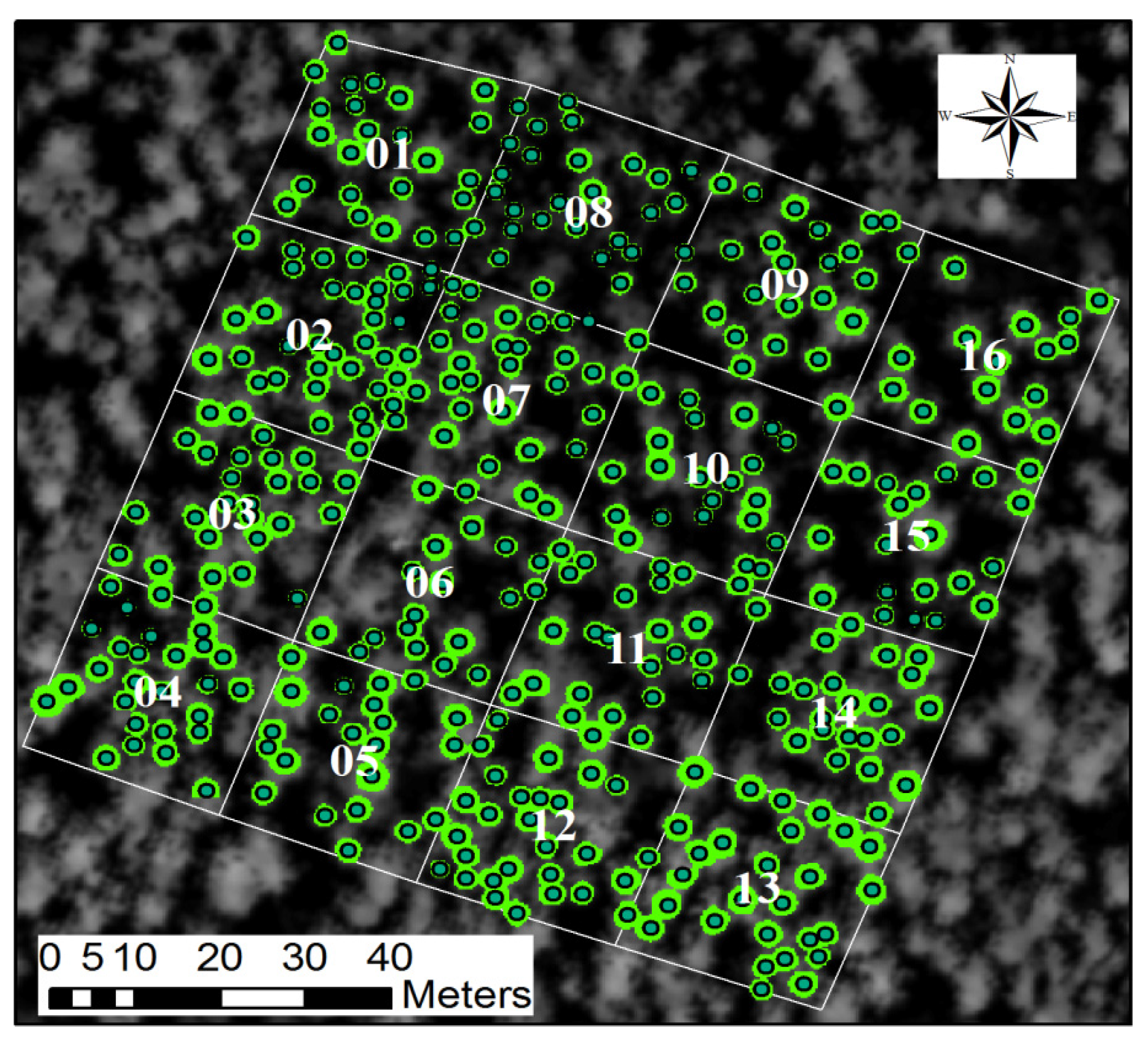
2.1. Study Site and Data

This study was conducted on the Xishui forest farm located in Su’nan Yuguzu Autonomous County, Dayekou Basin of Gansu Qilian Mountain National Nature Reserve, with longitudes and latitudes of 100°12’E to 100°20’E and 38°29’N to 38°35’N (Figure 1a). Its average elevation is 2993 m with a range of 2550–3680 m above mean sea level. The National Nature Reserve was established for water resource conservation in the temperate alpine cold semi-arid and semi-humid zone, which is mainly characterized by mountainous forests and steppe [26,27]. The forests are matured secondary pure natural forests with the ground covered by moss and mainly distributed in the shady slopes of this region, while the grass lands are typically found in the sunny slopes. The dominant species is Picea crassifolia Kom.

A representative forest stand of the entire Dayekou Basin of Gansu Qilian Mountain National Nature Reserve was selected to establish the permanent sample plot (PSP) of 100 m × 100 m along the hillside to properly represent forest stands with typical site conditions. The PSP was divided into 16 sub-sample plots of 25 m × 25 m (Figure 1c). The sub-sample plots within PSP were located using a DGPS (differential global position system) unit. Measurements for DBH, height (H), height to crown base, and crown width at two perpendicular directions were made for a total of 402 Picea crassifolia Kom trees with DBH larger than 5 cm. Trees were positioned using a total station as shown in Figure 1c.

A LiDAR LiteMapper 5600 system was utilized to collect point-cloud data on June 23 2008 [28]. The laser scanner called Riegl LMS-Q560 was used, which had a wavelength of 1550 nm with an interval of 3.5 nm, laser beam divergence of 0.5 mrad, pulse repetition frequency (PRF) of 50 kHz, maximum scanning angle of 30 degree, and scanning frequency of 49 Hz. The LiDAR data were collected at an average flying height of 3699 m and average flying speed of 230 km·h⁻¹. The spatial flight line configuration is shown in Figure 1b. The elevations of the point returns had a range of 2725 to 3193 m (Figure 2a) with an average point density of 4.34 points m⁻² (Figure 2b).

2.2. Estimating Tree Variables from LiDAR Imagery

In this study, stand-level variable SCD and individual tree-level variables, LH and CPA, were derived using the aforementioned LiDAR imagery. In the estimation of LH and CPA, tree crowns were first delineated based on point cloud data and a canopy height model (CHM) was created as the difference of the digital surface model (DSM) and digital elevation model (DEM). In order to generate the DSM that contains elevation information of the objects (such as trees) and ground features, the raw LiDAR point clouds were interpolated using the method of maximum height interpolation and null-cell filling with values of neighboring cells. Moreover, the DEM was derived using the last return LiDAR point clouds with a progressive morphological filter [29].

To derive CHM, determining an appropriate cell size of the grid would be critical [30]. The appropriate cell size was selected to reduce the number of raster gaps and preserve sufficient details. We used a grid cell size $c=\sqrt{n}$ based on the study of Chen et al. [30], where n was the pulse density; that is, the number of returns m⁻². Moreover, the Gaussian-smoothing filter was employed to mitigate noise in the data [31].

Theoretically, an image segmentation algorithm can be used to split CHM into different polygons. The polygon boundaries imply individual tree crowns, with the maximum of each polygon corresponding to the top of a tree. However, in this method, the gaps among the tree crowns are regarded as tree crowns, which leads to false crowns and an overestimation of crowns [32]. We used the local maxima algorithm [30] to create CHM. Using the local maxima algorithm, a potential crown top was first found for each tree and used as a seed point. Based on the seed point, the boundary of the tree crown was delineated using the regional growing method.

When the tree crown top was searched using the local maxima algorithm, the window size varied, which was determined from the correlations of tree height with crown width. Moreover, the window size was larger than or equal to the minimum crown width but smaller than or equal to the tree height [32,33]. In addition, delineation of the boundaries of tree crowns was carried out using the tangent value of the crown angle obtained with a crown angle recognition algorithm [32,33]. Many researchers have described this algorithm and the crown delineation approach in detail [32,34], and therefore are not discussed in this article. We delineated crowns for a total of 402 Picea crassifolia Kom trees in the 16 sub-sample plots nested in the PSP (Figure 3). A detailed description of the extraction method for SCD based on the airborne LiDAR point-cloud data was presented in Liu et al. [35]. Summary statistics of the tree-level information (LH and CPA) and stand-level information (SCD) are presented in

Table 1. Descriptive statistics of tree variable measurements (SD, standard deviation; DBH, diameter at breast height; LH, LiDAR-derived tree height; CPA, crown projection area; and SCD, stand canopy density).

Variable	Mean	SD	Min	Max
DBH (cm)	23.46	8.35	2.50	81.10
LH (m)	6.95	1.90	1.96	11.30
CPA (m2)	7.43	2.06	2.94	13.50
SCD	0.79	0.06	0.67	0.89

. Additionally, the corresponding statistics of ground-measured DBH are also presented in this table.

2.3. Nonlinear Mixed-Effects DBH Estimation Model

We formulated the individual tree DBH estimation models with sub-sample plot random effects following the NLME modeling technique:

$$DB{H}_{ij}=f({\mathit{\varphi }}_{ij},x_{ij})+{\epsilon }_{ij},\hspace{1em}i=1,\dots ,M,j=1,\dots ,n_i,$$

(1)

where $DB{H}_{ij}$ is the diameter at breast height of the j^th tree on the i^th sub- sample plot, $M$ is the number of sub-sample plots, $n_i$ is the number of observations in the i^th sub- sample plot, and $f(\cdot )$ is a real valued and differentiable function of a subject-specific parameter vector ${\mathit{\varphi }}_{ij}$ and a covariate vector $x_{ij}$. The within-group error vector ${\epsilon }_i={({\epsilon }_i,\dots ,{\epsilon }_{i{n}_i})}^T$ that accounts for within-group variance and correlation was assumed to follow a normal distribution with zero expectation and a positive-definite variance-covariance structure $R_i$ [36]. $R_i$ is expressed as a function of the parameter vector $\mathsf{\theta }$ [21]:

$${\epsilon }_i~N(0,R_i(\mathsf{\theta })).$$

(2)

Moreover, ${\mathit{\varphi }}_{ij}$ could be expressed as:

$${\mathit{\varphi }}_{ij}=A_{ij}\beta +B_{ij}{u}_i,u_i~N(0,\Psi ),$$

(3)

where $\beta$ is a p-dimensional vector of the fixed effects, $u_i$ is an independently and normally distributed $q$-dimensional vector of random effects with zero means and a variance-covariance matrix $\Psi$, $A_{ij}$ and $B_{ij}$ are design matrices, and $u_i$ and ${\epsilon }_{ij}$ are independent of each other.

2.4. Predictor Variables

Tree DBH could be related to two groups of relevant variables that were derived from LiDAR imageries, they are: Tree size variables (e.g., CPA and LH) and stand size variables (e.g., mean tree height and SCD). Existing methods and algorithms could be used to obtain tree variables with high accuracy [9,37]. To reduce the over-parameterization and collinearity effects, which leads to biased parameter estimation of the models, we selected only one stand-level variable: SCD, and two tree-level variables: CPA and LH as predictors to develop the DBH estimation models.

2.5. Base Model

Firstly, we considered four commonly used candidate models of various forms, including a linear model (Equation (4)), Richards model (Equation (5)), logistic model (Equation (6)), and exponential model (Equation (7)) as base models to fit the full data set (Table 1) with three predictor variables: SCD, CPA, and LH. Secondly, we chose the best performing one to develop the generalized NLME DBH estimation model through the inclusion of the random components describing the variations of DBH at the sub-sample plot level. All the models have four parameters, except Equation (6), which has five parameters:

$$DBH={\beta }_1+{\beta }_{2}LH+{\beta }_{3}CPA+{\beta }_{4}SCD+\epsilon ,$$

(4)

$$DBH={\beta }_1[1-\exp (-{\beta }_{2}LH-{\beta }_{3}CPA-{\beta }_{4}SCD)]+\epsilon ,$$

(5)

$$DBH={\beta }_1/[1+{\beta }_2\exp (-{\beta }_{3}LH-{\beta }_{4}CPA-{\beta }_{5}SCD)]+\epsilon ,$$

(6)

$$DBH={\beta }_1\exp (-{\beta }_{2}LH-{\beta }_{3}CPA-{\beta }_{4}SCD)+\epsilon ,$$

(7)

where ${\beta }_1-{\beta }_5$ are parameters and $\epsilon$ is an error term.

The best performing model selected based on the following statistical criteria [38] was used for further analyses:

$$\overline{e}={\displaystyle \sum e_t/N}={\displaystyle \sum (DB{H}_t-D\widehat{B}{H}_t})/N,$$

(8)

$$\delta ={\displaystyle \sum {(e_t-\overline{e})}^2/(N-1)},$$

(9)

$$R^2=1-\frac{{\displaystyle {\sum }_{t=1}^N{(DB{H}_t-D\widehat{B}{H}_t)}^2}}{{\displaystyle {\sum }_{t=1}^N{(DB{H}_t-D\overline{B}H)}^2}},$$

(10)

$$RMSE=\sqrt{{\overline{e}}^2+\delta },$$

(11)

where $DB{H}_t$ and $D\widehat{B}{H}_t$ are the observed and predicted diameter at breast height, respectively, of the $t^{th}$ tree; $D\overline{B}{H}_t$ is the mean of the observed DBH values; and $\overline{e}$, $\delta$, $R^2$, and RMSE are the mean bias, variance of bias, coefficient of determination, and root mean square error, respectively. The RMSE is defined as the combination of the mean bias and its variance. The RMSE is used as the most important evaluation criterion of the model. The nls function with OLS in R [39] was used for nonlinear regressions.

2.6. Parameter Effects

We used the best performing base model to develop a generalized NLME DBH estimation model with the sub-sample plot random effects included in it. All the NLME model alternatives were fitted to the full data set. The alternative models were formed with all possible combinations of the fixed-effects parameters with the random effects. The model variant with the smallest Akaike’s information criterion (AIC) and the largest log-likelihood (LL) was selected for further evaluation [40]. To avoid over-parameterization, the likelihood ratio test (LRT) was applied [41].

2.7. Determining the Structure of the Between Sub-Sample Plot Variance–Covariance Matrix ($\Psi$)

The variance–covariance matrix for the random effects at the sub-sample plot level, $\Psi$, which is common to all sub-sample plots, was assumed to account for the variability of DBH across these plots. $\Psi$ was assumed to be unstructured [42]. We assumed the $3\times 3$ variance-covariance matrix as shown below:

$$\left(\begin{array}{ccc}{\sigma }_{11}^2& {\rho }_{12}& {\rho }_{13}\\ {\rho }_{21}& {\sigma }_{22}^2& {\rho }_{23}\\ {\rho }_{31}& {\rho }_{32}& {\sigma }_{33}^2\end{array}\right),$$

where ${\sigma }_{ij}^2$($i,j=1,2,3,i=j$) is a variance in the i^th random effect and ${\rho }_{ij}$ ($i,j=1,2,3,i\ne j$) is a covariance of the i^th and j^th random effects.

2.8. Determining Structure of Within Sub-Sample Plot Variance–Covariance Matrix ($R$)

We applied the method suggested by Davidian and Giltinan [36] to account for within sub- sample plot heteroscedasticity and autocorrelation in the variance–covariance matrix ($R$) [21,36]:

$$R_i={\sigma }^2{G}_i^{0.5}{\Gamma }_i{G}_i^{0.5},$$

(12)

where ${\sigma }^2$ is an error dispersion, which is also known as a scaling factor and is equal to the residual variance of the model; $G_i$ is an $n_i\times n_i$ diagonal matrix of the within sub-sample plot heteroscedasticity variances; and ${\Gamma }_i$ is an $n_i\times n_i$ matrix of the within sub-sample plot autocorrelations. No pattern of autocorrelation emerged between the observations in our data; we therefore reduced ${\Gamma }_i$ to an $n_i\times n_i$ identity matrix.

We evaluated three commonly used variance-stabilizing functions: An exponential function Equation (13), a power function Equation (14) and a constant plus power function Equation (15) to account for the variance heterogeneity [15]. Then, the most effective variance function was chosen using the LRT and AIC [17,41]:

$$\mathrm{var}({\epsilon }_{ij})={\sigma }^2\exp (2\gamma x_{ij}),$$

(13)

$$\mathrm{var}({\epsilon }_{ij})={\sigma }^2{x}_{ij}{}^{2\gamma },$$

(14)

$$\mathrm{var}({\epsilon }_{ij})={\sigma }^2{({\gamma }_1+x_{ij}^{{\gamma }_2})}^2,$$

(15)

where $x_{ij}$ is a selected predictor ($LH$ and $CPA$); and $\gamma$, ${\gamma }_1$, and ${\gamma }_2$ are parameters to be estimated.

2.9. Model Estimation

The maximum likelihood with the Lindstrom and Bates (LB) algorithm implemented in the R software (version 3.4.2) nlme function [17,23] was used to estimate all NLME model variants. Many studies [17,23,43] have described the LB algorithm and nlme functions.

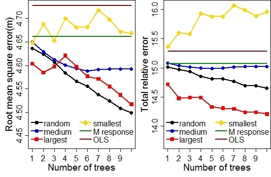
2.10. Subject-Specific Prediction

The NLME DBH estimation model was used to predict DBH with and without the random effects involved. A model becomes a mean response (M response) if the predicted random effects are not included, and a model with the predicted random effects becomes the subject-specific model or localized model. Localizing the mixed effects model is also known as calibration [21,44]. Calibration requires prior information of a response variable, i.e., DBH measurement from a sub-sample of trees in our case, for prediction. When no situation permits prediction of the random effects, either the M response or an OLS model (a model excluding the random effects on the fitting) needs to be used for DBH prediction. The empirical best linear unbiased prediction (EBLUP) theory [21,23] was used to predict the random effects:

$$\begin{gathered} {\widehat{u}}_i=\widehat{\Psi }{Z}_i^T{({\widehat{R}}_i+Z_i\widehat{\Psi }{Z}_i^T)}^{-1}{e}_i, \\ =\widehat{\Psi }{Z}_i^T{({\widehat{R}}_i+Z_i\widehat{\Psi }{Z}_i^T)}^{-1}\left[y_i-f(\widehat{\beta },u_i^{*},x_i)+Z_i{u}_i^{*}\right], \end{gathered}$$

(16)

where ${\widehat{u}}_i$ is a $q$- dimensional vector of the predicted random effects for the i^th sub-sample plot ($i=1,\dots ,M$); $u_i^{*}$ is a vector of EBLUP for random effects $u_i$; $f(\cdot )$ is an NLME DBH estimation model; $\widehat{\beta }$ is a vector of the estimated fixed-effect parameters $\beta$; $x_i$ is a vector of the predictors; $\widehat{\Psi }$ is an estimated variance-covariance matrix for the random effects $u_i$ ($i=1,\dots ,M$); ${\widehat{R}}_i$ is an estimated variance-covariance matrix for the error term $e_i$; $Z_i$ is an $n_i\times q$ dimensional design matrix of partial derivatives of NLME DBH estimation model $f(\cdot )$ with respect to random effects $u_i$. As the unknown random effects appeared on both sides of Equation (16), no direct algebraic solution for ${\widehat{u}}_i$ is possible. However, for its algebraic solution, Meng and Huang [21] developed a three-step iterative algorithm based on the EBLUP theory for the prediction of random effects. The computer program using R software for this algorithm was presented by Fu et al. [3].

We used DBH measurements from a varying number of sample trees for the prediction of the random effects in Equation (16). In general, the larger the number of sample trees used to localize the model, the higher the prediction accuracy [1,3,22]. Many modeling studies have determined the optimal number of sample trees necessary for the calibration of NLME models with reliable prediction accuracies. For example, studies have modelled the height–diameter relationships [1,40,45], basal area increment [40], diameter increment [42], and height to crown base [3]. Based on the previous studies by Calama and Montero [42] and Fu et al. [3], the following four alternatives were applied to select sample trees per sub-sample plot to account for the subject-specific variability of a response variable (DBH):

(i)

DBH of 1-10 randomly selected trees per sub-sample plot (random).

(ii)

DBH of 1-10 medium-size trees per sub-sample plot (medium).

(iii)

DBH of 1-10 the largest trees per sub-sample plot (largest).

(iv)

DBH of 1-10 the smallest trees per sub-sample plot (smallest).

Each sample of the trees selected for the four alternatives was repeated 100 times. The DBH estimates of the remaining trees on the same sub-sample plots were then obtained by computing the mean values of the corresponding tree’s DBH estimates according to the sampling results. We evaluated the prediction performances of each alternative with 1 to 10 sample trees using the full data set with the help of commonly used statistical measures, such as the root mean square error (RMSE) (Equation (11)) and total relative error (TRE) (Equation (17)):

$$TRE={\displaystyle \sum \left|DBH-D\widehat{B}H\right|}/{\displaystyle \sum D\widehat{B}H}.$$

(17)

2.11. Model Evaluation

The DBH estimation model could be validated using an independent data set. However, this was not possible in our study due to the small data set. Alternatively, we evaluated the predictive performance of DBH estimation models using the leave-one-out cross-validation (LOOCV) method [46,47], which is also feasible for a smaller data set. Data were naturally grouped by sub-sample plots. The LOOCV method was modified so that one sub-sample plot rather than a tree observation was left out from the full data set in each step and data from the left-out sub-sample plots were used to fit the DBH models. These models were then used to predict the DBH values of the trees within the deleted sub-sample plot. This was carried out for all 16 sub- sample plots in the full data set. The observed and predicted DBH values were then used to calculate some statistical measures of $\overline{e}$, $\delta$, $RMSE$, and $R^2$ (Equations (8)–(11)). The smaller the values of $\overline{e}$, $\delta$, and $RMSE$, and the larger the value of $R^2$, the higher the prediction accuracy of the models. The predictive performances of the NLME DBH estimation models, including their M responses and the corresponding base model, were compared based on the results of the LOOCV. The model with the smallest $\overline{e}$, $\delta$, and $RMSE$, and the largest $R^2$ was selected as a final DBH estimation model. The source codes for the LOOCV method employed in R version 3.4.2 are provided in Appendix A. We carried out all computations using R version 3.4.2.

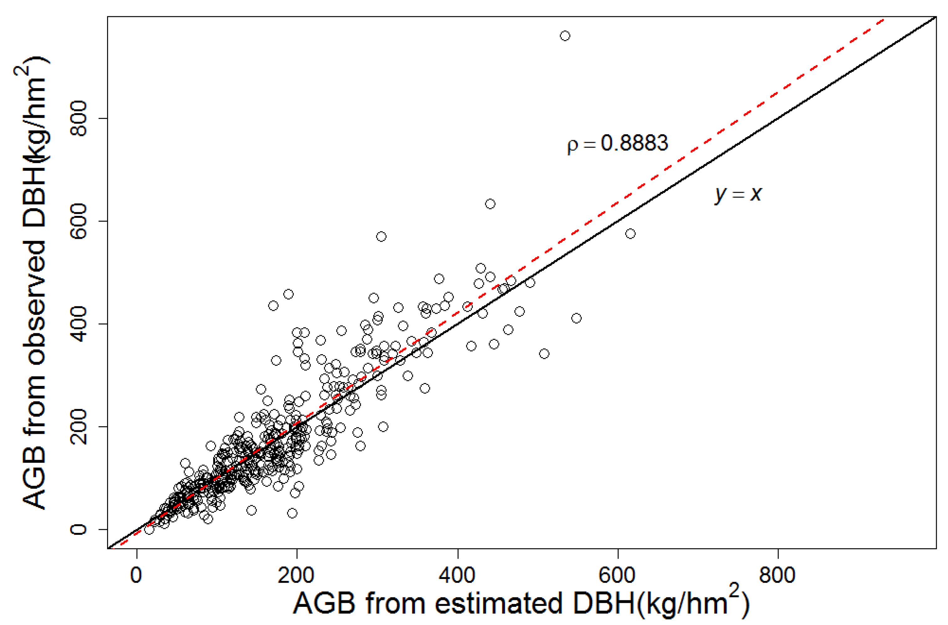
2.12. Model Application

The estimated forest biomass is useful for practical forestry and research [2]. The developed NLME DBH estimation model in this study can be used for estimating the biomass of each subject tree using the full data. Firstly, we estimated the DBH of 402 individual trees using the developed NLME DBH estimation model. Then, the biomasses of aboveground components (stem, branch, foliage, and fruit) of the 402 Picea crassifolia Kom trees were estimated using the empirical allometric models proposed by Wang et al. [48]. Finally, the aboveground biomass (AGB) of each subject tree was obtained by summing the component biomasses. The biomass of each subject tree obtained from both estimated DBH and observed DBH were evaluated using the Pearson correlation coefficient.

3. Results

3.1. Base Model

Both Equations (6) and (7) showed a slightly superior fitting performance compared to Equations (4) and (5) (

Table 2. Fit statistics of candidate base Equations (4)–(7) ($\overline{e}$, mean prediction error; $\delta$, variance of biases; $RMSE$, root mean square error; and $R^2$, coefficient of determination).

Models	$\overline{\mathit{e}}$	$\mathit{\delta }$	$\mathit{R}\mathit{M}\mathit{S}\mathit{E}$	${\mathit{R}}^2$
Model (4)	0.0000	4.8070	4.8070	0.6244
Model (5)	0.7426	4.9460	5.0010	0.5934
Model (6)	0.0040	4.7150	4.7150	0.6386
Model (7)	−0.0043	4.7190	4.7190	0.6381

). Relative to Equation (6), Equation (7) is more simplified with only four parameters, and it was therefore chosen as a basic nonlinear model to build the generalized NLME DBH estimation models based on the LiDAR-derived predictors. The estimated parameters for Equation (7) are listed in

Table 3. Parameter estimates and fit statistics of three different models (AIC, Akaike’s information criterion; and LL, log-likelihood).

	Parameters	Model (7)	Model (18)	Model (19)
Fixed-effects parameters	${\beta }_1$	12.90	16.64	15.98
	${\beta }_2$	−0.0954	−0.1141	−0.1083
	${\beta }_3$	−0.0458	−0.0346	−0.0372
	${\beta }_4$	0.5681	0.9495	0.8702
Variance components	$s_1$	-	0.2713	0.3543
	$s_2$	-	0.0020	0.0013
	$s_3$	-	0.0014	0.0152
	$s_{12}$	-	0.0124	0.0296
	$s_{13}$	-	−0.0058	0.0068
	$s_{23}$	-	−0.0230	0.0064
	$\gamma$	-	-	0.6189
	$\sigma$	4.7360	4.4150	4.3480
Model performance	AIC	2391	2382	2360
	−2LL	−1191	−1180	−1168

.

3.2. Generalized NLME DBH Estimation Model

Considering the four parameters in a model (${\beta }_1-{\beta }_4$), there were 15 different combinations of the random effects for the base Equation (7). All the NLME model alternatives converged with meaningful parameter estimates (omitted due to a limited space), but, the following NLME DBH estimation model (Equation (18)) exhibited the smallest AIC (2382) and the largest −2LL (−1180) among the converged models (Table 3):

$$DB{H}_{ij}=({\beta }_1+u_{1i})\exp \left[-({\beta }_2+u_{2i})L{H}_{ij}-({\beta }_3+u_{3i})CP{A}_{ij}-{\beta }_{4}SC{D}_i\right]+{\epsilon }_{ij},$$

(18)

where ${\beta }_1-{\beta }_4$ are the fixed effects parameters; and $u_{1i}$, $u_{2i}$, and $u_{3i}$ are random effects due to the $i^{th}$ sub-sample plot on ${\beta }_1-{\beta }_3$, respectively. The values of $u_i={(u_{1i},u_{2i},u_{3i})}^T$ varied with $i$, and $u_i$ were assumed to be distributed normally with zero expectation and a $3\times 3$ dimensional variance–covariance matrix of $\Psi$. For comparison, the within-group errors ${\epsilon }_{ij}$ were assumed to be independently normally distributed with homogeneous error variances. $u_i$ and ${\epsilon }_{ij}$ were assumed to have mutual independence. All other parameters and predictors are the same as defined earlier.

The parameter estimates of the NLME DBH estimation model (Equation (18)) are presented in Table 3. All the estimates were significant (p < 0.05). It was found that even with the random effects introduced, heteroskedasticity still existed in the DBH estimation model (Equation (18)) (Figure 5a). The empirical autocorrelation function for Equation (18) showed insignificant autocorrelations among the standardized residuals within the sample plots.

3.3. Parameter Estimation

We evaluated three variance-stabilizing functions, and the power variance function with LH as a predictor showed the best performance (

Table A1. Assessment of the nonlinear mixed-effects diameter at breast height model (18) with different variance functions (CPA, crown projection area (m²); LH, LiDAR derived tree height (m); AIC, Akaike’s information criterion; LL, log-likelihood; LR, likelihood ratio; EF, exponential function – Equation (13); PF, power function – Equation (14); CPF, constant plus power function – Equation (15); and variance function 1 meant that the variances were homogeneous).

Variance			CPA				LH
Function	AIC	−2LL	LR	p value	AIC	−2LL	LR	p value
1	2382	−1180			2382	−1180
PF	2363	−1169	21.56	<0.0001	2360	−1168	24.42	<0.0001
EF	2366	−1171	18.39	<0.0001	2361	−1169	22.87	<0.0001
CPF	2365	−1169	21.55	<0.0001	2362	−1168	24.42	<0.0001

), and therefore it was applied in Equation (18). All the estimates of Equation (18), with the power variance function included along with the evaluation metrics, are listed in Table 3. After substituting the estimated value of the fixed effects parameter into Equation (18), the final NLME DBH estimation model for Picea crassifolia Kom in western China would become:

$$DB{H}_{ij}=(15.98+u_{1i})\exp \left[-(-0.1083+u_{2i})L{H}_{ij}-(-0.0372+u_{3i})CP{A}_{ij}-0.8702SC{D}_i\right]+{\epsilon }_{ij}$$

(19)

where:

• $u_i=\left[\begin{array}{l}{u}_{1i}\\ u_{2i}\\ u_{3i}\end{array}\right]~N\left\{\left[\begin{array}{l}0\\ 0\\ 0\end{array}\right],{\Psi }_1=\left(\begin{array}{ccc}0.3543& 0.0296& 0.0068\\ 0.0296& 0.0013& 0.0064\\ 0.0068& 0.0064& 0.0152\end{array}\right)\right\}$,
• ${\epsilon }_i={({\epsilon }_{i1},\dots ,{\epsilon }_{i{n}_i})}^T~N\left(0,R_i=18.91G_i^{0.5}{\Gamma }_i{G}_i^{0.5}\right)$,
• $G_i=diag\left(L{H}_{i1}{}^{1.238},\dots ,L{H}_{i{n}_i}{}^{1.238}\right)$,
• ${\Gamma }_i=I_{n_i}$,
• and $I_{n_i}$ was an $n_i\times n_i$ identity matrix. All other parameters and predictors in this model are the same as defined earlier.

Equation (19) led to a smaller AIC and larger LL values than both Equations (7) and (18) with homogeneous error variances, indicating that the sample sub-sample plot exerted significant random effects on the predictions of DBH.

3.4. Subject-Specific DBH Prediction

The patterns of the prediction statistics for a calibrated response with different sampling strategies are shown in Figure 4. Both the $RMSE$ and $TRE$ for four sampling strategies had similar trends. Regardless of the number of trees (1 to 10 trees) for each sampling strategy, except the smallest trees used for calibration of the model or its localization at the sample plot level, both $RMSE$ and $TRE$ for Equation (19) were smaller than that of the M response and OLS Equation (7). Calibration of Equation (19) with the alternatives of the randomly selected trees and largest trees showed a steadily increasing accuracy of DBH when a larger number of trees were used for the random effect predictions. When the largest tree per sub-sample plots were used in the calibration, Equation (19) produced the smallest $TRE$. The model $RMSE$ did not follow the same trends. With the selection of two or fewer sample trees, the $RMSE$ for the largest trees is smaller than that for randomly selected trees. When the selection of more than two sample trees, the $RMSE$ for the largest trees is larger than that for randomly selected trees. Figure 4 also shows the greatest reduction rates in the $RMSE$ and $TRE$ of Equation (19) when the two largest trees were used in the calibration. This led to the reduction of the $RMSE$ and $TRE$ by 3.4% and 3.9%, respectively, compared to that of the M response. The $RMSE$ and $TRE$ could be further reduced by selecting a larger number of the largest trees in the calibration. However, the inclusion of several sample trees could increase the inventory cost. Using only the two largest trees per sub-sample plot for the calibration could provide the most cost-effective and accurate predictions of Equation (19). Calibration of the mixed-effects model using only an optimal number of sample trees with a high prediction accuracy is always a better strategy for efficient forest management.

3.5. Model Evaluation

The prediction statistics based on the cross-validation method for Equation (7) and Equation (19) in two cases, at the M response and sub-sample plot level, are presented in

Table 4. Prediction statistics of two models using the leave-one sub-sample plot-out cross-validation ($\overline{e}$, mean prediction error; $\delta$, variance of biases; $RMSE$, root mean square error; $R^2$, coefficient of determination; and M response, mean response).

Model	$\overline{\mathit{e}}$	$\mathit{\delta }$	$\mathit{R}\mathit{M}\mathit{S}\mathit{E}$	${\mathit{R}}^2$
Model (7)	0.1101	4.6530	4.7280	0.6122
Model (19)
M response	0.0843	4.6570	4.6620	0.6335
Sub-sample plot level	−0.0307	4.4210	4.4210	0.6815

. The mean prediction biases for these models were not significant (p < 0.05).

The $\delta$ and $RMSE$ of Equation (19) were much smaller, and the $R^2$ value was much larger than its counterparts for Equation (19) at the M response and Equation (7). This indicated that the estimated random effects at the sub-sample plot-level on the prediction of DBH were large and their introduction substantially improved the model’s prediction accuracy. Among these models, Equation (19) at the sub-sample plot level showed the highest prediction accuracy of DBH. For example, Equation (19) at the sub-sample plot level resulted in an $RMSE$ of 4.4210, which was 5.2% and 6.5% smaller than those of Equation (19) at the M response and Equation (7), respectively. Moreover, Equation (19) at the sub-sample plot level resulted in an $R^2$ of 0.6815 and the increases of 7.6% and 11.3% compared to that of Equation (19) at the M response and Equation (7), respectively. Therefore, Equation (19) was recommended to predict individual tree DBH based on the LiDAR data.

Figure 5b shows the residuals distribution of the NLME DBH estimation model (Equation (19)) at the sub-sample plot level based on the leave-one sub-sample plot-out cross-validation. Compared to Equation (18) with homogeneous error variances (Figure 5a), heteroscedasticity was significantly reduced for Equation (19). This showed that the power variance function applied with LH as a predictor effectively accounted for heteroscedasticity (Figure 5b).

3.6. Model Application

Based on the above-mentioned Equations (19) and provisions, the estimated DBH of all subject trees were used for estimating their corresponding AGB. Figure 6 shows the scatter plots of the predicted AGB from the observed DBH against that from the estimated DBH by Equation (19). This figure confirmed that the two sets of AGB estimates were very close and the corresponding Pearson correlation coefficient of the two sets of AGB estimates was 0.89. This suggested that the presented NLME DBH estimation model could be used for a precise estimation of AGB, and is thus important for informed decision-making in forestry.

4. Discussion

This study established the generalized tree-based NLME DBH model to predict DBH of Picea crassifolia Kom trees in western China. The sub-sample plot variability was included in the model through modeling of the random effects that were specific to the sub-sample plot. The NLME modeling also allowed the dependent observations obtained from the nested data structure to be dealt with. Additionally, when using the random component models, we considered the unique variance-covariance structure for the individual tree DBH estimation model to which a random part indicating a sub-sample plot deviation from the mean behavior was also added. Deviation values could be properly explained by tree- and stand-level variables and their integration [3,18].

The CPA and LH could be estimated using airborne LiDAR data and used to infer DBH based on the model (Equation (19)). Previous studies [2,49] have proved that DBH is the most reliable measurable tree variable for biomass estimation. Therefore, DBH offers a useful tool for remote sensing techniques for assessment of the aboveground biomass over the extensive forest area. Several researchers [50,51] have also reported that some variables, such as crown diameter and crown volume, have significant contributions to the prediction accuracy of DBH. We evaluated these variables for their potential contributions to improve the model; however, the prediction accuracy of Equation (19) was not significantly improved when crown diameter or crown volume was included. This insignificant contribution probably resulted from the collinearity between these crown characteristics and CPA. Based on the rapidly advancing remote sensing technology, CPA can be more easily measured than crown diameter; this is because the derived crown diameter could be influenced by measurement directions [52]. To mitigate the uncertainty from the crown diameter measurement, CPA was used in our modeling.

Calibration of the mixed-effects models using a small number of sample trees is the most useful in forestry application [3,21]. All those tree- and stand-level variables, which could have significant effects on the DBH, cannot be directly measured in routine inventories. The effects of such variables may be captured indirectly by a small number of sample trees per sample plot that are used to calibrate the mixed-effects models, and this would result in a great improvement on the model’s prediction accuracy [3]. We found remarkably better calibration results were achieved from the two largest trees per sample plot that were used to predict the sample’s plot-level random effects. For the smallest trees, the calibration results were the worst. For example, calibration with the inclusion of the random effects increases the prediction accuracy of the NLME DBH models even when the EBLUP theory is applied based on the largest tree per sub-sample plot (Figure 4), but the smallest trees failed to do so. This indicates that only the largest trees could effectively describe the random effects of the sub-sample plot, especially for LiDAR data. This is probably because the largest trees are usually considered as dominant trees in the sub-sample plot. Their heights, also defined as dominant heights, are used to reflect the stand and tree developments and the dominant height is also a reliable indicator of site productivity, and therefore it is frequently used in different forest models [3,53].

The estimated random effects using a large number of sample trees for calibration of the NLME DBH model is not often justifiable, as this increases sampling and measurement cost [3]. The evaluation of 10 different sample sizes (from 1 to 10 trees) for the four alternatives used in calibration showed a higher prediction accuracy with an increased number of sample trees (Figure 4). This result is consistent with the results, for example, from the studies modeling height–diameter relationships [18,45,54] and individual tree height to crown base [3]. The model calibrated using the two largest trees per sub-sample plot could also result in the most accurate prediction with a reasonably low sampling and measurement cost. Calibration of the mixed-effects model using only a reasonable number of sample trees with a great accuracy is always a better alternative for efficient forest management. Thus, the two largest trees per sub-sample plot, which are assumed to balance the sampling cost and potential errors of the prediction, can be recommended as an optimal sample size for DBH prediction with high accuracy. It should be noted that Equation (19) at the M response might be used when the prediction accuracy of DBH is not a concerning issue in the model application. When prior information of a response variable (DBH) is not available, the M response can be used. With reference to the base Equation (7), the accuracy of Equation (19) at the M response was significantly improved (Table 4). For example, the $RMSE$ and $R^2$ values from Equation (19) at the M response were 4.662 and 0.6335, which were 1.4% smaller and 3.5% larger than those of the base Equation (7), respectively.

Unlike the conventional ground-based methods, the DBH estimation models developed from the remote sensing data could be used for a large-scale assessment of aboveground forest biomass. The empirical models built using any data set may be applicable for predicting the response variable in other data sets that are different from the modeling data [55]. Thus, the NLME modeling approach is employed to estimate DBH from LiDAR imagery, not only in situations in which the imagery feature is captured, but the features of the forest stands should also be taken into account.

There could be some important challenges while modeling DBH using both ground- and LiDAR-based datasets. For example, the estimates of CPA and LH are subject to errors, although the measurements of any tree variables are generally assumed to be free of significant errors [55]. The omission and commission errors that occur in the crown delineation are another challenge [12,13,55]. The measurement errors arising due to imagery illuminations, delineation algorithms, and geometric features of the crown shape on the imageries can be substantial [55]. Especially, the delineation algorithms are very sensitive to forest stand density. In all the existing DBH estimation models [5,6,7,8], including that developed in our study (e.g., Equation (19)), DBH is assumed as a random variable and all predictor variables are fixed and observed without errors. The fact is that the violation of the second assumption may lead to biased parameter estimates and their variances and consequently, mislead the hypothesis tests [55]. If the predictors in Equation (19) are assumed to have significant errors, alternatively, any new NLME modeling approach is necessary to deal with such error problems. However, none of the algorithms and computational techniques are available so far to implement such a new approach. This article emphasizes more on the methodology for a natural pure forest, and it may be useful for other researchers to develop similar NLME DBH models using a remotely sensed database of other species as well. For natural mixed forests, we are also in the process of developing models using the NLME modeling approach to estimate individual tree DBH based on airborne LiDAR data.

5. Conclusions

We developed a generalized nonlinear mixed-effects DBH estimation model for Picea crassifolia Kom trees in western China. Data acquired from the Airborne LiDAR LiteMapper 5600 system with a high spatial resolution were used to estimate stand canopy density, crown projection area, and tree height, which were involved in the DBH estimation model as predictors. The random effects of the sub-sample plots on the DBH variations were significant, and the introduction of these effects into the model resulted in a substantial improvement of the DBH prediction accuracy. The heteroskedasticity problem was substantially reduced by introducing the power variance function with tree height as a predictor. Relative to the base model, the prediction accuracy of the generalized nonlinear mixed-effects model at the mean response was also significantly increased. Calibration of the mixed-effects DBH estimation model using the two largest sample trees per sub-sample plot provided a reasonably higher accuracy compared to other alternatives. This sample size is therefore considered suitable for estimating random effects, as this alternative is assumed to balance both measurement cost and potential prediction errors. The nonlinear mixed-effects DBH estimation at the mean response can be applied if obtaining the values of individual tree DBH, with a relatively lower cost and lower prediction accuracy being the purpose of the study.

References

1. Crecente-Campo, F.; Tomé, M.; Soares, P.; Dieguez-Aranda, U. A generalized nonlinear mixed-effects height-diameter model for Eucalyptus globulus L. in northwestern Spain. For. Ecol. Manag. 2010, 259, 943–952. [Google Scholar] [CrossRef] [Green Version]
2. Fu, L.; Lei, Y.; Wang, G.; Bi, H.; Tang, S.; Song, X. Comparison of seemingly unrelated regressions with multivariate errors-in-variables models for developing a system of nonlinear additive biomass equations. Trees 2016, 30, 839–857. [Google Scholar] [CrossRef]
3. Fu, L.; Zhang, H.; Sharma, R.P.; Pang, L.; Wang, G. A generalized nonlinear mixed-effects height to crown base model for Mongolian oak in northeast China. For. Ecol. Manag. 2017, 384, 34–43. [Google Scholar] [CrossRef]
4. Fu, L.; Sharma, R.P.; Hao, K.; Tang, S. A generalized interregionalnonlinear mixed-effects crown width model for Prince Rupprecht larch in northern China. For. Ecol. Manag. 2017, 384, 34–43. [Google Scholar] [CrossRef]
5. Popescu, S.C. Estimating biomass of individual pine trees using airborne lidar. Biomass Bioenerg. 2007, 31, 646–655. [Google Scholar] [CrossRef]
6. Broadbent, E.N.; Asner, G.P.; Peña-Claros, M.; Palace, M.; Soriano, M. Spatial partitioning of biomass and diversity in a lowland Bolivian forest: Linking field and remote sensing measurements. For. Ecol. Manag. 2008, 255, 2602–2616. [Google Scholar] [CrossRef]
7. Heurich, M. Automatic recognition and measurement of single trees based on data from airborne laser scanning over the richly structured natural forests of the Bavarian Forest National Park. For. Ecol. Manag. 2008, 255, 2416–2433. [Google Scholar] [CrossRef]
8. Bi, H.; Fox, J.C.; Li, Y.; Lei, Y.; Pang, Y. Evaluation of nonlinear equations for predicting diameter from tree height. Can. J. For. Res. 2012, 42, 789–806. [Google Scholar] [CrossRef]
9. Andersen, H.E.; Reutebuch, S.E.; McGaughey, R.J. A rigorous assessment of tree height measurements obtained using airborne lidar and conventional field methods. Can. J. Remote Sens. 2006, 32, 355–366. [Google Scholar] [CrossRef]
10. Gatziolis, D.; Fried, J.S.; Monleon, V.S. Challenges to estimating tree height via LiDAR in closed-canopy forests: A parable from western Oregon. For. Sci. 2010, 56, 139–155. [Google Scholar]
11. Vauhkonen, J.; Mehtätalo, L.; Packalén, P. Combining tree height samples produced by airborne laser scanning and stand management records to estimate plot volume in Eucalyptus plantations. Can. J. For. Res. 2011, 41, 1649–1658. [Google Scholar] [CrossRef]
12. Duncanson, L.; Cook, B.; Hurtt, G.; Dubayah, R. An efficient, multi-layered crown delineation algorithm for mapping individual tree structure across multiple ecosystems. Remote Sens. Environ. 2014, 154, 378–386. [Google Scholar] [CrossRef]
13. Aubry-Kientz, M.; Dutrieux, R.; Ferraz, A.; Saatchi, S.; Hamraz, H.; Williams, J.; Coomes, D.; Piboule, A.; Vincent, G. A Comparative Assessment of the Performance of Individual Tree Crowns Delineation Algorithms from ALS Data in Tropical Forests. Remote Sens. 2019, 11, 1086. [Google Scholar] [CrossRef] [Green Version]
14. Moore, J.R. Allometric equations to predict the total aboveground biomass of radiata pine trees. Ann. For. Sci. 2010, 67, 806. [Google Scholar] [CrossRef] [Green Version]
15. Rombouts, J.; Ferguson, I.S.; Leech, J.W. Campaign and site effects in LiDAR prediction models for site-quality assessment of radiata pine plantations in South Australia. Int. J. Remote Sens. 2010, 31, 1155–1173. [Google Scholar] [CrossRef]
16. Herrera-Fernández, J.J.; Campos, J.J.; Kleinn, C. Site productivity estimation using height-diameter relationships in Costa Rican secondary forests. For. Syst. 2004, 13, 295–303. [Google Scholar]
17. Pinheiro, J.C.; Bates, D.M. Mixed-Effects Models in S and S-PLUS; Springer: New York, NY, USA, 2000. [Google Scholar]
18. Calama, R.; Montero, G. Interregional nonlinear height-diameter model with random coefficients for stone pine in Spain. Can. J. For. Res. 2004, 34, 150–163. [Google Scholar] [CrossRef] [Green Version]
19. Schabenberger, O.; Gregoire, T.G. A conspectus on estimating function theory and its application to recurrent modelling issues in forest biometry. Silva Fenn. 1995, 29, 49–70. [Google Scholar] [CrossRef] [Green Version]
20. West, P.W.; Ratkowsky, D.A.; Davis, A.W. Problems of hypothesis testing of regressions with multiple measurements from individual sampling units. For. Ecol. Manag. 1984, 7, 207–224. [Google Scholar] [CrossRef]
21. Meng, S.X.; Huang, S. Improved calibration of nonlinear mixed-effects models demonstrated on a height growth function. For. Sci. 2009, 55, 239–248. [Google Scholar]
22. Fu, L.; Sun, H.; Sharma, R.P.; Lei, Y.; Zhang, H.; Tang, S. Nonlinear mixed-effects crown width models for individual trees of Chinese fir (Cunninghamia lanceolata) in south-central China. For. Ecol. Manag. 2013, 302, 210–220. [Google Scholar] [CrossRef]
23. Lindstrom, M.J.; Bates, D.M. Nonlinear mixed effects models for repeated measures data. Biometrics 1990, 46, 673–687. [Google Scholar] [CrossRef] [PubMed]
24. Vonesh, E.F.; Chinchilli, V.M. Linear and Nonlinear Models for the Analysis of Repeated Measurements; Marcel Dekker: New York, NY, USA, 1997. [Google Scholar]
25. Adame, P.; Río, M.D.; Cañellas, I. A mixed nonlinear height diameter model for Pyrenean oak (Quercus pyrenaica Willd.). For. Ecol. Manag. 2008, 256, 88–98. [Google Scholar] [CrossRef]
26. Dang, H.Z.; Zhao, Y.S.; Chen, X.W. Law of the water transfer process of water—Conversation forest in Qilian Mountains. Chin. J. Eco-Agric. 2004, 12, 43–46. [Google Scholar]
27. Ma, Y.J.; Wang, J.Y.; Liu, X.M.; Pei, W.; Jin, M. Status of Forestry Ecosystem and Protection Countermeasure in the Protection Areas in Qilian Mountains. J. Northwest For. 2005, 20, 5–8. [Google Scholar]
28. Pang, Y.; Chen, E.; Liu, Q.; Xiao, Q.; Zhong, K.; Li, X.; Ma, M. WATER: Dataset of airborne LiDAR mission at the super site in the Dayekou watershed flight zone on Jun. 23, 2008. In Chinese Academy of Forestry; Institute of Remote Sensing Applications, Chinese Academy of Sciences; Cold and Arid Regions Environmental and Engineering Research Institute, Chinese Academy of Sciences; Heihe Plan Science Data Center: Lanzhou, China, 2008. [Google Scholar] [CrossRef]
29. Zhang, K.; Chen, S.C.; Whitman, D.; Shyu, M.L.; Yan, J.; Zhang, C. Aprogressive morphological filter for removing nonground measurements fromairborne LIDAR data. IEEE Trans. Geosci. Remote Sens. 2003, 41, 872–882. [Google Scholar] [CrossRef] [Green Version]
30. Chen, Q.; Baldocchi, D.; Gong, P.; Kelly, M. Isolating individual trees in asavanna Woodland using small footprint lidar data. Photogramm. Eng. Remote Sens. 2006, 72, 923–932. [Google Scholar] [CrossRef] [Green Version]
31. Wu, B.; Yu, B.; Huang, C.; Wu, Q.; Wu, J. Automated extraction of groundsurface along urban roads from mobile laser scanning point clouds. Remote Sens. Lett. 2016, 7, 170–179. [Google Scholar] [CrossRef]
32. Liu, Q. Study on the Estimation Method of Forest Parameters Using Airborne LiDAR. Ph.D. Dissertation, Chinese Academy of Forestry, Beijing, China, 2009. [Google Scholar]
33. Koch, B.; Heyder, U.; Weinacker, H. Detection of Individual Tree Crowns in Airborne Lidar Data. Photogramm. Eng. Remote Sens. 2006, 72, 357–363. [Google Scholar] [CrossRef] [Green Version]
34. Liu, Q.; Li, Z.; Chen, E.; Pang, Y.; Wu, H. Extracting individual tree heights and crowns using airborne LIDAR data. J. Beijing For. Univ. 2008, 30, 83–89. [Google Scholar]
35. Liu, Q.; Fu, L.; Wang, G.; Li, S.; Li, Z.; Chen, E.; Pang, Y.; Hu, K. Improving Estimation of Forest Canopy Cover by Introducing Loss Ratio of Laser Pulses Using Airborne LiDAR. IEEE Trans. Geosci. Remote 2019, 58, 567–585. [Google Scholar] [CrossRef]
36. Davidian, M.; Giltinan, D.M. Nonlinear Models for Repeated Measurement Data; Chapmanand Hall: New York, NY, USA, 1995. [Google Scholar]
37. Nilsson, M. Estimation of tree heights and stand volume using an airborne lidar system. Remote Sens. Environ. 1996, 56, 1–7. [Google Scholar] [CrossRef]
38. Huuskonen, S.; Miina, J. Stand-level growth models for young scots pine stands in Finland. For. Ecol. Manag. 2007, 241, 49–61. [Google Scholar] [CrossRef]
39. Venables, W.N.; Ripley, B.D. Modern Applied Statistics with S-PLUS, 3rd ed.; Springer: New York, NY, USA, 1999. [Google Scholar]
40. Yang, Y.; Huang, S.; Meng, S.X.; Trincado, G.; VanderSchaaf, C.L. A multilevel individual tree basal area increment model for aspen in boreal mixedwood stands. Can. J. For. Res. 2009, 39, 2203–2214. [Google Scholar] [CrossRef]
41. Fang, Z.; Bailey, R.L. Nonlinear mixed-effect modeling for Slash pine dominant height growth following intensive silvicultural treatments. For. Sci. 2001, 47, 287–300. [Google Scholar]
42. Calama, R.; Montero, G. Multilevel linear mixed model for tree diameter increment in stone pine (pinus pinea): A calibrating approach. Silva Fenn. 2005, 39, 37–54. [Google Scholar] [CrossRef] [Green Version]
43. Tang, S.Z.; Li, Y.; Fu, L.Y. Statistical Foundation for Biomathematical Models, 2nd ed.; Higher Education Press: Beijing, China, 2015. [Google Scholar]
44. De-Miguel, S.; Mehtätalo, L.; Shater, Z.; Kraid, B.; Pukkala, T. Evaluating marginal and conditional predictions of taper models in the absence of calibration data. Can. J. For. Res. 2012, 42, 1383–1394. [Google Scholar] [CrossRef]
45. Temesgen, H.; Monleon, V.J.; Hann, D.W. Analysis and comparison of nonlinear tree height prediction strategies for Douglas-fir forests. Can. J. For. Res. 2008, 38, 553–565. [Google Scholar] [CrossRef] [Green Version]
46. Nord-Larsen, T.; Meilby, H.; Skovsgaard, J.P. Site-specific height growth models for six common tree species in Denmark. Scand. J. For. Res. 2009, 24, 194–204. [Google Scholar] [CrossRef]
47. Timilsina, N.; Staudhammer, C.L. Individual tree-based diameter growth model of slash pine in Florida using nonlinear mixed modeling. For. Sci. 2013, 59, 27–31. [Google Scholar] [CrossRef]
48. Wang, J.Y.; Ju, K.J.; Fu, H.E.; Chang, X.X.; He, H.Y. Study on biomass of water conservation forest on North Slope of Qilian Mountains. J. Fujian Coll. For. 1998, 18, 319–325. [Google Scholar]
49. Zeng, W.S.; Zhang, H.R.; Tang, S.Z. Using the dummy variable model approach to construct compatible single-tree biomass equations at different scales—A case study for Masson pine (Pinus massoniana) in southern China. Can. J. For. Res. 2011, 41, 1547–1554. [Google Scholar] [CrossRef]
50. Hall, R.J.; Morton, R.T.; Nesby, R.N. A Comparison of existing models for DBH estimation for large-scale photos. For. Chron. 1989, 65, 114–116. [Google Scholar] [CrossRef] [Green Version]
51. Gering, L.R.; May, D.M. The relationship of diameter at breast height and crown diameter for four species groups in Hardin county, Tennessee. South. J. Appl. For. 1995, 19, 177–181. [Google Scholar] [CrossRef] [Green Version]
52. Verma, N.K.; Lamb, D.W.; Reid, N.; Wilson, B. An allometric model for estimating DBH of isolated and clustered Eucalyptus trees from measurements of crown projection area. For. Ecol. Manag. 2014, 326, 125–132. [Google Scholar] [CrossRef]
53. Fu, L.; Sharma, R.P.; Zhu, G.; Li, H.; Hong, L.; Guo, H.; Duan, G.; Shen, C.; Lei, Y.; Li, Y.; et al. Comparing height–age and height–diameter modelling approaches for estimating site productivity of natural uneven-aged forests. Forestry 2018, 91, 419–433. [Google Scholar] [CrossRef]
54. Castedo-Dorado, F.C.; Diéguez-Aranda, U.; Anta, M.B.; Rodríguez, M.S.; Gadow, K.V. A generalized height-diameter model including random components for radiate pine plantations in northwestern Spain. For. Ecol. Manag. 2006, 229, 202–213. [Google Scholar] [CrossRef]
55. Zhang, W.; Ke, Y.; Quackenbush, L.J.; Zhang, L. Using error-in-variable regression to predict tree diameter and crown width from remotely sensed imagery. Can. J. For. Res. 2010, 40, 1095–1108. [Google Scholar] [CrossRef]
Figure 1. (a) Location of the study site: Xishui forest farm located in Su’nan Yuguzu Autonomous County of the Gansu Qilian Mountains National Nature Reserve, Western China; (b) spatial distribution of flight lines on orthorectified charge-coupled device images (WGS1984 UTM Zone 47N); and (c) tree positions within 16 sub-sample plots within a permanent sample plot of 100 m × 100 m.
Remotesensing 12 01066 g001
Figure 2. Spatial distribution patterns of the elevation (a) and density of laser points (b) on the study site.
Remotesensing 12 01066 g002
Figure 3. The spatial distribution of 402 tree crowns in 16 sub-sample plots nested in a permanent sample plot.
Remotesensing 12 01066 g003
Figure 4. Root mean squared error (RMSE) for ordinary least square (OLS) Equation (7), Equation (19) with mean response (M response), and Equation (19) calibrated with four sampling strategies and sample sizes for diameter at breast height within each sub-sample plot, for estimating the random effects (random: randomly selected trees; largest: the largest trees; medium: medium-size trees; and smallest: the smallest trees).
Remotesensing 12 01066 g004
Figure 5. Prediction errors based on Equation (18) with a variance-stabilizing function excluded (a) and prediction errors based on Equation (19) (b) with a variance-stabilizing function included
Remotesensing 12 01066 g005
Figure 6. Scatter plots of the predicted aboveground biomass (AGB) from the observed diameter at breast height (DBH) against that from the estimated DBH by Equation (19), with the red dotted line illustrating a linear relationship between two variables, black line denoting y = x , ρ is the correlation coefficient of the predicted AGB from the estimated DBH by Equation (19) and the observed DBH.
Remotesensing 12 01066 g006