Multi-Label Learning based Semi-Global Matching Forest

Abstract

Semi-Global Matching (SGM) approximates a 2D Markov Random Field (MRF) via multiple 1D scanline optimizations, which serves as a good trade-off between accuracy and efficiency in dense matching. Nevertheless, the performance is limited due to the simple summation of the aggregated costs from all 1D scanline optimizations for the final disparity estimation. SGM-Forest improves the performance of SGM by training a random forest to predict the best scanline according to each scanline’s disparity proposal. The disparity estimated by the best scanline acts as reference to adaptively adopt close proposals for further post-processing. However, in many cases more than one scanline is capable of providing a good prediction. Training the random forest with only one scanline labeled may limit or even confuse the learning procedure when other scanlines can offer similar contributions. In this paper, we propose a multi-label classification strategy to further improve SGM-Forest. Each training sample is allowed to be described by multiple labels (or zero label) if more than one (or none) scanline gives a proper prediction. We test the proposed method on stereo matching datasets, from Middlebury, ETH3D, EuroSDR image matching benchmark, and the 2019 IEEE GRSS data fusion contest. The result indicates that under the framework of SGM-Forest, the multi-label strategy outperforms the single-label scheme consistently.

1. Introduction

Dense matching recovers depth information from the dense correspondence between stereo imagery. Focusing on the similarity of patches to locate corresponding points is the most intuitive strategy (local stereo methods) and requires less computational effort [1]. The performance, however, is not competitive with methods considering spatial smoothness simultaneously (global stereo methods) at the cost of efficiency [1]. Semi-Global Matching (SGM) provides a good trade-off between accuracy and efficiency [2,3,4,5]. It regularizes disparity estimation by performing 1D Scanline Optimization (SO) [6] in multiple canonical directions, typically 8 or 16, and then summing up the corresponding energy functions. Thus, 2D SO is approximated and the disparity value corresponding to the minimum energy is selected based on the winner-take-all (WTA) strategy.

SGM has been applied in numerous fields, including building reconstruction, digital surface model generation, robot navigation, driver assistance and so forth [7,8,9]. However, the energy summation from all scanlines and the corresponding WTA strategy are empirical steps without a theoretical background, which is essentially inadequate when different scanlines propose inconsistent solutions [10]. Schönberger et al. [10] proposed SGM-Forest, which trained a random forest to predict a scanline with the best disparity proposal. Accordingly, a confidence value is obtained for each scanline, allowing for a confidence-based weighted average of the corresponding disparity prediction to refine the result. The algorithm is robust and performs steadily better than standard SGM in multiple stereo matching benchmark datasets [11,12].

However, in practice, there can be more than one scanline with good disparity prediction. It appears when multiple scanlines properly perceive the scene structure, therefore, are capable of predicting accurate disparity values simultaneously. For example, on a slanted plane extending horizontally, the two vertical scanlines (from bottom to top, and inversely), along which the slope is not explicitly expressed, should have better disparity estimation than the horizontal ones but achieve similar performance. Thus, the random forest gets confused when only a single best has to be selected.

In our project, we define a standard to determine good or bad scanlines, aiming at guiding the random forest to select as many good scanlines as possible for disparity prediction. The samples with zero scanline selection (all regarded as bad) are included for training, so that a more comprehensive prediction is obtained. The structure of the paper is as follows: Firstly, related work for improving SGM is described in Section 2. Afterwards, the standard SGM and SGM-Forest are recapped in Section 3, followed by our extension of SGM-Forest based on multi-label classification. In Section 4, the methods are tested on two close-range stereo matching datasets, Middlebury and ETH3D benchmarks [12,13,14,15], an airborne dataset, EuroSDR image matching benchmark [16], and a satellite dataset from the 2019 IEEE GRSS data fusion contest [17,18]. The comparison is recorded between original SGM-Forest based on single-label classification (termed SGM-ForestS for the follow-up) and our proposed implementation based on multi-label classification (termed SGM-ForestM). The results indicate higher performance of the latter. Finally, the conclusion is drawn in Section 5 with an outlook for future work.

2. Related Work

Inspired by global stereo methods, SGM applies a matching cost measure (as data term) to check the photo consistency between potentially matching pixels, and designs a new strategy (as smoothness term) based on dynamic programming (DP) [19] to accomplish the spatial harmony among neighboring points. It is widely used for its good accuracy-efficiency balance and extendibility to various stereo systems, therefore, the algorithm has been optimizing for higher performance [10,20,21,22,23,24,25,26,27]. Regarding the data term, Ni et al. [20] combined three measures to calculate the matching cost for SGM, to keep robust in non-ideal radiometric conditions. Zbontar and LeCun [21] initiated a convolutional neural networks (CNN) based method to measure a similarity score between image patches, for a further process via SGM which achieved the state-of-the-art. Luo et al. [22] accelerated the cost volume generation using a faster Siamese network [28], and obtained good efficiency.

As for the smoothness term, Seki and Pollefeys [23] designed a CNN to adaptively penalize conflicting disparity prediction between neighboring pixels, to control the smoothness of the resultant disparity map. Their approach performed well in various situations, for example, flat plane, slanted plane, and border. Scharstein et al. [24] enhanced SGM’s ability for processing untextured or weakly-textured slanted area. They adjusted the penalty term based on the prior knowledge of the depth change which was obtained by precomputed surface orientation priors. Michael et al. [25] found out that the disparity map generated using a single scanline exhibited varying qualities as different canonical directions were adopted. Depending upon the global scene structure, the scanlines accounted for different significance for 2D SO approximation. Therefore, they proposed assigning a specific weight to each scanline for deriving a weighted summation before WTA. Poggi and Mattoccia [26] further extended this idea. According to the disparity map estimated by a single scanline, a feature vector was extracted for each pixel which indicated the statistical dispersion of disparity within the surrounding patch. The feature vector was then fed to a random forest to predict a confidence measure for the corresponding path, allowing for a weighted summation processing. Schönberger et al. [10] inferred that the upper bound of the matching accuracy can be approached by always selecting the best disparity proposal from all the scanlines. They trained a random forest for the best scanline selection, which was more efficient via simply using the disparity proposed by each scanline and the corresponding costs as input, instead of handcrafting feature to feed random forest. Moreover, each scanline’s estimation was better delivered. Then, based on the disparity predicted by the best scanline, other close disparity proposals were also adopted for a weighted average according to the corresponding confidence measures. Thus, the higher performance was achieved.

Recently, Zhang et al. [27] proposed a semi-global aggregation layer as a differentiable approximation of SGM to accomplish an end-to-end network. Together with a local guided aggregation layer for thin structures refinement, the network was capable of improving the dense matching performance significantly for a challenging situation, for example, occlusion, textureless area, and so forth.

3. Methodology

3.1. SGM

As mentioned above, global stereo methods explicitly consider the smoothness demand in addition to photo consistency. Accordingly, an energy function is defined for which a disparity map should be optimized to properly balance the two claims and approach the energy minimization. This optimization, however, cannot be achieved in 2D because the disparity determination for each pixel will affect every other pixel under the smoothness assumption, which causes an np-complete problem [1].

SGM starts from the image boundaries and aggregates the energy towards the target pixel along a 1D path (scanline). Thus, for each pixel, the previous points have already been considered during the energy aggregation, which contributes to 1D smoothness. By summing up the aggregated energy from multiple 1D paths, the disparity corresponding to the minimum energy is found based on the WTA strategy and 2D smoothness is approximated. For a pixel located at image position p with a sampled disparity d from the disparity space, the energy along the path traversing in direction r is defined as follows:

$$\begin{array}{cc}\hfill L_r(p,d)& =C(p,d)+min\left(L_r(p-r,d),L_r(p-r,d-1)+P_1,\right.\hfill \\ & \left.L_r(p-r,d+1)+P_1,{\displaystyle \underset{i}{min}}{L}_r(p-r,i)+P_2\right),\hfill \end{array},$$

(1)

in which $L_r(p,d)$ represents the energy. $C(p,d)$ is the photo inconsistency under the current parallax and the rest of Equation (1) controls the smoothness by imposing a penalty term for a conflicting disparity setting between p and its previous neighbor $p-r$. A small penalty $P_1$ is applied for only 1 pixel difference, otherwise a larger penalty term $P_2$ is used.

Considering several canonical directions r, the energy is summed up as follows:

$$S(p,d)={\displaystyle \sum _r}{L}_r(p,d),$$

(2)

from which the disparity is computed according to the WTA strategy as:

$$d_p={argmin}_{d}S(p,d).$$

(3)

Thus, SGM is able to derive a suitable disparity for each pixel with spatial smoothness considered, meanwhile spending reasonable runtime proportional to the reconstructed volume [3,4].

3.2. SGM-ForestS

SGM approximates energy minimization of a 2D Markov Random Field (MRF) via multiple SOs, however, the summation of the aggregated cost along each scanline is not necessarily effective, especially when different scanlines propose inconsistent estimation. In this case, an adaptive scanline selection strategy is promising. Hence, Schönberger et al. [10] adopt a random forest to select the best scanline based on a classification framework.

The input feature for the random forest is constructed in this way: Assuming a pixel at location p has a WTA winner $d_p^{r^{\prime }}$ along a certain path $r^{\prime }$ as:

$$d_p^{r^{\prime }}={argmin}_d{L}_{r^{\prime }}(p,d),$$

(4)

the corresponding costs $K_p^r\left(r^{\prime }\right)$ on $d_p^{r^{\prime }}$ along all N scanlines are calculated, where N is the number of directions considered.

$$K_p^r\left(r^{\prime }\right)=L_r\left(p,d_p^{r^{\prime }}\right),r=1\dots N.$$

(5)

$N+1$ elements $\left\{d_p^{r^{\prime }},K_p^{r=1}\left(r^{\prime }\right),\dots ,K_p^{r=N}\left(r^{\prime }\right)\right\}$ are obtained for the current scanline of $r^{\prime }$. Thus for all the scanlines, a feature vector with a length of $(N+1)\ast N$ is acquired for p which is then fed into a random forest for the best scanline prediction $r^{\ast }$ and a posterior probability ${\rho }^{\ast }$. In order to achieve a more robust estimation, the corresponding disparity $d_p^{r^{\ast }}$ acts as a baseline to select other scanlines with a close prediction for a weighted averaging computation:

$${\widehat{d}}_p=\frac{{\sum }_r{d}_p^r\ast {\rho }_p^r}{{\Sigma }_r{\rho }_p^r},$$

(6)

where $d_p^r$ is selected from a set of WTA winners differing $d_p^{r^{\ast }}$ by less than ${ϵ}_d$, and ${\rho }_p^r$ is the corresponding posterior probability predicted by the random forest as:

$$D_p=\left\{\left(d_p^r,{\rho }_p^r\right)\left|\right|d_p^r-d_p^{r^{\ast }}|<{ϵ}_d\right\},r=1\dots N.$$

(7)

The sum of selected posterior probabilities ${\widehat{\rho }}_p={\Sigma }_r{\rho }_p^r$ is the confidence measure of ${\widehat{d}}_p$. ${\widehat{\rho }}_p$ is then used for a confidence-based median filtering within an adaptive local neighborhood ${\mathcal{N}}_p$ centered around p as follows:

$${\overline{d}}_p=median\left({\widehat{d}}_q\right)and{\overline{\rho }}_p=median\left({\widehat{\rho }}_q\right),q\in {\mathcal{N}}_p$$

(8)

$${\mathcal{N}}_p=\left\{q|\parallel q-p\parallel <{ϵ}_p\wedge |I_q-I_p|<{ϵ}_I\wedge {\widehat{\rho }}_q>{ϵ}_{\rho }\right\},$$

(9)

where $\parallel q-p\parallel$ measures the Euclidean distance between q and p. I is the image intensity. ${ϵ}_p$, ${ϵ}_I$ and ${ϵ}_{\rho }$ are the corresponding pre-defined thresholds.

As for the training procedure, assuming the pixel at location p has the ground truth disparity available as $d_p^{GT}$, the label for this training sample is set as:

$$\tilde{r}={argmin}_r\left|d_p^r-d_p^{GT}\right|,r=1\dots N.$$

(10)

However, this label assignment is problematic in some cases because multiple scanlines can predict a disparity value very close to the ground truth. Figure 1 provides such an example. SO1–SO8 represent the disparity estimation through a single scanline in each of the 8 canonical directions. Along the green line in (a), the disparities predicted by each scanline (defined in (b)) are shown in (c) (blue dots), compared with the ground truth (red line). It is found that SO3 and SO7 accomplish better solution than the other scanlines, however, barely differ from each other. In this case, both scanlines should be selected.

To further analyze this problem, we investigate Middlebury (2005 and 2006) [13,14] and ETH3D [12] benchmark datasets, recording the percentage of pixels with multiple (≥2) scanlines predicting disparities close to the ground truth (differing by less than 1 pixel) in

Table 1. The percentage of pixels with more than one scanline achieving good prediction for Middlebury and ETH3D benchmarks.

	Middlebury	ETH3D
Good scanline ≥ 2	75.52%	81.69%
Good scanline ≥ 1	83.83%	90.65%

. The percentage of pixels with at least one well-predicting scanline is appended below, which indicates the theoretical upper bound of the performance, for SGM based on the random forest to select scanlines. Census [29] is used here as the matching cost. It is found that, for most pixels (75.52% in Middlebury, 81.69% in ETH3D), more than one scanline potentially achieves a good disparity estimation.

Although SGM-ForestS further refines the disparity prediction by considering other scanlines with close proposals, it’s supposed to be more reasonable if the random forest learns to select all the proper scanlines directly in training. Therefore, we adjust the scanline selection based on a multi-label classification strategy and propose SGM-ForestM.

3.3. SGM-ForestM

3.3.1. Multi-Label Classification

Traditional pattern recognition focuses on classification tasks, with each class defined mutually exclusive [30]. For some scenarios, however, there are samples with multiple properties among different classes, for example, a movie categorized into comedy and action film, which may confuse the classifier during training. In order to handle these samples properly, the first issue is label assignment. The most intuitive solution is to label a sample by the class it most likely belongs to. This strategy, nevertheless, is ambiguous and may result in a subjective judgment. An alternative is to neglect the samples related to multiple classes and concentrate only on the rest with a distinct definition. Yet, the classifier trained in this way is not able to deal with multi-label samples in the test period.

The two schemes above simply ignore the multi-label attribute of the samples and still treat the problem based on a single label classification strategy, therefore, the performance is limited. To cover all the corresponding labels of each sample, a new option is to define some ‘composite’ classes, of which each class includes a certain combination of base classes, for example, ‘building + plant’ from ‘building’ and ‘plant’. Then each composite class is allocated with a new label number above the original range for training. The samples categorized as composite classes, however, are normally too sparse to train a well-behaved classifier [31]. Hence, Boutell et al. [31] propose a ‘cross-training’ strategy which simultaneously trains multiple binary classifiers. Each binary classifier aims at determining the existence of a certain base class, and regards the corresponding multi-label samples as positive examples for training. For example, the samples of ‘building + plant’ are regarded as ‘building’ and ‘plant’, respectively, when training the ‘building classifier’ and ‘plant classifier’. Thus, all the labels of each training sample are considered, meanwhile the training data are explored more effectively. In this paper, the ‘cross-training’ scheme is applied for training the random forest based on a multi-label classification strategy, in order to process pixels with more than one scanline predicting appropriate disparities. With the cost aggregation applied along a certain path as Equation (4), if the estimated disparity is close to the ground truth, the corresponding pixel should be regarded as a positive sample for training the binary classifier of the path. Regarding the pixels marked green in Figure 1a as an example, the label should be set as positive for the classifier of SO3 and SO7, and as negative for the others. The multi-label strategy is appropriate for classification when overlap exists among different categories. The label assignment is more reasonable for non-mutually exclusive classes, in which one sample can be essentially related to multiple labels. It applies not only to computer vision, for example, semantic scene classification, but also in many other fields including document analysis (e.g., text categorization), medicine (e.g., disease diagnosis), and so forth [31,32,33,34,35].

3.3.2. Theoretical Background and Implementation Details

The feature for our SGM-ForestM is extracted in the same way as SGM-ForestS described in Section 3.2, however, the label setting is adjusted to satisfy our multi-label concept. Instead of selecting the best scanline with the closest prediction to the ground truth as Equation (10), we define a threshold ${ϵ}_{d}so$ to extract all the promising scanlines as:

$${\mathcal{R}}_p=\left\{r\left|\right|d_p^r-d_p^{GT}|<{ϵ}_{d}so\right\},r=1\dots N.$$

(11)

Thus, the pixel p is a positive example when training the binary classifiers of all the corresponding scanlines contained by ${\mathcal{R}}_p$. Otherwise, p is regarded as negative.

Afterwards in the test period, the trained random forest gives N predictions and N probabilities for each pixel, indicating which scanlines should be regarded as good disparity proposals (with the corresponding probability, ${\rho }_p^r$, larger than 0.5). It should be noted that a probability value is calculated exclusively for a certain scanline with no dependency on the others. Unlike the single label classifier that the probabilities for all classes should be sum-to-one, the multi-label classifier is not restricted to follow the rule.

With multiple (or zero) scanlines proposed by the random forest, the one with the highest probability, $r^{\ast }$, is considered as a baseline to refine the disparity estimation as given in Equations (12) and (13) below:

$${\widehat{d}}_p=\frac{\sum d_p^r\ast {\rho }_p^r}{\Sigma {\rho }_p^r},d_p^r,{\rho }_p^r\in D_p,$$

(12)

$$D_p=\left\{\left(d_p^r,{\rho }_p^r,r\right)\left|\right|d_p^r-d_p^{r^{\ast }}|<{ϵ}_d\right\},r=1\dots N.$$

(13)

here, $D_p$ is constructed via selecting disparity estimation close to $d_p^{r^{\ast }}$ from the WTA winners as SGM-ForestS. Thus, we limit the influence from the outliers, and ensure that one disparity value is available for further processing. As Equations (6) and (7), we refer to SGM-ForestS’s strategy to consider scanlines with close disparity proposals, however, it should be pointed out that the disparity refinement of our SGM-ForestM is based on more reasonable prediction, $r^{\ast }$, owing to multi-label classification. In addition, the confidence measure should be adjusted accordingly as:

$${\widehat{\rho }}_p=\frac{{\sum }_{r\in D_p}{\rho }_p^r}{{\sum }_{r=1}^N{\rho }_p^r,}$$

(14)

in which the nominator is still the sum of probabilities for selected scanlines as SGM-ForestS. The denominator, on the other hand, is the sum of all scanlines’ probabilities in order to confine the confidence in the range of [0, 1]. Following SGM-ForestS, a confidence-based median filter is exploited as well. We test our proposed algorithm on multiple datasets. The results indicate superior performance of SGM-ForestM, as shown in Section 4.

3.4. Efficiency and Memory Usage

SGM approximates global energy function by summing up the aggregated costs along multiple 1D paths. The number of paths is determined according to application demands, hardware constraints or quality requirements [36]. With more paths considered, for example, 8 or 16, better results are obtained incurring reduced streaking artifacts, however, at the expense of high computational complexity [4,36]. As shown in Figure 2, SGM-Forest requires storing the full aggregated cost volumes for all aggregation directions, leading to increased memory usage over standard SGM. Thus, resource efficient solutions and high resolution data processing are hampered as the number of paths increases.

Hence, we test different implementations of SGM, SGM-ForestS, and SGM-ForestM, as indicated in Section 4, by varying the number of scanlines considered for further processing. We aim at observing how the SGM-Forest algorithms are influenced, when fewer scanline proposals are applied. A particularly interesting case is the configuration with 5 scanlines starting from left, top-left, top, top-right and right, as this allows a memory efficient top down sweep implementation which only requires storing two lines of the C and $L_r$ volumes, greatly reducing the amount of required memory. This enables the processing of very large stereo pairs with sizes of 200 to 2000 Megapixels, as typically occurring in aerial and satellite data. Thus, the potential of SGM-Forest for efficient systems can be explored, such as real-time designs in CPU and GPU systems, or embedded modules on for example, embedded multi-core architectures and Field-Programmable Gate Arrays (FPGAs) [36,37,38,39,40].

4. Experiments

In order to show the benefits of our multi-label classification strategy for training the random forest, we refer to Reference [10] and apply the same implementation for both SGM-ForestS and SGM-ForestM. All the processing details are controlled, including the matching cost computation, SGM setting, and so forth., for the sake of an unbiased comparison. As for the matching cost, both Census [29] and MC-CNN-acrt [21] are tested. Census, as a non-learning based method, performs generally well in many stereo algorithms, while MC-CNN-acrt represents the current state of the art for CNN based matching cost calculation. Therefore, the two algorithms are appropriate for our SGM and SGM-Forest implementation. With regard to Census, a $7\times 7$ window size is set. For MC-CNN-acrt, the original network architecture is used: The number of convolutional layers is 5, with 112 feature maps and $3\times 3$ kernel size for each; The number of fully-connected layers is 3, with the corresponding number of units as 384.

Regarding SGM, the matching cost is scaled to be in the range of $[0,1023]$, and $P_1$ and $P_2$ are set as 400 and 700, respectively, to compute $L_r(p,d)$. We perform SO along 8 canonical directions ($N=8$ with 2 horizontal, 2 vertical, and 4 diagonal scanlines, as Figure 1b) in order to generate input proposals to train the random forest for SGM-ForestS and SGM-ForestM. The 8 scanlines are also used to conduct a standard SGM as a baseline comparison. In addition, as described in Section 3.4, we adjust the implementation of SGM, SGM-ForestS, SGM-ForestM by applying 5 SOs instead of 8, in order to check the influence when using fewer scanlines. 2 horizontal, 1 vertical (pointing downwards), and 2 diagonal (pointing downwards) scanlines are included, which accomplish a top-down sweep of the scene to enable single-pass algorithms and consume less aggregation buffer [36]. As for the 8-scanlines version, both Census and MC-CNN-acrt are employed as matching cost, for a general comparison among the three SGM related algorithms. As the 5 scanlines version targets fast implementation, it is only tested using the faster Census data term.

Considering SGM-Forest, we exploit the same parameter setting as proposed in Reference [10]. For both SGM-Forest versions, the same forest structure is adopted comprising 128 trees with the maximum depth of each as 25, based on Gini impurity to measure the split quality. Before feeding to the random forest, we preprocess the disparity proposals $d_p^r$ via normalizing to relative values for feature vectors construction, in order to generalize across different datasets. The disparity estimates are then denormalized to absolute values for further confidence based filtering. ${ϵ}_d$, ${ϵ}_p$, ${ϵ}_I$, and ${ϵ}_{\rho }$ are respectively set as 2, 5, 10, and 0.1, which are determined according to parameter grid search and 3-fold cross validation based on Middlebury 2014 training datasets [10]. ${ϵ}_{d}so$ is set as 1 pixel in SGM-ForestM. All our implementations are based on Python and C.

4.1. Close-Range Datasets Experiments

The experiment contains the usage of two benchmark datasets, Middlebury and ETH3D, which supply a certain number of stereo pairs with ground truth disparity maps available. We rigidly split the provided datasets into non-overlapping training and validation sets (as shown below), in order to train our proposed algorithm and test the performance according to the validation accuracy. From the manually split training set, 500K pixels are randomly selected for training the random forest, while all the pixels are used to train MC-CNN-acrt. As for the Middlebury benchmark, the training set is acquired from 2005 and 2006 scenes, while 2014 scenes provide the validation set, as shown in

Table 2. Train/validation splits for Middlebury benchmark.

Train		Validation
Middlebury 2005	Books	Middlebury 2014	Adirondack
	Dolls		ArtL
	Laundry		Jadeplant
	Moebius		Motorcycle
	Reindeer		MotorcycleE
Middlebury 2006	Aloe		Piano
	Baby1		PianoL
	Baby2		Pipes
	Baby3		Playroom
	Bowling1		Playtable
	Bowling2		PlaytableP
	Cloth1		Recycle
	Cloth2		Shelves
	Cloth3		Teddy
	Cloth4		Vintage
	Flowerpots
	Lampshade1
	Lampshade2
	Midd1
	Midd2
	Monopoly
	Plastic
	Rocks1
	Rocks2

. Each dataset from Middlebury 2005 and 2006 consists of 7 views under 3 illumination and 3 exposure conditions (63 images in total). Ground truth disparity maps are provided for view-2 and view-6. We regard the former as the master epipolar frame, and randomly select illumination and exposure condition for two images to construct stereo pairs for further processing.

ETH3D stereo benchmark contains various indoor and outdoor views with ground truth extracted using a high-precision laser scanner. The images are acquired using a Digital Single-Lens Reflex (DSLR) camera synchronized with a multi-camera rig capturing varying field-of-views. The benchmark provides high-resolution multi-view stereo imagery, low-resolution many-view stereo on video data, and low-resolution two-view stereo images that are used in this paper. There are 27 frames with ground truth for training and 20 for test. We exploit the former for train/validation splits, as shown in

Table 3. Train/validation splits for ETH3D benchmark.

Train	Validation
delivery_area_1s	delivery_area_2s
delivery_area_1l	delivery_area_2l
delivery_area_3s	electro_1s
delivery_area_3l	electro_1l
electro_2s	facade_1s
electro_2l	forest_2s
electro_3s	playground_2s
electro_3l	playground_2l
forest_1s	playground_3s
playground_1s	playground_3l
playground_1l	terrace_1s
terrains_2s	terrace_2s
terrains_2l	terrains_1s
	terrains_1l

. For some scenes, the data include two different sizes. Both focus on the same target, however, with one contained in the field of view from the other (e.g., delivery_area_1s and delivery_area_1l). Therefore, we manually divide the datasets for training and validation, in order to avoid images taken for the same scene appearing in both splits.

4.1.1. Accuracy Evaluation

We evaluate the validation accuracy of SGM, SGM-ForestS, and our SGM-ForestM by comparing the generated disparity map with ground truth. Only the non-occluded pixels observed by both scenes are considered. The percentage of pixels with an estimation error less than 0.5, 1, 2, and 4 pixels, respectively, are calculated as indicated by

Table 4. The validation accuracy of SGM, SGM-ForestS, and SGM-ForestM on Middlebury and ETH3D datasets, respectively (Matching cost: Census; ‘-5dirs’ for 5 scanlines version, ‘-8dirs’ for 8 scanlines version).

	Middlebury				ETH3D
	0.5pix	1pix	2pix	4pix	0.5pix	1pix	2pix	4pix
SGM-5dirs	55.89%	67.60%	73.34%	77.48%	67.60%	79.18%	85.80%	90.33%
SGM-ForestS-5dirs	55.97%	68.71%	74.44%	78.37%	70.87%	82.97%	89.93%	95.03%
SGM-ForestM-5dirs	56.88%	70.30%	76.44%	80.37%	71.83%	85.00%	91.69%	95.96%
SGM-8dirs	58.92%	69.47%	74.87%	78.84%	70.14%	80.88%	87.02%	91.27%
SGM-ForestS-8dirs	59.38%	70.71%	76.33%	80.41%	72.87%	83.91%	90.55%	95.44%
SGM-ForestM-8dirs	60.38%	72.16%	78.00%	82.19%	74.04%	86.20%	92.48%	96.37%

and

Table 5. The validation accuracy of SGM, SGM-ForestS, and SGM-ForestM on Middlebury and ETH3D datasets, respectively (Matching cost: MC-CNN-acrt).

	Middlebury				ETH3D
	0.5pix	1pix	2pix	4pix	0.5pix	1pix	2pix	4pix
SGM	69.35%	79.35%	83.37%	86.07%	72.39%	83.29%	89.48%	94.18%
SGM-ForestS	70.01%	81.34%	85.71%	88.64%	74.25%	86.03%	92.04%	96.30%
SGM-ForestM	69.92%	81.32%	85.56%	88.28%	74.61%	86.47%	92.36%	96.44%

. It should be noticed that, in Table 4, a suffix of ‘-5dirs’ or ‘-8dirs’ is appended at the end of each algorithm to differentiate SGM, SGM-ForestS, and SGM-ForestM implemented using 5 or 8 scanlines, respectively. For the follow-up in this paper, unless mentioned explicitly, all the SGM related terms without a suffix represent the implementation based on 8 scanlines.

As for 8 scanlines implementation, it is found that the two SGM-Forest implementations perform steadily better than the standard SGM, in both benchmarks considering different estimation errors as the upper limit. With MC-CNN-acrt as matching cost, the results on Middlebury datasets report slightly worse performance of SGM-ForestM (about 0.1% difference) than SGM-ForestS. However, a stable improvement is achieved by SGM-ForestM in all the other cases (the results on Middlebury and ETH3D using Census as matching cost, on ETH3D using MC-CNN-acrt as matching cost), which indicates the significance of applying the multi-label classification strategy to train the random forest.

For 5 scanlines version, the performance of all the algorithms decreases as expected due to the information loss from fewer scanlines. Nevertheless, SGM-ForestM is still better than SGM-ForestS, and both of them are superior to the standard SGM. It is worth to mention that, SGM-ForestS-5dirs and SGM-ForestM-5dirs achieve even better results than SGM-8dirs on ETH3D datasets, which indicates the potential to embed SGM-Forest into efficient stereo systems. On Middlebury datasets, SGM-ForestS-5dirs is not able to keep its superiority to SGM-8dirs. However, it is good to find that SGM-ForestM-5dirs remains to be better than the standard SGM using 8 scanlines (except for 0.5 pixel error) and proves its robustness.

MC-CNN is a “data-hungry” method, which requires a large amount of training data to achieve high performance [21]. The training of the random forest in SGM-Forest, nevertheless, relies on much less data (500K pixels used in this paper and in Reference [10]). With Census as matching cost, SGM-ForestM consistently outperforms SGM and SGM-ForestS in all settings, which further indicates the potential of the algorithm, especially when the amount of data is too limited for training a well-performing MC-CNN.

In order to apply an unbiased demonstration for our multi-label classification strategy, below in

Table 6. The benchmark results of SGM-ForestM on ETH3D datasets (Matching cost: Census).

	SGM-ForestM
	0.5pix	1pix	2pix	4pix
non-occluded	76.28%	83.01%	87.44%	91.11%
all	74.79%	81.39%	85.75%	89.42%

, we exhibit the official results of the ETH3D benchmark by evaluating our SGM-ForestM on the test datasets. As the proposed method focuses on the refinement of SGM itself, we simply use Census for a quick test. The random forest is also trained on 500K pixels, with 8 scanlines for disparity proposals.

The accuracy for ‘non-occluded pixels’ is consistent with the numbers obtained in Table 4 (SGM-ForestM-8dirs), however, compared with other algorithms, our result is not competitive. The reason includes that, we execute no post-processing, for example, left-right consistency check, interpolation, and so forth, and Census is used for calculating matching cost instead of a well-trained MC-CNN. It should be noted that the main goal of this paper is to improve SGM and SGM-ForestS further, therefore, the whole processing pipeline is not fully considered.

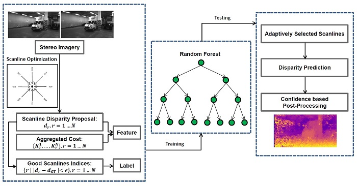
4.1.2. Random Forest Prediction

In addition, we analyze the quality of $r^{\ast }$ (see Section 3), which is the direct prediction of the random forest and the reference for further confidence based processing. Adaptive scanline selection based on a classification strategy is the core concept of SGM-Forest that is superior to the scanline average of the standard SGM. Hence, $r^{\ast }$ and the corresponding $d_p^{r^{\ast }}$ are necessary for further comparison between SGM-ForestS and SGM-ForestM.

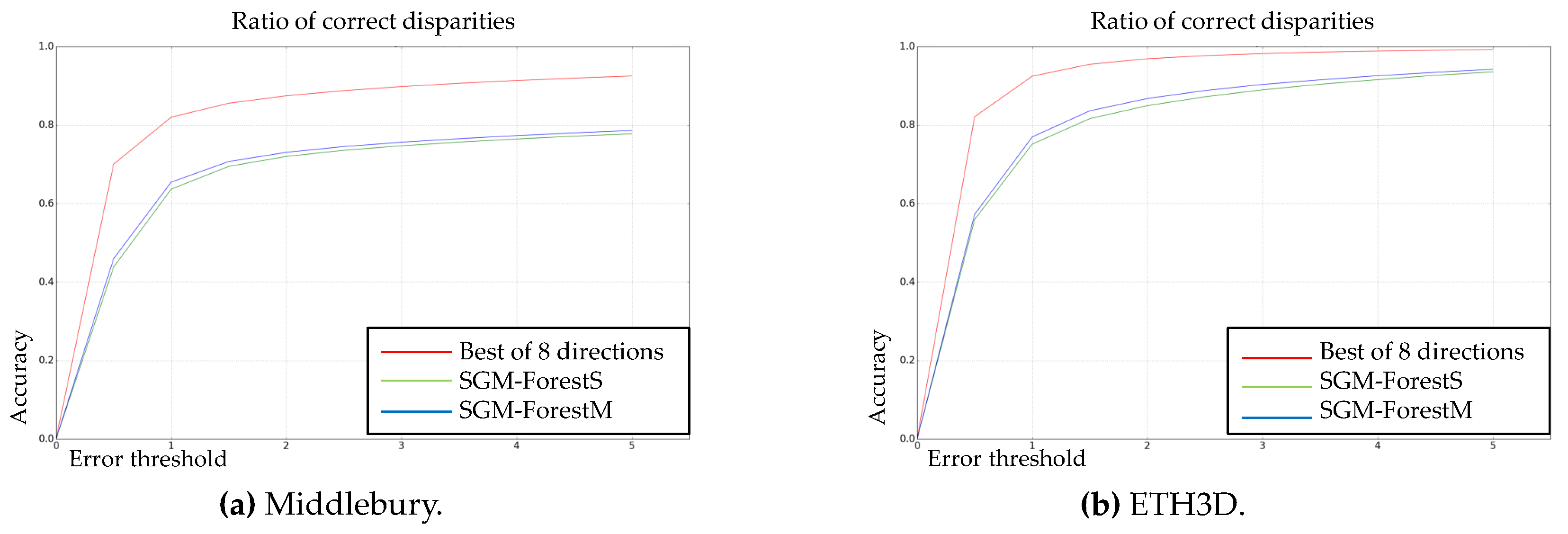
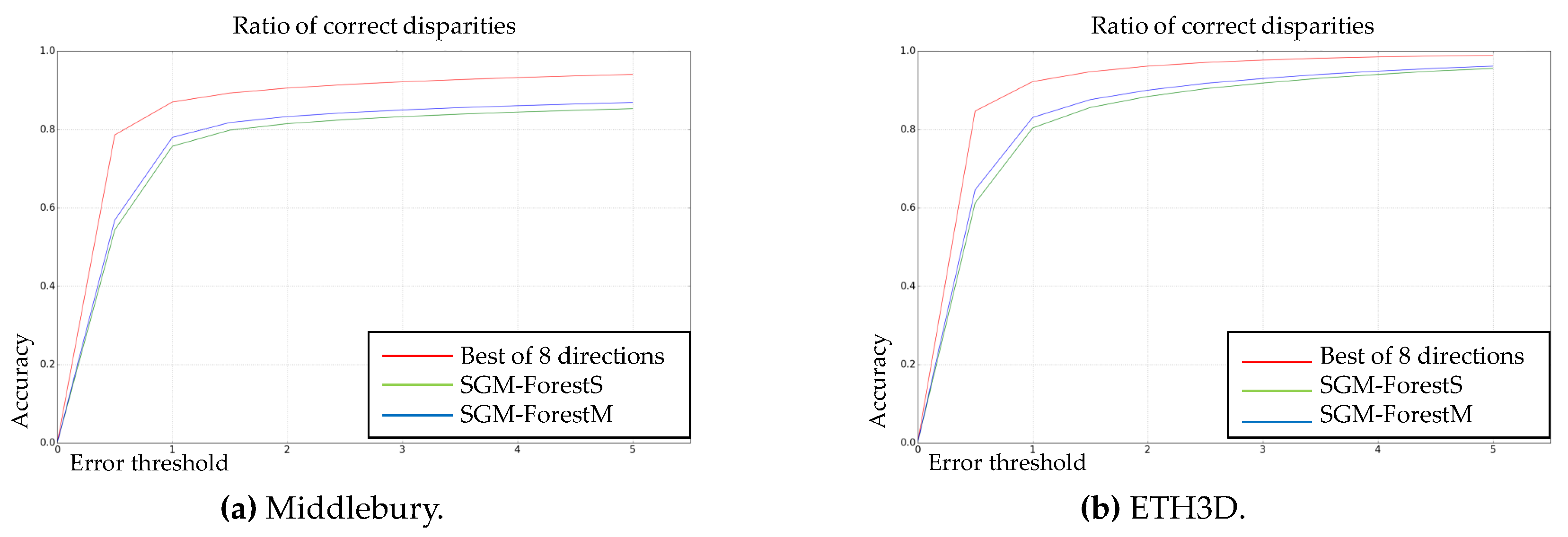
In Figure 3 and Figure 4, the error plots are displayed for SGM-ForestS, SGM-ForestM, and the upper bound of SO if the best scanline can always be selected from 8 alternatives. At here, it should be noted that the disparity prediction of the random forest ($d_p^{r^{\ast }}$) is directly compared to the ground truth for calculating the ratio of correct disparity estimation (y-axis), considering different estimation errors allowed (x-axis). We still test two matching cost algorithms (Census and MC-CNN-acrt) on two benchmark datasets (Middlebury and ETH3D).

The figures above show that both SGM-Forest implementations achieve good performance to approach the best SO, which demonstrates the feasibility of scanline selection based on a classification framework. In addition, SGM-ForestM is superior to SGM-ForestS in all cases. The results indicate that SGM-ForestM is essentially better at scanline prediction and capable of deriving preferable initial disparity values for further processing.

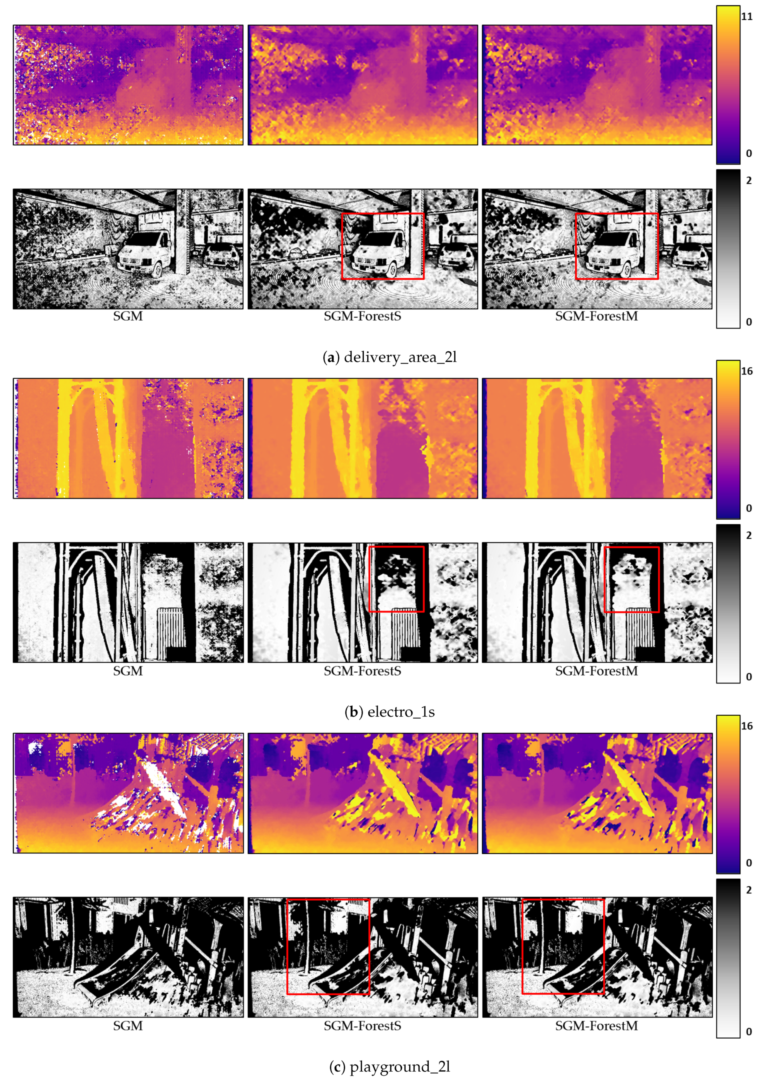
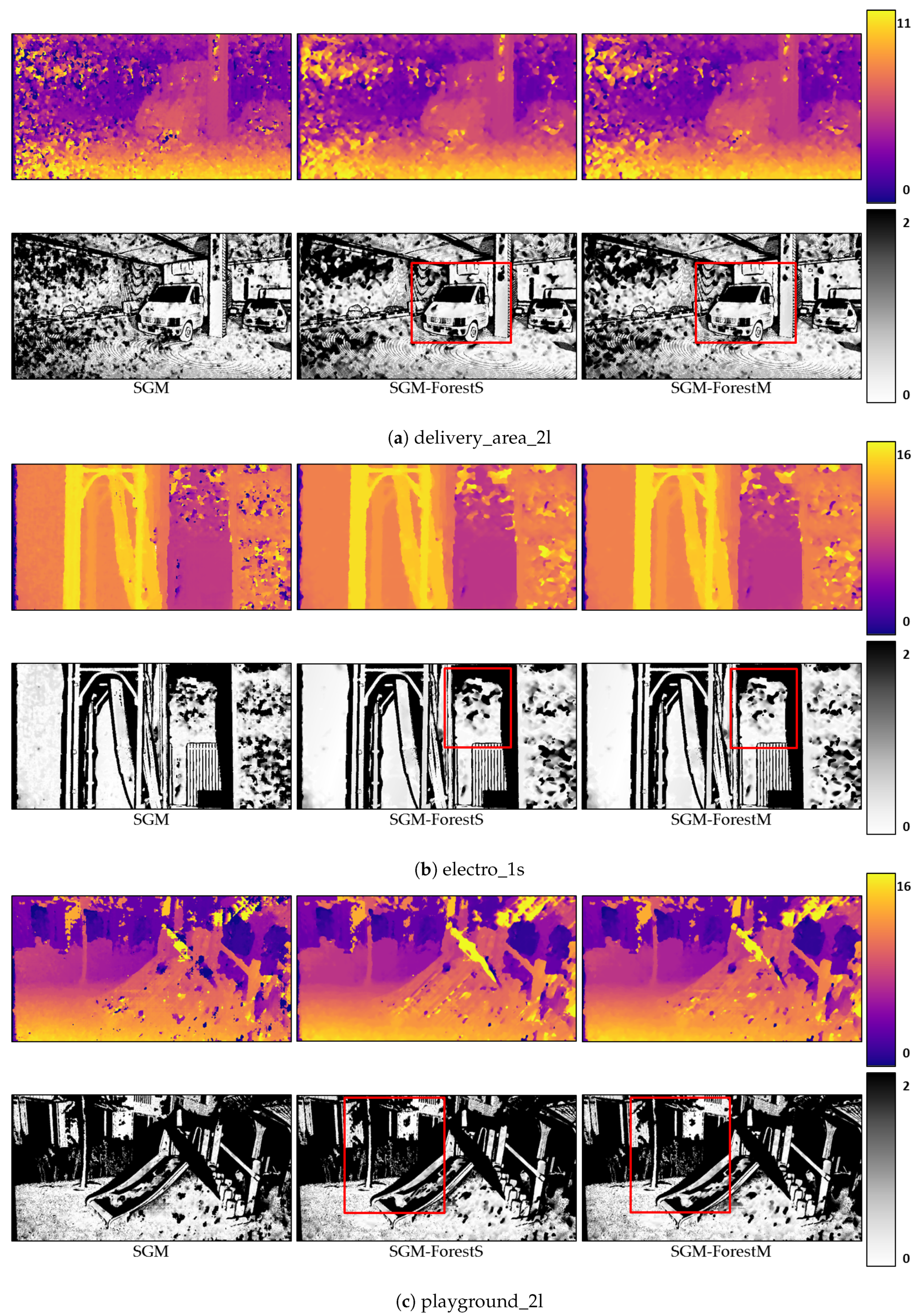
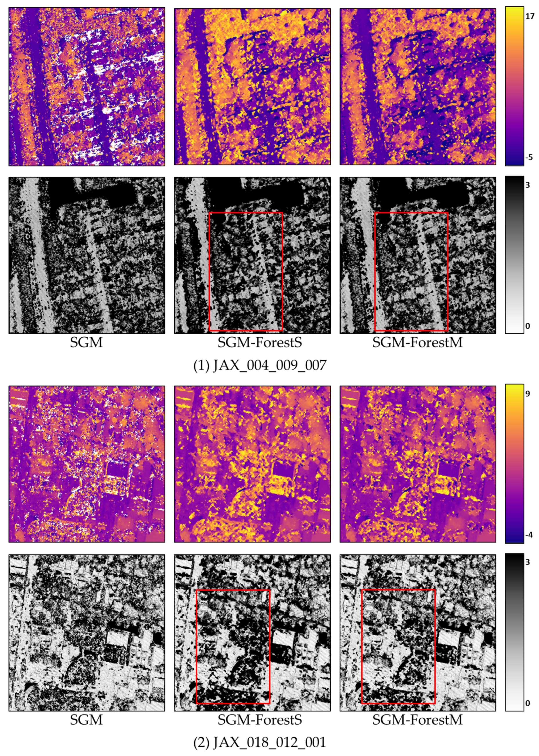
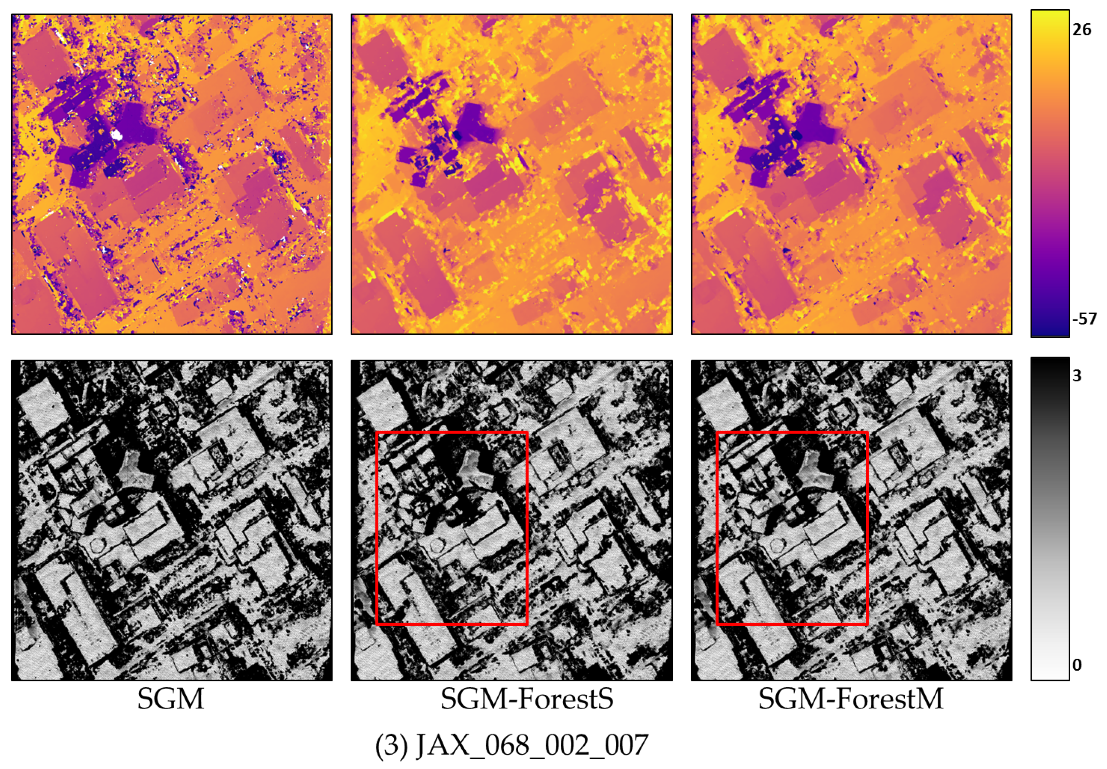
4.1.3. Qualitative Results

In this section, we select several stereo pairs from ETH3D to show the disparity maps generated based on SGM, SGM-ForestS, and SGM-ForestM, respectively. The corresponding error maps are displayed below. Regarding ‘2 pixel’ as the upper bound, all the pixels with an error above the bound are colored black, while the rest are colored uniformly according to the error as indicated by the color bar. We apply Census and MC-CNN-acrt to calculate the matching cost, respectively, and the results are displayed in Figure 5 and Figure 6.

In each subfigure, the disparity map and the error map for SGM, SGM-ForestS, and SGM-ForestM, respectively, are displayed from left to right, with a color bar at the end. The red rectangles marked in the error maps represent the main difference of the result between SGM-ForestS and SGM-ForestM. It is found that the disparity maps generated by the two SGM-Forest implementations are smoother than SGM. Moreover, according to the error map, SGM-ForestM suffers fewer errors compared with SGM-ForestS. Especially for the ill-posed regions (e.g., textureless areas, reflective surfaces, etc.), SGM-ForestM performs better as highlighted by the red rectangles.

4.2. Airborne and Satellite Datasets

Besides the close-range images, we also test the proposed algorithm on airborne data, the aerial image matching benchmark from EuroSDR, and on satellite data, from the pairwise semantic stereo challenge (Track 2) in the 2019 IEEE GRSS data fusion contest [18].

4.2.1. Airborne Dataset Experiment

The aerial image matching benchmark project is motivated by the development of matching algorithms and the improved quality of the elevation data obtained by advanced airborne cameras. Based on the benchmark datasets and the corresponding evaluation platform, the potential of the ongoing photogrammetric software is assessed by comparing their generated 3D products, including point clouds, digital surface models (DSM), and so forth.

The nadir airborne datasets, Vaihingen/Enz with moderate ground sampling distance (20 cm) and overlap (63% in flight and 62% cross flight), are used in this paper. We randomly select a stereo pair and apply SGM, SGM-ForestS, and SGM-ForestM to generate a disparity map, respectively. The master epipolar image and the corresponding result of each algorithm are displayed in Figure 7, with an area highlighted by a green rectangle to compare details.

According to the results above, it is still found that the two SGM-Forest implementations generate a smoother disparity map than the standard SGM. Within the highlighted region, SGM-ForestM suffers less noise than SGM-ForestS, which further demonstrates the superiority of the former.

4.2.2. Satellite Dataset Experiment

The 2019 IEEE GRSS data fusion contest provides the grss_dfc_2019 dataset [41], a subset of the Urban Semantic 3D (US3D) [17] data, including multi-view, multi-band satellite images and ground truth geometric and semantic labels. Several tasks are designed to reconstruct both a 3D geometric model and a segmentation of semantic classes for urban scenes, aiming at further supporting the research in stereo and semantic 3D reconstruction using machine intelligence and deep learning.

The contest data are captured by WorldView-3 satellite including RGB and 8-band visible and near infrared (VNIR) multi-spectral images, with ground sampling distance as approximately 35 cm. 26 images are collected between 2014 and 2016 over Jacksonville, Florida, and 43 images are collected between 2014 and 2015 over Omaha, Nebraska, United States. In our experiment, epipolar rectified stereo pairs from challenge track 2 are used, with pairwise ground truth disparity images generated using airborne LiDAR data. For evaluation, we only consider the reconstructed stereo geometry, ignoring the semantics information.

We apply SGM, SGM-ForestS, and SGM-ForestM, on 150 stereo pairs randomly selected from Jacksonville data. Due to the data inconsistency between the stereo images and LiDAR point clouds, the random forest is trained on ETH3D datasets for SGM-ForestS and SGM-ForestM. Thus, the robustness of the proposed algorithm is also tested when different data sources are used for training and validation.

When using 3 pixels as the upper limit of the allowed error, the validation accuracy for SGM, SGM-ForestS, and SGM-ForestM are 66.06%, 61.36%, and 67.18%, respectively. With different datasets to train the random forest, the performance of SGM-ForestS is limited and even surpassed by original SGM. The reason is the poor inference of the random forest when data different from the training sets are fed as input. However, SGM-ForestM is capable of providing more reliable scanline prediction, which is consistent with our demonstration in Figure 3 and Figure 4. Therefore, it performs the best. Some visualization results are displayed in Figure 8.

The reference LiDAR data were collected several years before the satellite images. Therefore, the images containing stable objects, for example, buildings, are selected for visualization and evaluation. It is found that SGM-ForestM is capable of better recovering the roads and buildings (as highlighted by the red rectangles).

5. Conclusions

In this paper, we propose SGM-ForestM as an extension of SGM-ForestS based on a multi-label classification strategy. Compared with the single scanline selection scheme of the latter using random forest, we collect all the promising scanlines, given that normally more than one scanline is capable of predicting the correct disparity. We test the method on several datasets from close-range imagery, to airborne and satellite data. The results indicate that SGM-ForestM performs better almost in all cases, since it reconstructs the ill-posed regions more reasonably, for example, textureless areas, reflective surfaces, and so forth. It is found that the inference of the random forest is improved when using the proposed multi-label scheme, leading to improvements between 0.5% to 2.3%, depending on the benchmark used.

In future work, the idea of adaptive scanline selection can be embedded to other stereo matching systems as a further optimization step, such as the Sgm-nets [23], or an end-to-end network. Furthermore, self-supervision is promising as the random forest has low demand on the number of training samples. A rigid standard can be set to exclude outliers for a reliable self-training.

References

1. Bleyer, M.; Breiteneder, C. Stereo matching—State-of-the-art and research challenges. In Advanced Topics in Computer Vision; Farinella, G.M., Battiato, S., Cipolla, R., Eds.; Springer: London, UK, 2013; pp. 143–179. [Google Scholar] [CrossRef]
2. Hirschmuller, H. Accurate and efficient stereo processing by semi-global matching and mutual information. In Proceedings of the 2005 IEEE Computer Society Conference on Computer Vision and Pattern Recognition (CVPR), San Diego, CA, USA, 20–25 June 2005; Volume 2, pp. 807–814. [Google Scholar] [CrossRef]
3. D’Angelo, P.; Reinartz, P. Semiglobal matching results on the ISPRS stereo matching benchmark. ISPRS—Int. Arch. Photogramm. Remote Sens. Spat. Inf. Sci. 2011, XXXVIII-4/W19, 79–84. [Google Scholar] [CrossRef] [Green Version]
4. D’Angelo, P. Improving semi-global matching: Cost aggregation and confidence measure. ISPRS—Int. Arch. Photogramm. Remote Sens. Spat. Inf. Sci. 2016, XLI-B1, 299–304. [Google Scholar] [CrossRef] [Green Version]
5. Hirschmüller, H. Stereo processing by semiglobal matching and mutual information. IEEE Trans. Pattern Anal. Mach. Intell. 2008, 30, 328–341. [Google Scholar] [CrossRef] [PubMed]
6. Scharstein, D.; Szeliski, R. A taxonomy and evaluation of dense two-frame stereo correspondence algorithms. Int. J. Comput. Vis. 2002, 47, 7–42. [Google Scholar] [CrossRef]
7. Hirschmüller, H. Semi-global matching-motivation, developments and applications. In Photogrammetric Week; Wichmann Verlag: Heidelberg, Germany, 2011; Volume 11, pp. 173–184. [Google Scholar]
8. Kuschk, G.; d’Angelo, P.; Qin, R.; Poli, D.; Reinartz, P.; Cremers, D. DSM accuracy evaluation for the ISPRS commission I image matching benchmark. ISPRS—Int. Arch. Photogramm. Remote Sens. Spat. Inf. Sci. 2014, XL-1, 195–200. [Google Scholar] [CrossRef] [Green Version]
9. Qin, R.; Huang, X.; Gruen, A.; Schmitt, G. Object-based 3-D building change detection on multitemporal stereo images. IEEE J. Sel. Top. Appl. Earth Observ. Remote Sens. 2015, 8, 2125–2137. [Google Scholar] [CrossRef]
10. Schönberger, J.L.; Sinha, S.N.; Pollefeys, M. Learning to fuse proposals from multiple scanline optimizations in semi-global matching. In Computer Vision—ECCV 2018; Ferrari, V., Hebert, M., Sminchisescu, C., Weiss, Y., Eds.; Springer International Publishing: Cham, Switzerland, 2018; pp. 758–775. [Google Scholar]
11. Menze, M.; Geiger, A. Object scene flow for autonomous vehicles. In Proceedings of the 2015 IEEE Conference on Computer Vision and Pattern Recognition (CVPR), Boston, MA, USA, 7–12 June 2015; pp. 3061–3070. [Google Scholar] [CrossRef] [Green Version]
12. Schöps, T.; Schönberger, J.L.; Galliani, S.; Sattler, T.; Schindler, K.; Pollefeys, M.; Geiger, A. A multi-view stereo benchmark with high-resolution images and multi-camera videos. In Proceedings of the 2017 IEEE Conference on Computer Vision and Pattern Recognition (CVPR), Honolulu, HI, USA, 21–26 July 2017; pp. 2538–2547. [Google Scholar] [CrossRef]
13. Scharstein, D.; Pal, C. Learning conditional random fields for stereo. In Proceedings of the 2007 IEEE Conference on Computer Vision and Pattern Recognition (CVPR), Minneapolis, MN, USA, 17–22 June 2007; pp. 1–8. [Google Scholar] [CrossRef]
14. Hirschmüller, H.; Scharstein, D. Evaluation of cost functions for stereo matching. In Proceedings of the 2007 IEEE Conference on Computer Vision and Pattern Recognition (CVPR), Minneapolis, MN, USA, 17–22 June 2007; pp. 1–8. [Google Scholar] [CrossRef]
15. Scharstein, D.; Hirschmüller, H.; Kitajima, Y.; Krathwohl, G.; Nešić, N.; Wang, X.; Westling, P. High-resolution stereo datasets with subpixel-accurate ground truth. In German Conference on Pattern Recognition (GCPR 2014); Springer: Münster, Germany, 2014; pp. 31–42. [Google Scholar]
16. Haala, N. Dense image matching final report. EuroSDR Publ. Ser. Off. Publ. 2014, 64, 115–145. [Google Scholar]
17. Bosch, M.; Foster, K.; Christie, G.A.; Wang, S.; Hager, G.D.; Brown, M.Z. Semantic Stereo for Incidental Satellite Images. In Proceedings of the 2019 IEEE Winter Conference on Applications of Computer Vision (WACV), Waikoloa Village, HI, USA, 7–11 January 2019; pp. 1524–1532. [Google Scholar]
18. Le Saux, B.; Yokoya, N.; Hansch, R.; Brown, M.; Hager, G.; Kim, H. 2019 IEEE GRSS Data Fusion Contest: Semantic 3D Reconstruction [Technical Committees]. IEEE Geosci. Remote Sens. Mag. 2019, 7, 103–105. [Google Scholar] [CrossRef]
19. Birchfield, S.; Tomasi, C. Depth discontinuities by pixel-to-pixel stereo. In Proceedings of the Sixth International Conference on Computer Vision (ICCV), Bombay, India, 4–7 January 1998; pp. 1073–1080. [Google Scholar] [CrossRef]
20. Ni, J.; Li, Q.; Liu, Y.; Zhou, Y. Second-Order Semi-Global Stereo Matching Algorithm Based on Slanted Plane Iterative Optimization. IEEE Access 2018, 6, 61735–61747. [Google Scholar] [CrossRef]
21. Zbontar, J.; LeCun, Y. Stereo matching by training a convolutional neural network to compare image patches. J. Mach. Learn. Res. 2016, 17, 1–32. [Google Scholar]
22. Luo, W.; Schwing, A.G.; Urtasun, R. Efficient Deep Learning for Stereo Matching. In Proceedings of the 2016 IEEE Conference on Computer Vision and Pattern Recognition (CVPR), Las Vegas, NV, USA, 27–30 June 2016; pp. 5695–5703. [Google Scholar] [CrossRef]
23. Seki, A.; Pollefeys, M. Sgm-nets: Semi-global matching with neural networks. In Proceedings of the 2017 IEEE Conference on Computer Vision and Pattern Recognition (CVPR), Honolulu, HI, USA, 21–26 July 2017; pp. 6640–6649. [Google Scholar] [CrossRef]
24. Scharstein, D.; Taniai, T.; Sinha, S.N. Semi-global stereo matching with surface orientation priors. In Proceedings of the 2017 International Conference on 3D Vision (3DV), Qingdao, China, 10–12 October 2017; pp. 215–224. [Google Scholar] [CrossRef] [Green Version]
25. Michael, M.; Salmen, J.; Stallkamp, J.; Schlipsing, M. Real-time stereo vision: Optimizing semi-global matching. In Proceedings of the 2013 IEEE Intelligent Vehicles Symposium (IV), Gold Coast, QLD, Australia, 23–26 June 2013; pp. 1197–1202. [Google Scholar] [CrossRef]
26. Poggi, M.; Mattoccia, S. Learning a general-purpose confidence measure based on O(1) features and a smarter aggregation strategy for semi global matching. In Proceedings of the 2016 Fourth International Conference on 3D Vision (3DV), Stanford, CA, USA, 25–28 October 2016; pp. 509–518. [Google Scholar] [CrossRef]
27. Zhang, F.; Prisacariu, V.; Yang, R.; Torr, P.H. GA-Net: Guided Aggregation Net for End-to-end Stereo Matching. In Proceedings of the IEEE Conference on Computer Vision and Pattern Recognition (CVPR), Long Beach, CA, USA, 15–21 June 2019; pp. 185–194. [Google Scholar]
28. Bromley, J.; Bentz, J.; Bottou, L.; Guyon, I.; LeCun, Y.; Moore, C.; Sackinger, E.; Shah, R. Signature Verification using a “Siamese” Time Delay Neural Network. Int. ]. Pattern Recognit. Artif. Intell. 1993, 7. [Google Scholar] [CrossRef] [Green Version]
29. Zabih, R.; Woodfill, J. Non-parametric local transforms for computing visual correspondence. In Computer Vision—ECCV’94; Eklundh, J.O., Ed.; Springer: Berlin/Heidelberg, Germany, 1994; pp. 151–158. [Google Scholar]
30. Duda, R.O.; Hart, P.E.; Stork, D.G. Pattern Classification, 2th ed.; Wiley: New York, NY, USA, 2001. [Google Scholar]
31. Boutell, M.R.; Luo, J.; Shen, X.; Brown, C.M. Learning multi-label scene classification. Pattern Recognit. 2004, 37, 1757–1771. [Google Scholar] [CrossRef] [Green Version]
32. McCallum, A. Multi-label text classification with a mixture model trained by EM. AAAI Workshop Text Learn. 1999, 1–7. [Google Scholar]
33. Schapire, R.E.; Singer, Y. BoosTexter: A boosting-based system for text categorization. Mach. Learn. 2000, 39, 135–168. [Google Scholar] [CrossRef] [Green Version]
34. Clare, A.; King, R.D. Knowledge discovery in multi-label phenotype data. In Principles of Data Mining and Knowledge Discovery; De Raedt, L., Siebes, A., Eds.; Springer: Berlin/Heidelberg, Germany, 2001; pp. 42–53. [Google Scholar]
35. Tsoumakas, G.; Katakis, I. Multi-label classification: An overview. Int. J. Data Warehous. Min. (IJDWM) 2007, 3, 1–13. [Google Scholar] [CrossRef] [Green Version]
36. Schumacher, F.; Greiner, T. Matching cost computation algorithm and high speed FPGA architecture for high quality real-time semi global matching stereo vision for road scenes. In Proceedings of the 17th International IEEE Conference on Intelligent Transportation Systems (ITSC), Qingdao, China, 8–11 October 2014; pp. 3064–3069. [Google Scholar] [CrossRef]
37. Gehrig, S.K.; Rabe, C. Real-time semi-global matching on the CPU. In Proceedings of the 2010 IEEE Computer Society Conference on Computer Vision and Pattern Recognition—Workshops, San Francisco, CA, USA, 13–18 June 2010; pp. 85–92. [Google Scholar] [CrossRef]
38. Arndt, O.J.; Becker, D.; Banz, C.; Blume, H. Parallel implementation of real-time semi-global matching on embedded multi-core architectures. In Proceedings of the 2013 International Conference on Embedded Computer Systems: Architectures, Modeling, and Simulation (SAMOS), Agios Konstantinos, Greece, 15–18 July 2013; pp. 56–63. [Google Scholar] [CrossRef]
39. Gehrig, S.K.; Eberli, F.; Meyer, T. A real-time low-power stereo vision engine using semi-global matching. In Computer Vision Systems; Fritz, M., Schiele, B., Piater, J.H., Eds.; Springer: Berlin/Heidelberg, Germany, 2009; pp. 134–143. [Google Scholar]
40. Banz, C.; Hesselbarth, S.; Flatt, H.; Blume, H.; Pirsch, P. Real-time stereo vision system using semi-global matching disparity estimation: Architecture and FPGA-implementation. In Proceedings of the 2010 International Conference on Embedded Computer Systems: Architectures, Modeling and Simulation, Samos, Greece, 19–22 July 2010; pp. 93–101. [Google Scholar] [CrossRef]
41. 2019 IEEE GRSS Data Fusion Contest. Available online: http://www.grss-ieee.org/community/technical-committees/data-fusion. (accessed on 26 November 2019).
Figure 1. The experimental image: the target pixels are marked in green.
Remotesensing 12 01069 g001
Figure 2. Stereo pair, cost cube and the corresponding aggregated cost cube in Semi-Global Matching (SGM).
Remotesensing 12 01069 g002
Figure 3. Error plots for SGM-ForestS, SGM-ForestM, and the upper bound of SO (Matching Cost: Census).
Remotesensing 12 01069 g003
Figure 4. Error plots for SGM-ForestS, SGM-ForestM, and the upper bound of SO (Matching Cost: MC-CNN-acrt).
Remotesensing 12 01069 g004
Figure 5. The disparity maps and the corresponding error maps. From left to right, the results of SGM, SGM-ForestS, and SGM-ForestM are displayed, respectively (Matching cost: Census).
Remotesensing 12 01069 g005
Figure 6. The disparity maps and the corresponding error maps. From left to right, the results of SGM, SGM-ForestS, and SGM-ForestM are displayed, respectively (Matching cost: MC-CNN-acrt).
Remotesensing 12 01069 g006
Figure 7. Stereo matching results on EuroSDR benchmark datasets (Vaihingen/Enz).
Remotesensing 12 01069 g007
Figure 8. Results on stereo datasets from the 2019 IEEE GRSS data fusion contest (Track 2, pairwise semantic stereo challenge).
Remotesensing 12 01069 g008aRemotesensing 12 01069 g008b