Article

An Optimal Population Modeling Approach Using Geographically Weighted Regression Based on High-Resolution Remote Sensing Data: A Case Study in Dhaka City, Bangladesh

1
Department of Geography and Environment, Jahangirnagar University, Savar, Dhaka-1342, Bangladesh
2
Faculty of Geo-information Science and Earth Observation, University of Twente, 7500 Enschede, The Netherlands
3
Department of Land Surveying and Geo-Informatics, The Hong Kong Polytechnic University, Hong Kong, China
4
International Initiative on Spatial Lifecourse Epidemiology (ISLE), 7500 Enschede, The Netherlands
*
Author to whom correspondence should be addressed.
Remote Sens. 2020, 12(7), 1184; https://doi.org/10.3390/rs12071184
Submission received: 23 January 2020 / Revised: 31 March 2020 / Accepted: 31 March 2020 / Published: 7 April 2020

Abstract

:
Traditional choropleth maps, created on the basis of administrative units, often fail to accurately represent population distribution due to the high spatial heterogeneity and the temporal dynamics of the population within the units. Furthermore, updating the data of spatial population statistics is time-consuming and costly, which underlies the relative lack of high-resolution and high-quality population data for implementing or validating population modeling work, in particular in low- and middle-income countries (LMIC). Dasymetric modeling has become an important technique to produce high-resolution gridded population surfaces. In this study, carried out in Dhaka City, Bangladesh, dasymetric mapping was implemented with the assistance of a combination of an object-based image analysis method (for generating ancillary data) and Geographically Weighted Regression (for improving the accuracy of the dasymetric modeling on the basis of building use). Buildings were extracted from WorldView 2 imagery as ancillary data, and a building-based GWR model was selected as the final model to disaggregate population counts from administrative units onto 5 m raster cells. The overall accuracy of the image classification was 77.75%, but the root mean square error (RMSE) of the building-based GWR model for the population disaggregation was significantly less compared to the RMSE values of GWR based land use, Ordinary Least Square based land use and building modeling. Our model has potential to be adapted to other LMIC countries, where high-quality ground-truth population data are lacking. With increasingly available satellite data, the approach developed in this study can facilitate high-resolution population modeling in a complex urban setting, and hence improve the demographic, social, environmental and health research in LMICs.

1. Introduction

An accurate spatial representation of population counts is important for e.g., risk assessment, policy-making, disaster management, accessibility modeling, poverty mapping, and adaptive strategies for human health [1,2,3,4]. Mapping the population distribution at a high-resolution became popular for producing high-resolution gridded population surfaces (HGPS), which have large benefits for many [5]. Traditionally, the census has been the main data source for such mapping. Yet, the census is normally conducted every 10 years, which is insufficient to fully capture the fast dynamics of the population changes over time. Using traditional methods to update population data frequently is time-consuming, costly, and even infeasible at a large scale [6].
Over the past decade, researchers have developed a wide range of methods for mapping the spatial distribution of the population with the aid of Geographic Information Systems (GIS) technology, which is used to create choropleth maps. As the population is not uniformly distributed over space within the administrative units [7], GIS-based discrete and aggregated choropleth maps cannot represent the spatial distribution of the population accurately [8]. Recently, several projects incorporated remote sensing (RS) derived datasets to model population distribution, such as Gridded Population of the World (GPW) [9], Global Rural-Urban Mapping Project (GRUMP) [10], LandScan Global [11], and WorldPop (Asia, Africa, and South America) [12]. Other studies that have been undertaken were based on the intrinsic features of RS imagery, such as image texture indices [13]. Those products, however, were mainly generated either at country [14] or at regional level [15], with spatial resolutions ranging from 100 m to 1 km. Unfortunately, this resolution cannot meet the demands in some specific areas or situations, such as emergency/disaster response and resource allocation. This is especially important in low- and middle-income countries (LMICs) where resources for conducting surveys are usually limited. Moreover, the accuracy of the population distribution products in urban areas and in the outskirts is lower due to the high heterogeneity of the urban features [16]. Given the increasing urbanization experienced worldwide, the demand for mapping and the understanding of population distribution at a high-resolution is increasing as well.
Dasymetric mapping is a particular cartographic representation of data, where census data are disaggregated into spatial units/grids with the aid of ancillary data to produce HGPS [17]. It can incorporate a variety of ancillary data, such as parcel and building information, into the mapping of the population distribution. As population density varies across different types of land use and even across different census units within the same type of land use, it is important to model the population distribution on the basis of fine-scale ancillary data, such as generating HGPSs at the building level. This is a challenging task, as building data (e.g., footprint, height) are not always available, although very-high-resolution (VHR) satellite images may provide a solution to do so. Previous works have used medium- to coarse-resolution RS images in population modeling [18,19,20,21]. Hence, opportunities for using the information on buildings derived from VHR satellite images in dasymetric mapping have not been fully explored yet. In addition, ordinary least square (OLS) regression has mainly been used for population distribution, under the assumption of a stable relationship between population density and a certain feature of a place, derived from ancillary data. This assumption is rarely true in the real world, as even in a small study area, many unobserved factors (e.g., percentage of land use, building use, and road density) may affect its stability. Geographically Weighted Regression (GWR) has been developed to overcome the assumption of stationarity.
The main goal of this study was to develop a population disaggregation model by incorporating information on buildings extracted from VHR satellite imagery and GWR into a dasymetric model. Our model was compared with a model that combines GWR with land use data, and with a model that combines OLS with both land use and building data.

2. Materials and Methods

2.1. Study Area

Dhaka, as the capital city of Bangladesh, has a history of more than 400 years [22]. It is located on the bank of the Buriganga river and surrounded by six rivers in total: the Balu and Sitalakhya rivers on the eastern side, the Turag and Buriganga rivers on the western side, the Tongi Khal on the northern side and the Dhaleshwari river to the south [23]. According to the 2011 National Census, the total urban area of Bangladesh equals 8867.42 km2, covering 6% of the total land of Bangladesh, and has a population of 35,094,684, which is 23.3% of the total population of the country. Dhaka has 6,970,105 inhabitants, with a population density of 55,169 people per km2, whereas the national population density equals 976 people per km2 [24]. There are 92 wards (the smallest administrative unit) in Dhaka City Corporation (DCC), which are divided across two parts of the city. One is Dhaka North City Corporation (DNCC) and the other is Dhaka South City Corporation (DSCC). Figure 1 shows the location of Dhaka City in the context of Asia.

2.2. Datasets

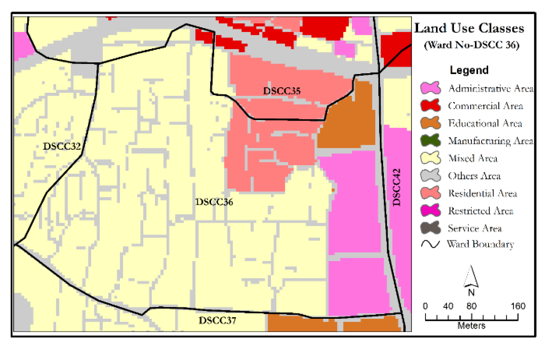
The population census is conducted every 10 years in Bangladesh, with the most recent one conducted in 2011. The tabular data of the population count against the smallest census unit (Ward in Bangladesh) were collected and the data are freely available on the website of the Bangladesh Bureau of Statistics (BBS). There are 92 wards in Dhaka City, divided across two parts—south and north. The land use data were collected from Rajdhani Unnayan Kartipakkha (RAJUK) and were produced in 2014. Furthermore, the data were categorized into eight types of inhabitable areas: administrative, commercial, educational, manufacturing, mixed, residential, restricted, and service areas. Remaining land areas were all categorized as non-inhabitable areas. The road network data in vector format (polygon) were also collected from RAJUK. The total road length of Dhaka is 1740 km, where Dhaka North has a road length of 1130 km and Dhaka South has a road length of 610 km. The minimum width of the road is 2.5 m and the maximum is 45 m. This road layer was used for the intersection process with the extracted buildings later, so that it moved the misclassified objects of the road to buildings. A recent multispectral WorldView 2 (WV2) image, acquired on 15 May 2017, at a high spatial resolution of 0.5 m, was obtained from DigitalGlobe and used for extracting buildings from the study area. WV2 has one panchromatic (450–800 nm) band with a resolution of 0.5 m, and eight multi-spectral bands (blue, coastal blue, green, yellow, red, red edge, NIR, NIR2) with a spatial resolution of 2 m for enhanced multispectral analyses. Together they are designed to improve the classification of land and aquatic features beyond any other space-based remote sensing platform.

2.3. Methods

The proposed method is a combination of Object based Image Analysis (OBIA) on VHR images, and GWR of the population distribution in the study area. Here, the extracted buildings of VHR were categorized according to land use. The areas of the buildings were used to calculate the proportion of building use, which were used in dasymetric methods later on. A framework of the proposed study is shown below (Figure 2).

2.3.1. Satellite Image Pre-Processing

The WorldView image was ortho-rectified and radiometrically corrected by the DigitalGlobe. The image included one single panchromatic band with a spatial resolution of 0.5 m and eight multi-spectral bands with a resolution of 2 m. A high pass filter (HPF) method was used for pan sharpening the multi-spectral bands [25].

2.3.2. OBIA for Building Extraction

OBIA is an interactive image analysis method, successfully used to extract information from VHR imagery [26]. It starts with the segmentation of imagery into homogeneous, meaningful objects. These objects are then further assigned to the classes of interest through classification. One of the main advantages of OBIA consists of its ability to incorporate not only spectral, but also textural and spatial information during the classification process. In this way, it can contribute to distinguishing objects that have the same spectral reflectance (e.g., buildings, roads, etc.). Considering these advantages, a segmentation process and a set of rules were defined in this study to extract the roofs of buildings. The entire building extraction process was performed in Trimble eCognition software. A multi-resolution segmentation [27] algorithm was used to segment WorldView 2 images into homogeneous objects. This algorithm relies on the following user-defined parameters: scale, shape and compactness. The shape parameter was set to 0.2 and the compactness parameter was set to 0.8. Different scale parameters were tried for segmentation, including 10, 20, 30, 40, and 50. In the end, a scale parameter of 30 was selected through visual interpretation of the segmentation results.
In our study area, the buildings vary in size and have different textural characteristics, due to the different construction materials. To address this challenge, a hierarchical classification process was designed and implemented. First, we classified the image into vegetation and non-vegetation classes. Second, we classified the non-vegetation class further into water, buildings and others classes (the remaining unclassified area). Various indices were used to define the classification rulesets, including the Normalized Difference Vegetation Index (NDVI), the Normalized Difference Water Index (NDWI) [28], the Green Band Ration (RatioG), image brightness value or mean spectral reflectance value of the green spectral band (Mean B3). Besides these indices, we also used spatial information, such as proximity, i.e., closeness to previously classified buildings. The threshold values for all input variables were set based on the trial and error method. Once the buildings were extracted from the image, they were further classified into eight building types, using the land use classes mentioned in Section 2.2.

2.3.3. Population Modeling

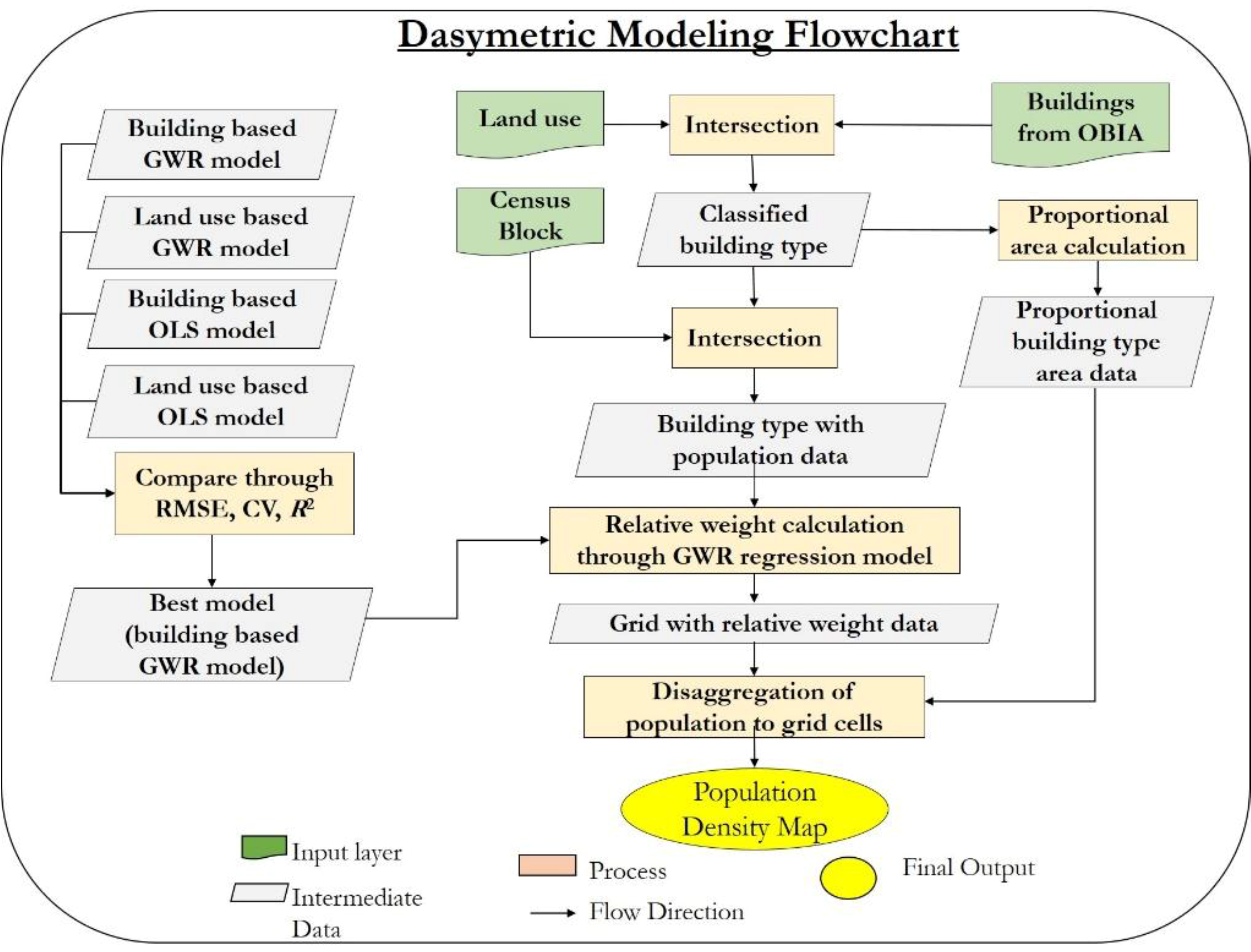
A modified dasymetric model was proposed to disaggregate the ward-level population onto 5x5 m grid cells. Initially, a GWR model was constructed to explore the relationship between the population density and each building type in each ward (i.e., variable population density for each building type across wards). GWR addresses the exact spatial regression as spatial non-stationarity and develops a relationship over space, which could be measured and mapped [29,30]. A generic regression equation [31], also applied to OLS-based models described in Equation (1), was used to illustrate this process:
p i = β 0 + j = 1 n ( β j   A i j ) + ε i
where pi is the census population of a ward i; βj is the population density for the building type j (or land use type j for OLS-based models); Aij is the area of the building type j (or land use type j for OLS-based models) within ward i; β0 and εi are the intercept and residual of the regression, respectively.
In each ward, the population density of each building type was multiplied by the area of each building, to calculate the absolute weight of each building. The absolute weight of each building was transformed into a relative weight by dividing it by the sum of the absolute weights of all buildings in the ward. The population of each ward was distributed onto each building based on relative weights. Finally, an areal weighting interpolator (AWI) method [32] was used to transform the population within buildings into the population within 5x5 m grid cells. Implementation started with intersecting grid cells and buildings. Some buildings were located entirely within one grid cell, but some were divided into two or more intersected zones by grid cell boundaries. The AWI method assumes that the population is uniformly distributed within a building. Thus, the population in each divided building was apportioned to each intersected zone on the basis of the areal proportion of that intersected zone over the building. The estimated population in all intersected zones and buildings completely located within each grid cell was then added to yield the total population in that grid cell. A detailed flowchart of dasymetric modeling is given in Figure 3. Spatial analyses were conducted in ArcGIS (version 10.5, ESRI).

2.3.4. Accuracy Assessment

The accuracy assessment was undertaken in two phases: one during the image classification and the other one during the population modeling. The accuracy assessment of the extracted buildings was performed by comparing the classification results with the reference data, which were collected from the visual interpretation of the study’s high-resolution image, using a random sampling method. Congalton suggested to have 75 to 100 samples for each class if the image covers a large area or if the classified image has a large number of Land use land cover (LULC) categories, such as more than 12 classes [33]. Hashemian et al. (2004) found that the accuracy results were stable for the large study area if the sample size was approximately 70 for each class [
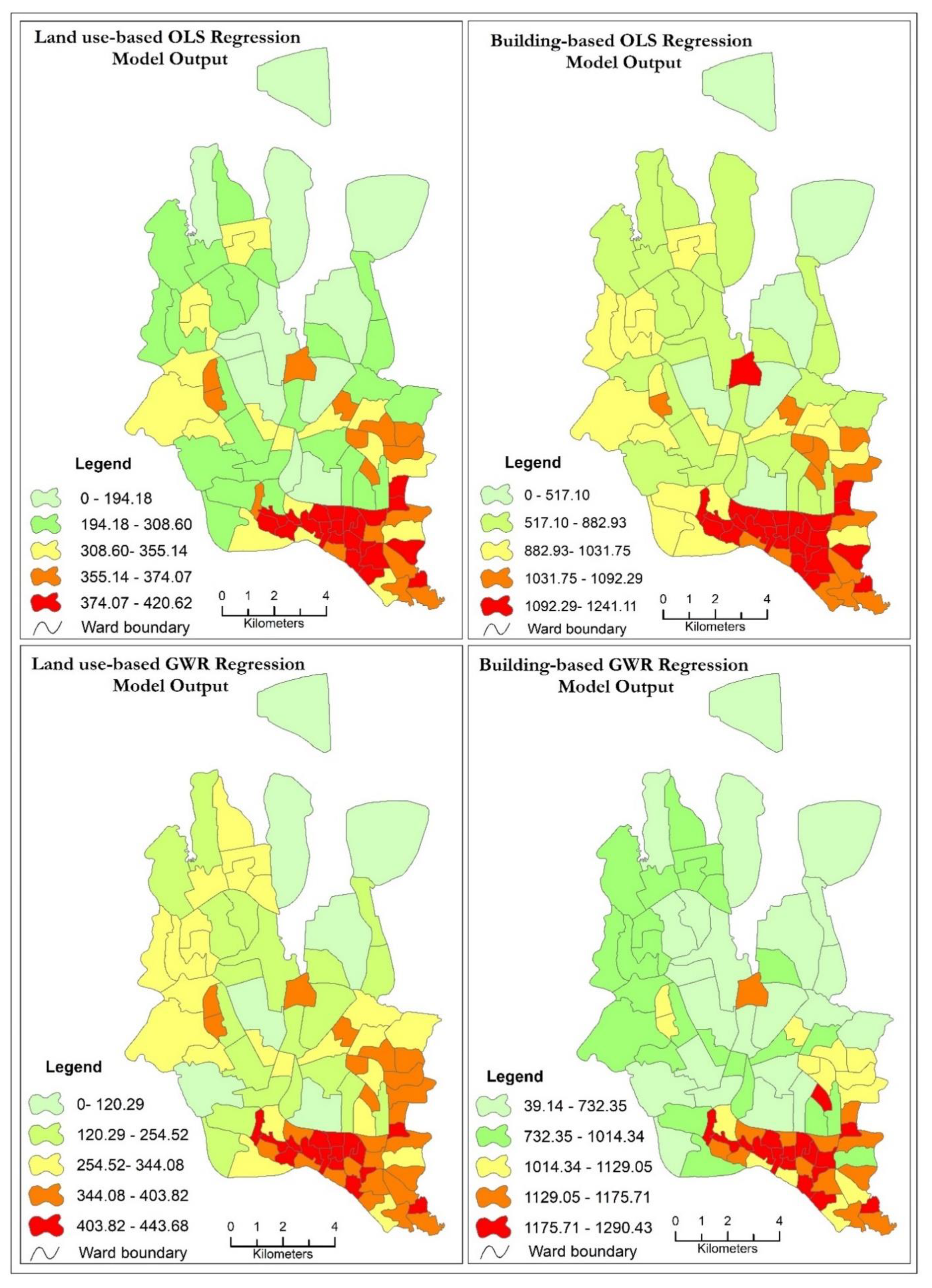
34]. However, this study area covers a very large area (136 sq. km) and the image was classified into four classes (i.e., buildings, water, vegetation, and others), so the reference sample size was fixed at 400 in total and 100 for each class. To assess the accuracy of the estimated population by the GWR model on the basis of building data, three regression models were constructed to estimate the population density over each building type or land use, including 1) using GWR based on land use data (i.e., variable density for each land use class across wards), 2) using OLS based on land use data (i.e., invariable density for each land use class across wards), and 3) using OLS based on building data (i.e., invariable density for each building type across wards). The root means square error (RMSE) and the coefficient of variance (CV) were calculated to compare the performance of the four models [5]:
RMSE = i = 1 n ( p i p ^ i ) 2 n
where, Pi is the population within ward i; p ^ i is the estimated population within ward i; and n is the number of wards. The CV was computed by dividing RMSE by the average building population within that ward.
To compare the variability among the different population models, we used another method: the coefficient of variance (CV). The CV is computed by dividing the RMSE with the average areal unit. In this research, the CV is calculated by dividing the RMSE by the ward-specific average population within that specific ward. This CV was calculated for each model by using the following equation (Equation (3)).
CV = R M S E p i ¯

3. Results

3.1. Accuracy Assessment of Buildings Extracted from WorldView2 Image

The multi-resolution segmentation process starts with an iterative process of local optimization based on the homogeneity of the created segments. The spectral homogeneity called “shape” is defined by the spectral reflectance of the pixels within the segment, and the value was set on 0.2 for this study area. Spatial homogeneity is based on two attributes—scale and compactness; 30 was fixed for scale and 0.8 was set for compactness by the visual interpretation of the segmentation results. Figure 4 shows the effects of shape, scale and compactness in the study area.
We obtained an overall accuracy of 77.75% and a kappa coefficient of 0.76. This is an acceptable accuracy given the complexity of the study area [35].
The classification results are shown in Table 1. The error matrix shows that the vegetation yielded the highest accuracy value in terms of both the producer’s and user’s accuracy; 100% and 96%, respectively. The next highest accuracy was water, with 92.98%, though the user’s accuracy shows a very poor value of 53%. The producer’s accuracy achieved for buildings was 73.91% and the user’s accuracy was 85%.
The main target for this OBIA was the identification of buildings’ roofs, whereas the remaining classes were categorized as the class “others”. The producer’s accuracy and user’s accuracy for the buildings class were 73.91% and 85%, respectively, which indicates the complexity of the study area.

3.2. Accuracy Asseessment of Models

A comparison of the GWR (based on building data) with the other three models (mentioned in Section 2.3.4) were carried out through RMSE and CV (Table 2). Here, the RMSE value is presented as the population count in the context of the total population of the study area. The total population of the study area was 6,970,105, and the average population count for each ward was 75,762. A comparison between the ward specific average population count and the RMSE of each model is shown in Figure 5. In addition, the output of each model is shown on the map, where it is clearly visible that the population density varies from model to model (Figure 6). The RMSE of model 1 shows a better value than model 2. Furthermore, the RMSE of model 3 is better than that of model 4. That means that the RMSE of the GWR model for both buildings-based and land use-based are better than the OLS regression models. However, among all four models, the GWR model based on building data shows the best result considering RMSE, Mean CV and adjusted R2.

3.3. Result of Population Disaggregation

The outputs of the dasymetric mapping of the study area at a 5 × 5 m spatial resolution are depicted in Figure 7. For comparison purposes, Figure 8 shows the output of the choropleth map of Dhaka city, which was produced using the total population divided by total ward area. The results of both maps show the significant difference in population distribution into grids. For example, Dhaka South City ward number 36 (DSCC36) has an area of 0.22 sq. km. The traditional choropleth map shows a population density of 2.95 people per 25 sq. m cell, considering the whole area of the census unit. Whereas only 0.074 sq. km is found as building area with five building types (administrative, commercial, educational, mixed and residential) (Figure 9). The dasymetric mapping shows five different population densities considering the different building types, such as administrative with 8.99, commercial with 9.33, educational with 9.08, mixed with 8.85, and residential with 9.24 person per 25 sq. m (Figure 10). Moreover, 66.80% of the land area of that census unit is used as the category “other land use”, where people do not live. This distribution gives a better understanding of the spatial distribution of the population than choropleth mapping.
The comparison between the predicted aggregated population and the ward size showed a very minimal difference from the actual population count in the dasymetric output (Figure 11). The minimum difference that was found in the population was 0 for 8 wards, 0 to 10 for 27 wards, 11 to 50 for 15 wards, 51 to 100 for 13 wards, 101 to 500 for 25 wards, 501 to 1000 for 3 wards, and a difference of 1054 was found in only 1 ward. Moreover, no pattern was found in the difference in the ward size of the studied city.

4. Discussion

4.1. OBIA-Based Classification Results

OBIA performed well at detecting the vegetation class. However, it obtained less satisfactory classification results for other classes, such as water and buildings. The water class was confused with other urban features, such as buildings. The reason behind this confusion was the construction materials used for the roofs of buildings. For example, every building has a water tank on top of the roof, which sometimes overflows. In addition, the shadows casted on different buildings also caused confusion between water and buildings.
The producer’s accuracy achieved for buildings was 73.91% and the user’s accuracy was 85%. The value of the producer’s accuracy metric is relatively low due to several reasons. First, the spectral reflectance of the roofs of buildings is similar to those of roads. Second, Dhaka city has a practice of roof gardening which increased the challenge of the buildings’ roof identification, leading to misclassification of the buildings class as a vegetation area. Furthermore, the accuracy of building detection depends on the segmentation results. The segmentation parameters such as scale, shape, and compactness were defined through trial and error and applied over the entire study area at once. Given the complexity of the study areas, the buildings were either over- or under-segmented during the segmentation process (Figure 12). Third, the classification rulesets in OBIA worked very well with identifying buildings in some less complex urban areas, yet, it performed worse in very complex areas (e.g., city center), where segmentation errors such as over-and under-segmentation occurred. Furthermore, the geometrical shape of the building varies across the investigated urban area. The buildings do not have a regular shape and size due to unplanned urbanization over the last four hundred years. Finally, the trees beside the buildings challenge the proper detection of the building shape.

4.2. Dasymetric Mapping

Population density is highly correlated with building type [6]. In developing countries, the urban area has different combinations of building use, which has an effect on population distribution. In addition, sometimes, there is no clear boundary for residential areas or they are all in mixed land classes, as the city grows in an unplanned way (e.g., Dhaka city). Consequently, population density may vary between residential areas and other areas, such as mixed or commercial building types, as we found in this study.
This study would have had better results if the following issues had been considered. Firstly, the height of the buildings was not considered in this model. As a result, the population density seemed very high in some cases as it assumed a horizontal distribution of pixels. Secondly, the geometric accuracy was not perfect, affecting the calculation of the total building area and consequently that of the population density. Thirdly, in this study, a generalized land use was used, where small segments of land use were merged within a big segment of land use. This may cause an inaccuracy in the area distribution of building types and in the distribution of population within the ward. Fourthly, the GWR model was used to calculate the proportional population among the building types within the ward.
The temporal variation in population and LULC data might impact the reported results. The population census was conducted in 2011, and was published in 2015 by the government. The LULC data was produced by another governmental organization (SoB) in 2008, and the VHR images of the study area were captured in May 2017.
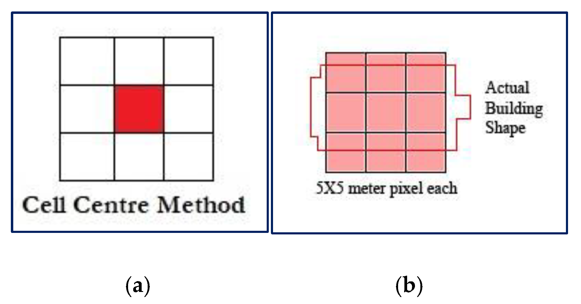
The conversion of the irregular vector shape file into a regular pixel may also impact the population disaggregation data. The cell center option (Figure 9) was selected as the cell assignment method during the pixel conversion. Cell assignment defines how the pixel will be assigned if more than one polygon falls within a pixel. Sometimes the 25 sq. m pixel did not fit the actual building shape, which affected the area calculation of the building. Figure 13 shows how the pixel conversion affects the area calculation of the actual building shape. The 5 m resolution may reduce this error, but not completely.

5. Conclusions

Studying population distribution in an appropriate and accurate way has become an important research area. The Geographic Information System, remote sensing, and geo-statistics are being used to support these population studies. Consequently, various techniques have been developed based upon resource availability, such as time, labor, data, and money and on fit to purpose as well. In this study, a dasymetric model containing the GWR model as well as building data, was developed to create a detailed dynamic population distribution model. This model was compared with three other different models incorporating GWR and OLS, based on building and land use data. The GWR demonstrated a high degree of probability of population density distribution using spatial non-stationarity from WorldView 2 imagery of Dhaka city. GWR appears to be an appropriate technique to improve the certainty of the population density distribution from images, taking the buildings’ characteristics of the urban environment into account. The developed model generated a gridded population distribution product with a resolution of 5 m for Dhaka city. In addition, the OBIA method was successfully used for building extraction from heterogeneous and complex urban areas. In the future, building height will be used in order to produce a more accurate population distribution.

Author Contributions

Conceptualization, P.J.; methodology, P.J.; software, P.J.; validation, P.J. and R.R.; formal analysis, R.R. and P.J.; investigation, P.J. and R.R.; resources, P.J. and R.R.; data curation, P.J. and R.R.; writing—original draft preparation, R.R. and P.J.; writing—review and editing, P.J. and R.R.; visualization, R.R. and P.J.; supervision, P.J.; project administration, P.J.; funding acquisition, P.J. All authors have read and agreed to the published version of the manuscript.

Funding

This research was partly funded by the State Key Laboratory of Urban and Regional Ecology of China, grant number SKLURE2018-2-5.

Acknowledgments

We thank the European Space Agency (ESA) for providing high-resolution satellite imagery, and Mariana Belgiu and Alfred Stein for their useful comments to improve the quality of this study.

Conflicts of Interest

The authors declare no conflict of interest. The funders had no role in the design of the study; in the collection, analyses, or interpretation of data; in the writing of the manuscript, or in the decision to publish the results.

References

  1. Jia, P.; Gaughan, A.E. Dasymetric modeling: A hybrid approach using land cover and tax parcel data for mapping population in Alachua County, Florida. Appl. Geogr. 2016, 66, 100–108. [Google Scholar] [CrossRef]
  2. Jia, P.; Shi, X.; Xierali, I.M. Teaming up census and patient data to delineate fine-scale hospital service areas and identify geographic disparities in hospital accessibility. Environ. monit. assess. 2019, 191, 303. [Google Scholar] [CrossRef] [PubMed] [Green Version]
  3. Maantay, J.; Maroko, A. Assessing population at risk: Areal interpolation and dasymetric mapping. In The Routledge Handbook of Environmental Justice, 1st ed.; Holifield, R., Chakraborty, J., Walker, G., Eds.; Routledge: New York, NY, USA, 2017; p. 670. [Google Scholar]
  4. Jia, P.; Anderson, J.D.; Leitner, M.; Rheingans, R. High-resolution spatial distribution and estimation of access to improved sanitation in Kenya. PLOS ONE 2016, 11, e0158490. [Google Scholar] [CrossRef] [PubMed] [Green Version]
  5. Jia, P.; Qiu, Y.; Gaughan, A.E. A fine-scale spatial population distribution on the high-resolution gridded population surface and application in Alachua County, Florida. Appl. Geogr. 2014, 50, 99–107. [Google Scholar] [CrossRef]
  6. Li, L.; Lu, D. Mapping population density distribution at multiple scales in Zhejiang Province using Landsat Thematic Mapper and census data. Int. J. Remote Sens. 2016, 37, 4243–4260. [Google Scholar] [CrossRef]
  7. Hay, S.I.; Noor, A.M.; Nelson, A.; Tatem, A.J. The accuracy of human population maps for public health application. Trop. Med. Int. Health 2005, 10, 1073–1086. [Google Scholar] [CrossRef] [PubMed]
  8. Martin, D. Directions in population GIS. Geogr. Compass 2011, 5, 655–665. [Google Scholar] [CrossRef]
  9. Balk, D.; Yetman, G. The Global Distribution of Population: Evaluating the Gains in Resolution Refinement. Center for International Earth Science Information Network (CIESIN), Columbia University. 2004. Available online: http://sedac.ciesin.columbia.edu/downloads/docs/gpw-v3/gpw3_documentation_final.pdf (accessed on 21 May 2017).
  10. CIESIN (Center for International Earth Science Information Network). Global Rural-Urban Mapping Project, Version 1 (GRUMPv1): Urban Extents Grid; Columbia University: New York, NY, USA, 2011. [Google Scholar] [CrossRef]
  11. Dobson, J.E.; Bright, E.A.; Coleman, P.R.; Durfee, R.C.; Worley, B.A. LandScan: A global population database for estimating populations at risk. Photogramm. Eng. Remote Sens. 2000, 66, 849–857. [Google Scholar] [CrossRef]
  12. Tatem, A.J.; Gaughan, A.E.; Stevens, F.R.; Patel, N.N.; Jia, P.; Pandey, A.; Linard, C. Quantifying the effects of using detailed spatial demographic data on health metrics: A systematic analysis for the AfriPop, AsiaPop, and AmeriPop projects. Lancet 2013, 381, S142. [Google Scholar] [CrossRef]
  13. Chen, K. An approach to linking remotely sensed data and areal census data. Int. J. Remote Sens. 2002, 23, 37–48. [Google Scholar] [CrossRef]
  14. Lu, D.; Weng, Q.; Li, G. Residential population estimation using a remote sensing derived impervious surface approach. Int. J. Remote Sens. 2006, 27, 3553–3570. [Google Scholar] [CrossRef]
  15. Sutton, P.C.; Taylor, M.J.; Elvidge, C.D. Using DMSP OLS imagery to characterize urban populations in developed and developing countries. In Remote Sensing of Urban and Suburban Areas; Rashed, T., Jürgens, C., Eds.; Springer: Dordrecht, The Netherlands; Berlin/Heidelberg, Germany, 2010; pp. 329–348. [Google Scholar] [CrossRef]
  16. Yang, X.; Ye, T.; Zhao, N.; Chen, Q.; Yue, W.; Qi JJ Zeng, B.; Jia, P. Population Mapping with Multisensor Remote Sensing Images and Point-Of-Interest Data. Remote Sens. 2019, 11, 574. [Google Scholar] [CrossRef] [Green Version]
  17. Mennis, J. Generating surface models of population using dasymetric mapping. Prof. Geogr. 2003, 55, 31–42. [Google Scholar] [CrossRef]
  18. Eicher, C.L.; Brewer, C.A. Dasymetric Mapping and Areal Interpolation: Implementation and Evaluation. Cartogr. Geogr. Inf. Sci. 2001, 28, 125–138. [Google Scholar] [CrossRef]
  19. Vijayaraj, V.; Bright, E.A.; Bhaduri, B.L. High resolution urban feature extraction for global population mapping using high performance computing. IEEE 2008, 1, 278–281. [Google Scholar]
  20. Tenerelli, P.; Gallego, J.F.; Ehrlich, D. Population density modelling in support of disaster risk assessment. Int. J. Disaster Risk Reduct. 2015, 13, 334–341. [Google Scholar] [CrossRef]
  21. Wei, C.; Taubenbock, H.; Blaschke, T. Measuring urban agglomeration using a city-scale dasymetric population map: A study in the Pearl River Delta, China. Habitat Int. 2017, 59, 32–43. [Google Scholar] [CrossRef] [Green Version]
  22. Ahmed, S.J.; Nahiduzzaman, K.M.; Bramley, G. From a town to a megacity: 400 years of growth. In Dhaka Megacity: Geospatial Perspectives on Urbanisation, Environment and Health; Dewan, A., Corner, R., Eds.; Springer: Dordrecht, The Netherlands; Berlin/Heidelberg, Germany; New York, NY, USA, 2014; p. 423. [Google Scholar]
  23. Zaman, A.M. Dhaka and Her Rivers: A Beautiful Relationship Gone Sour | 2017, August 7; The Daily Star. Available online: http://www.thedailystar.net/opinion/environment/dhaka-and-her-rivers-1444537 (accessed on 9 October 2017).
  24. Bangladesh Bureau of Statistis, (BBS). Population and Housing Census 2011: National Report, Volume-1, Analytical Report; Bangladesh Bureau of Statistics, Ministry of Planning: Dhaka, Bangladesh, 2011. [Google Scholar]
  25. Li, H.; Jing, L.; Tang, Y.; Liu, Q.; Ding, H.; Sun, Z.; Chen, Y. Assessment of pan-sharpening methods applied to WorldView-2 image fusion. In Proceedings of the International Geoscience and Remote Sensing Symposium (IGARSS), 2015-Novem, Milan, Italy, 26–31 July 2015; pp. 3302–3305. [Google Scholar] [CrossRef]
  26. Blaschke, T. Object based image analysis for remote sensing. ISPRS J. Photogramm. Remote Sens. 2010, 65, 2–16. [Google Scholar] [CrossRef] [Green Version]
  27. Baatz, M.; Schäpe, A. Multiresolution segmentation: An optimization approach for high quality multi-scale image segmentation. In Angewandte Geographische Informations—Verarbeitung XII; Strobl, J., Blaschke, T., Griesebner, G., Eds.; Wichmann: Karlsruhe, Germany, 2000; pp. 12–23. [Google Scholar]
  28. Gao, B.C. NDWI—A normalized difference water index for remote sensing of vegetation liquid water from space. Remote Sens. Environ. 1996, 58, 257–266. [Google Scholar] [CrossRef]
  29. Liu, X.; Herold, M. Population estimation and interpolation using remote sensing. In Urban Remote Sensing, 1st ed.; Weng, Q., Quattrochi, D.A., Eds.; CRC Press: Boca Raton, FL, USA, 2006; p. 450. [Google Scholar]
  30. Fotheringham, A.S.; Brunsdon, C.; Charlton, M.E. Geographically Weighted Regression: The Analysis of Spatially Varying Relationships; Wiley: Chichester, UK, 2002. [Google Scholar]
  31. Wu, C.; Murray, A.T. Population estimation using landsat enhanced thematic mapper imagery. Geogr. Anal. 2007, 39, 26–43. [Google Scholar] [CrossRef]
  32. Goodchild, M.F.; Lam, M.S. Areal Interpolation: A Variant of the Traditional Spatial Problem; Department of Geography, University of Western Ontario: London, UK, 1980; Volume 1, pp. 297–331. [Google Scholar]
  33. Congalton, R.G. A review of assessing the accuracy of classifications of remotely sensed data. Remote Sens. Environ. 1991, 37, 35–46. [Google Scholar] [CrossRef]
  34. Hashemian, M.S.; Abakar, A.A.; Fatemi, S.B. Study of sampling methods for accuracy assessment of classified remotely sensed data. In Proceedings of the 20th International Society for Photogrammetry and Remote Sensing Congress, Istanbul, Turkey, 12–23 July 2004; pp. 12–23. [Google Scholar]
  35. Foody, G. Harshness in image classification accuracy assessment. Int. J. Remote Sens. 2008, 29, 3137–3158. [Google Scholar] [CrossRef] [Green Version]
Figure 1. Location map of the study area in the context of various administrative units of Bangladesh and Asia.
Remotesensing 12 01184 g001
Figure 2. A framework of the research.
Remotesensing 12 01184 g002
Figure 3. A detailed flowchart of the disaggregation of the population based on building-based GWR.
Remotesensing 12 01184 g003
Figure 4. Segmented image (buildings) with scale 30, the shape and compactness parameters are 0.2 and 0.8, respectively.
Remotesensing 12 01184 g004
Figure 5. The figure shows the comparative analysis between the ward specific population count and the RMSE of each model, where the building based GWR model gives a better result than any other model. The result also gives an idea of how much the results differ from the actual average population.
Remotesensing 12 01184 g005
Figure 6. Population density distribution map of different models’ outputs. The class intervals were calculated following geometrical calculation, and the density was calculated in the areal unit of acres.
Remotesensing 12 01184 g006
Figure 7. Output of the 5 × 5 m raster-based dasymetric mapping of the study area.
Remotesensing 12 01184 g007
Figure 8. Output of the choropleth map of the study area.
Remotesensing 12 01184 g008
Figure 9. Raster-based land use map of sample ward Dhaka South 36 (DSCC36).
Remotesensing 12 01184 g009
Figure 10. 5 × 5 m raster-based Dasymetric mapping of sample ward Dhaka South 36 (DSCC36).
Remotesensing 12 01184 g010
Figure 11. The figure shows the pattern of the population count predicted from the dasymetric model against the ward size. No pattern is found between ward size and population count.
Remotesensing 12 01184 g011
Figure 12. Visualization of over- and under-segmented errors of buildings. (a) The red line corresponds to an over-segmentation result, whereas the whole white color represents the building. (b) The green line corresponds to an under-segmentation result, whereas some portions of the building (white color) merged with other urban features (purple color).
Remotesensing 12 01184 g012
Figure 13. Error in the pixel conversion process. (a) image shows the cell center conversion process and (b) image shows the error that occurred during the conversion.
Remotesensing 12 01184 g013
Table 1. Classification results obtained using Object Based Image Analysis (OBIA) technique.
Reference Data
Classification dataClass NameBuildingsOthersVegetationWaterTotalUser Accuracy (%)
Buildings85150010085
Others19770410077
Vegetation0496010096
Water113605310053
Total1151329657400
Producer Accuracy (%)73.9158.3310092.98Overall Accuracy 77.75 %
Kappa Coefficient 0.76
Table 2. Comparison of the accuracy of four different models based on RMSE, CV and adjusted R2.
Model NoModel NameRMSEMean CVAdjusted R2Rank
1GWR based on Building data191060.1830.721
2OLS based on Building data256760.2530.593
3GWR based on Land use data201600.1860.692
4OLS based on Land use data262590.2660.554

