Rapid Determination of Soil Class Based on Visible-Near Infrared, Mid-Infrared Spectroscopy and Data Fusion


1
Institute of Agricultural Remote Sensing and Information Technology Application, College of Environmental and Resource Sciences, Zhejiang University, Hangzhou 310058, China
2
INRAE, Unité InfoSol, 45075 Orléans, France
3
Institute of Digital Agriculture, Zhejiang Academy of Agricultural Sciences, Hangzhou 310021, China
4
Key Laboratory of Spectroscopy Sensing, Ministry of Agriculture, Hangzhou 310058, China
*
Author to whom correspondence should be addressed.
Remote Sens. 2020, 12(9), 1512; https://doi.org/10.3390/rs12091512
Submission received: 27 March 2020
/
Revised: 18 April 2020
/
Accepted: 20 April 2020
/
Published: 9 May 2020
(This article belongs to the Special Issue Estimation and Mapping of Soil Properties Based on Multi-Source Data Fusion)
Abstract
:Wise soil management requires detailed soil information, but conventional soil class mapping in a rather coarse spatial resolution cannot meet the demand for precision agriculture. With the advantages of non-destructiveness, rapid cost-efficiency, and labor savings, the spectroscopic technique has proved its high potential for success in soil classification. Previous studies mainly focused on predicting soil classes using a single sensor. In this study, we attempted to compare the predictive ability of visible near infrared (vis-NIR) spectra, mid-infrared (MIR) spectra, and their fused spectra for soil classification. A total of 146 soil profiles were collected from Zhejiang, China, and the soil properties and spectra were measured by their genetic horizons. Along with easy-to-measure auxiliary soil information (soil organic matter, soil texture, color and pH), four spectral data, including vis-NIR, MIR, their simple combination (vis-NIR-MIR), and outer product analysis (OPA) fused spectra, were used for soil classification using a multiple objectives mixed support vector machine model. The independent validation results showed that the classification model using MIR (accuracy of 64.5%) was slightly better than that using vis-NIR (accuracy of 64.2%). The predictive model built on vis-NIR-MIR did not improve the classification accuracy, having the lowest accuracy of 61.1%, which likely resulted from an over-fitting problem. The model based on OPA fused spectra performed best with an accuracy of 68.4%. Our results prove the potential of fusing vis-NIR and MIR using OPA for improving prediction ability for soil classification.
1. Introduction
It is well known that soils have high spatial heterogeneity with different intrinsic and morphological characteristics. Therefore, it is necessary to have a good understanding of soil on a local scale for better soil management. In practice, soil class is a good indicator for characterizing soil information and provides a basis for subsequent land management, land resource evaluation, crop planting, and fertilization [1].
Traditionally, soil classification depends on field surveys, laboratory analyses, and expert knowledge [2]. Conventional laboratory analyses are complex, time-consuming, expensive, and destructive [3,4,5]. Therefore, fast and non-destructive methods are needed for soil classification. Spectroscopic technology, with the advantages of being efficient, fast, convenient, and inexpensive, is widely applied in pedology [6,7,8,9].
Visible-near infrared (vis-NIR) spectroscopy has proved its ability in predicting many soil properties simultaneously [10,11,12], such as soil organic carbon, pH, cation exchanged capacity (CEC), clay content, total nitrogen, air-dry gravimetric water content, mineralogical content, and so on [13,14,15,16,17]. It is generally recognized that soil texture, soil organic matter (SOM), and iron and aluminum oxide could be predicted via vis-NIR spectra successfully [18,19,20]. Mid-infrared (MIR) spectroscopy is another commonly used technique for soil properties estimation with high accuracy [21,22]. MIR usually performs better than vis-NIR when predicting some properties, such as soil water content, texture, soil carbon, pH, and others [8,23] because vis-NIR spectra are dominated by weak overtones and combinations of fundamental vibrational bands for H–C, H–N, and O–H bonds that occur in the MIR region [4,6].
Despite great achievements in predicting soil classes and properties using soil spectroscopy, most previous studies focused on single domains and used either vis-NIR or MIR spectra. However, soil is a complex medium, so the use of either vis-NIR or MIR cannot cover enough soil information to analyze all of the soil properties [12]. Due to the heterogeneity of soil, the models based on single sensors are less stable [24]. An effective way to overcome the above weaknesses is data fusion, which integrates data from multiple sensors. Recently, some studies predicted soil properties by integrating different sensors [25,26,27,28]. Previous studies proved the potential of improving model performance using data fusion from multiple sensors [29,30,31]. For some soil attributes that were not previously predicted well by a single sensor, better prediction results can be obtained after data fusion [32,33]. Consequently, data fusion gives us a new way to classify different soils.
As for studies on soil classification using spectra, two approaches are mainly used. The first approach is to classify soil classes by characteristics of the soil spectral curves [20,34,35,36,37,38,39]. The second approach is based on the relationship between soil spectra and existing soil classification references. Many early studies on soil classification using spectra were carried out only on topsoil or on a certain horizon from the soil profile [40,41,42]. For these studies focusing on topsoil, they presented a classification accuracy between 44.4% and 96% [40,41,42,43]. However, this is not the best strategy since most soil classification systems are based on multiple horizons [2,20], which prompted several studies to move from a single soil layer to an entire soil profile [20,44]. To contain all soil horizons of the soil profile, a support vector machine (SVM) combined with the majority-voting method was proposed [45]. Currently, soil properties and environmental covariates are considered the main parameters to classify soils. When considering the properties and environmental data, the prediction results of soil types have achieved high accuracy as well [43,46]. As for the studies considering multiple horizons and environmental factors, they presented a classification accuracy between 57% and 83% [2,44,45,46]. Although the accuracies are not better than those focusing on topsoil, the factors considered in the study are more comprehensive.
The aim of this study is as follows: (1) to compare the ability of vis-NIR and MIR spectral to classify soils, (2) to compare the prediction capability of different methods of data fusion, such as simple combination and OPA, and (3) to compare the prediction capability of data from single sensors with data from multiple sensors.
2. Materials and Methods
2.1. Study Area and Soil Sampling Sites
This study was carried out in Zhejiang Province, China, with latitudes ranging from 27–31.5°N and longitudes from 118–123°E. The study covers an area of more than 105,000 km2 with the elevation ranging from 0 to 1907 m. The annual rainfall and annual average temperature are approximately 1100 to 1900 mm and 16.5 °C, respectively. In this study area, the most widely distributed soil types are Anthrosols and Cambosols, covering more than 55% of the total land mass. On alluvial plains and the highlands, Primosols are widely distributed. Argosols and Ferrosols mainly occur in the highlands. In addition, the sum of Halosols, Gleyosols and Isohumosols only represents less than 4% of the study area.
A total of 146 soil profiles were collected from Zhejiang Province between 2009 and 2012, resulting in 571 soil samples from each genetic horizon of these soil profiles. All soil samples were air-dried, ground and sieved to less than 2 mm. The samples were then sent to the laboratory for measurement of the physical and chemical properties as well as the spectral data (vis-NIR and MIR). The sample positions are shown in Figure 1. The soil classification for each soil profile was determined by an experienced soil judge based on the Chinese Soil Taxonomy (CST) [47].
2.2. Chemical Analysis
In this study, we selected soil organic matter, texture, moist color and pH as auxiliary soil information to build the classification model. Organic matter was measured through the H2SO4-K2Cr2O7 oxidation method. Texture was measured through a pipette method. Soil pH was measured in 1:1 soil/water suspension, with the potentiometric method [49]. Soil moist color was recorded by a Munsell soil system [50]. In addition, the colors recorded by the Munsell color system were hard to apply to the classification algorithm. Thus, we transformed soil color data to RGB using the aqp package [51] in R 3.5.3. [52].
2.3. Spectroscopic Measurement and Pre-Processing
The vis-NIR spectral data was obtained with a FieldSpec® ProFR vis–NIR spectrometer (Analytical Spectral Devices, Boulder, CO, USA). The spectral range of the instrument is from 350 to 2500 nm. The instrument has a spectral resolution of 3 nm between 350 and 1000 nm and a spectral resolution of 10 nm between 1000 and 2500 nm. The resampling resolution of the spectra is 1 nm. For each measurement, a Spectralon® panel with 99% reflectance was used as the standard to calibrate the spectrometer. For every soil sample, we measured the vis-NIR spectra at three random positions with 10 internal replicates. Afterwards, we averaged the total 30 spectral data as the final spectra for each soil sample.
The MIR spectral data was obtained using the Agilent 4300 Handheld FTIR (Fourier transform infra-red) (Agilent Technologies, Santa Clara, CA, USA). The spectral range of this instrument is from 4000 to 650 cm−1. We used a DTGS (deuterated triglycine sulphate) detector with a spectral resolution of 4 cm−1 to measure the soil MIR spectra. The measurement and preparation methods of soil samples were the same as those used for vis-NIR.
For the vis-NIR spectra, due to the high signal-to-noise ratio, the spectral regions of 350 to 399 nm and 2451 to 2500 nm were removed. Then, the vis-NIR and MIR spectra were resampled to 10 nm and 6 cm−1, respectively. After several comparisons of the spectral pre-processing methods, we adopted the Savitzky-Golay algorithm to smooth the spectra. A polynomial of order 2 and window size 11 were used, and continuum removal (CR) followed.
2.4. Outer Product Analysis (OPA)
Outer product analysis is a data fusion algorithm. By analyzing the variance of the intervariable data matrix, the OPA process can calculate the frequencies between these two spectral domains [53]. Therefore, OPA has the potential to emphasize the co-evolution of different spectral domains and to determine whether there is any hidden information between the vis-NIR spectra and the MIR spectra [54]. For instance, for n soil samples having vis-NIR and MIR spectra with x and y wavelengths, we could acquire the intensities of each domain to construct two data vectors. We can naturally infer that the data vectors from the vis-NIR domain are the x dimension, the data vectors from the MIR domain are the y dimension and the number of both kinds of data vectors is n. Subsequently, we multiply both intensities to construct n new data matrixes (x rows by y columns), which contain all possible products of the intensities from the two vectors. Then, this matrix will be unfolded to n (x × y) vectors, which can be applied to further statistical analysis. Moreover, these vectors can be concatenated to a product matrix, called the outer product matrix, with n rows and x × y columns. This method was implemented in R 3.5.3. Figure 2 shows a workflow of data fusion by OPA.
For OPA analysis, the spectra of MIR (549 variables) were multiplied by the spectra of vis-NIR (216 variables), which resulted in a matrix with 113094 variables (549 × 216) for each soil sample. To overcome data redundancy and improve the computing efficiency, we used principal component analysis (PCA) to reduce the dimension of the fused data.
2.5. Model Construction
To ensure that all representative soil profiles can be completely covered in the calibration set, data partitioning was made at the soil suborder level. At the soil suborder level, a stratified random sampling method was used with a 2:1 ratio of calibration and validation samples. Nevertheless, few soil samples belonged to Orthic Anthrosol or Anthric Primosol. These soil profiles were allocated to the calibration dataset and none were allocated to the validation dataset because Gleyosol, Isohumosol and Halosol have an extremely small sample size. It was found in further study that if these profiles were modeled, poor results were obtained. After excluding these three soil orders, 95 calibration profiles and 45 validation profiles remained.
We reduced data dimensionality by PCA before modeling, as spectral data are highly collinear. To capture spectral information as much as possible, the principal components (PCs), which varied from 20 to 50, were considered as input representing the spectral information for model calibration. Table 3 shows the selection of PCs, corresponding contribution rate and model results. All the contribution rates are approximately 99%.
SVM is a common machine learning algorithm for classification and regression. This algorithm shows excellent performance on text classification [55] and is mainly used as a binary classifier. Multi-classification tasks still need further improvement when using SVM [56]. In our study, 5 soil order levels required classification; therefore, we adopted multiple objectives mixed support vector classification (MOM-SVC) for model construction. MOM-SVC is a combination of SVM and the majority voting method. MOM-SVC was performed as follows: first, an SVM was created based on spectral data of each soil horizon; second, each profile horizon was predicted; third, each vote was extracted from each profile and added together; finally, each soil profile was classified according to the most votes [45]. Figure 3 illustrates the workflow of this study.
A confusion matrix was used to determine classification accuracy based on the validation set. To assess the uncertainty associated with random sampling and model structure, we established 100 models based on the stratified random sampling mentioned before. Finally, the prediction results depicted by the confusion matrix were calculated by the average of the prediction result of 100 models. In addition, 90% accuracy confidence intervals (CIs90%) were calculated for the calibration and validation sets.
This model was implemented with the package e1071 in R 3.5.3. We used C-classification with a radial kernel function in the SVM model. Two important parameters in the SVM model, “gamma” and “cost,” were optimized by 10-fold cross-validation where gamma was tuned by 0.0125, 0.025, 0.625, 0.125, 0.25 and 0.5 and cost was tuned by 0.5, 1, 1.5, 2, 2.5, 3, 3.5, 4, 4.5 and 5.
3. Results
3.1. Extracting Auxiliary Soil Information
Violin plots are used to depict the distribution status and probability density of datasets. Figure 4 presents the data distribution of mainly auxiliary soil information. Figure 4a shows that the distribution shape of Gleyosol is quite different from others because there was only one soil profile belonging to Gleyosol. To reduce the effect from soil orders with only a few profiles, we excluded the soil profiles belonging to Gleyosol, Isohumosol and Halosol in further modeling.
Anthrosols had the highest median SOM contents of 13 g kg−1 due to their long cultivation history. In land management, farmers always plow, fertilize, and irrigate, which causes SOM accumulation. This land management also causes the highest median silt contents (509 g kg−1). Argosols had moderate median values with clay contents of 220 g kg−1. It is obvious that Argosols had higher median clay contents than Anthrosols, second to Ferrosols (308 g kg−1). The main pedogenesis process of Argosols is clayization, which makes up the argillic horizon and clay pan. Thus, many clay minerals are accumulated in the soil profile. Ferrosols are formed by desilicification and fersiallitisation. In tropical and subtropical zones, the minerals deeply suffer from weathering, so clay particles with low activity will start to aggregate. The diagnosis horizon of Cambosols was the cambic horizon, which is less developed and demonstrates poor illuviation and poor clayization. Therefore, Cambosols showed the second highest median sand contents (407 g kg−1). Primosols had the highest sand content (691 g kg−1) because Primosols have no significant development, and diagnostic horizons cannot be observed. This profile had the lowest SOM content (6 g kg−1), clay content (70 g kg−1) and silt content (237 g kg−1).
3.2. Model Prediction Results
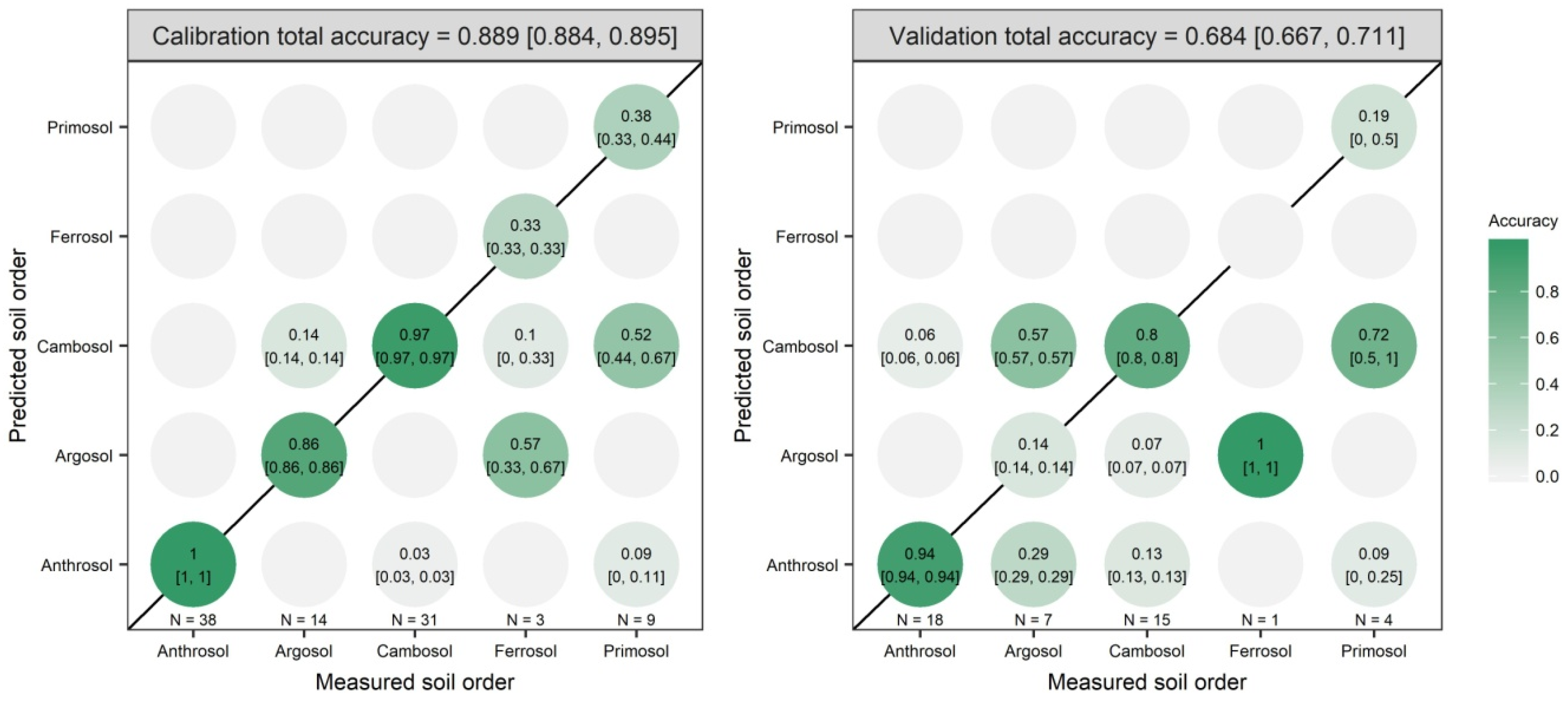
The model performance for vis-NIR spectra revealed total accuracy of 94% with CIs90% between 92.6% and 94.7% in calibration and 64.2% with CIs90% between 62.2% and 66.7% in validation (Figure 5). In calibration, Anthrosols and Argosols had the best classification accuracy, reaching 100%. Cambosols present a high accuracy of 97% (97%, 97%). Ferrosols showed moderate class accuracy of 67% (67%, 67%), and consequently 33% (33%, 33%) were classified as Argosols. In validation, all Ferrosols profiles were classified as Argosols. Anthrosols and Cambosols achieved relatively high accuracy of 89% (89%, 89%) and 73% (73%, 73%), respectively.
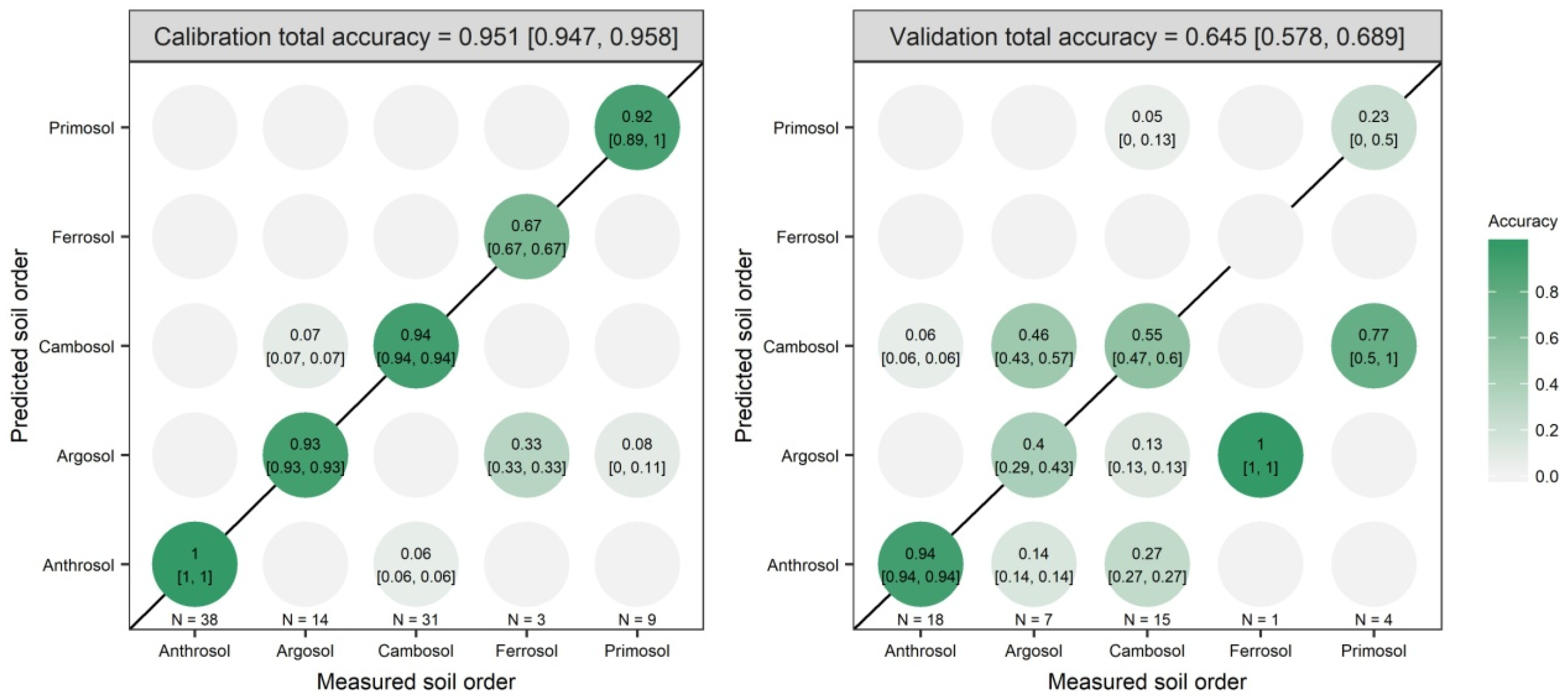
The overall classification accuracy for MIR spectra was 95.1% with CIs90% between 94.7% and 95.8% in calibration and 64.5% with CIs90% between 57.8% and 68.9% in validation (Figure 6). In calibration, except for Ferrosols, the classification accuracies of other soil orders were more than 90%. In validation, the classification results of Ferrosols were similar to those of vis-NIR spectra. Anthrosols had the highest accuracy of 94% (94%, 94%), and they were misclassified as Cambosols. Both Primosols and Argosols present relatively low accuracies of 23% (0%, 50%) and 40% (29%, 43%), respectively.
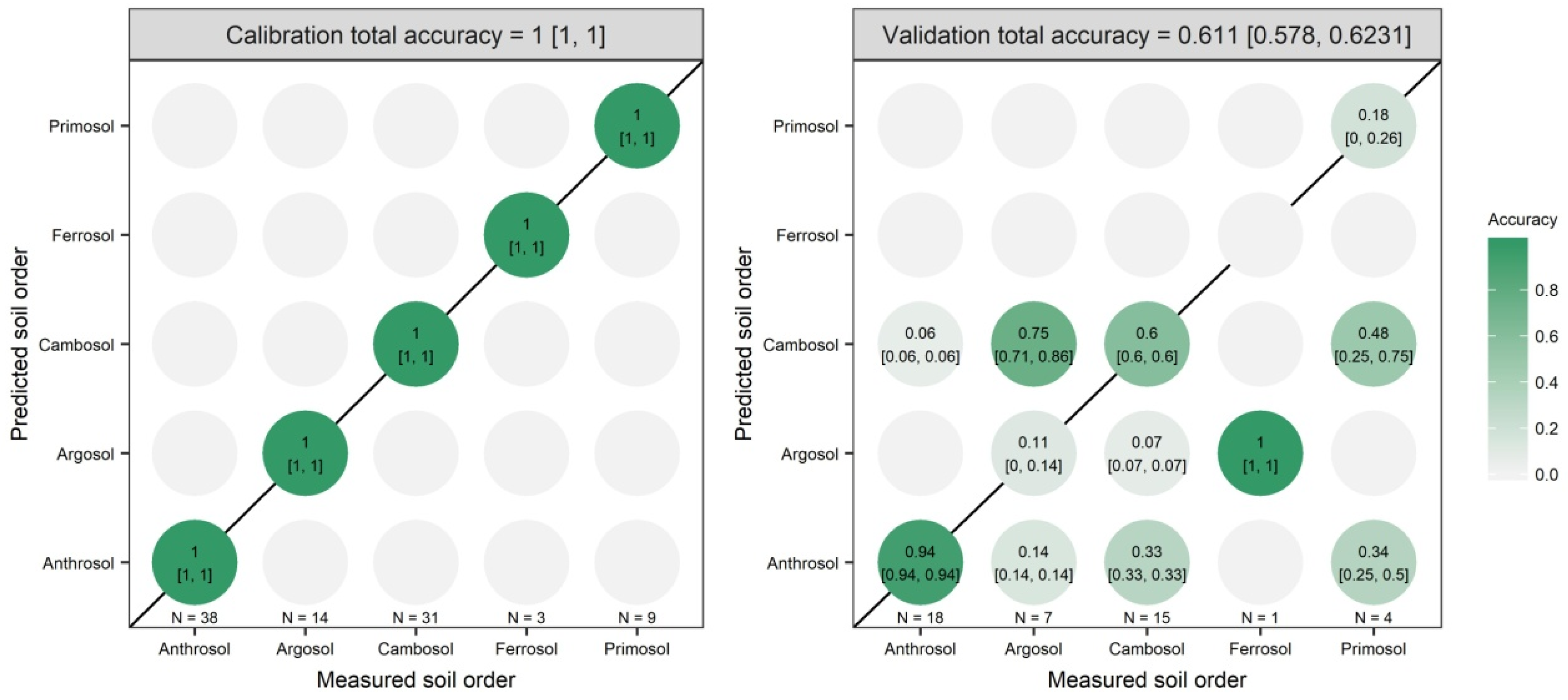
After data fusion, in calibration, the model based on simple spectral combination was correctly classified 100% of the time. In validation, an overall accuracy of 61.1% with CIs90% between 57.8% and 62.31% was obtained (Figure 7). Ferrosols were misclassified completely. Argosols had the second lowest accuracy of 11% (0%, 14%) and was most often misclassified as Cambosols, and the remaining samples were allocated to Anthrosols. Anthrosols showed the highest accuracy of 94% (94%, 94%). Cambosols presented relatively moderate accuracy of 60% (60%, 60%).
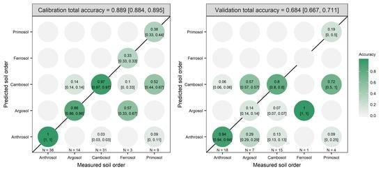
Figure 8 illustrates that the model based on outer product analysis achieved a total accuracy of 88.9% with CIs90% between 88.4% and 89.5% in calibration and 68.4% with CIs90% between 66.7 and 71.1% in validation. The accuracy of validation data using OPA performed the best among the four models. In calibration, all the Anthrosols were correctly classified. Both the Argosols and Cambosols had relatively high accuracies of 86% (86%, 86%) and 97% (97%, 97%), respectively. In validation, Ferrosols failed to be classified once again. In all the models, Ferrosols always achieved 0% and were always misclassified to Argosols. Except for Ferrosols, Argosols were the second misclassified class, of which the accuracy was only 14% (14%, 14%). Cambosols showed relatively high accuracy of 80% (80%, 80%) with a few samples occurring with Argosols and Anthrosols. Similar to the previous models, Anthrosols achieved the highest accuracy of 94% (94%, 94%).
4. Discussion
Soil spectra are able to extract extensive information based on electrical and electromagnetic, optical and radiometric characteristics [33]. This spectra shows the absorption rate of radiation at molecular vibration frequencies. The vibration of these atom groups, such as C-H, N-H, C=O and so on, change the frequency [17]. Previous studies showed the sensitive wave bands of spectral absorption in vis-NIR or MIR for prediction [8]. For vis-NIR spectra, it can contain the information on water (1400, 1900 nm), kaolinite (1400, 2200 nm), illite (2200, 2340, 2445 nm), smectite (2200 nm), carbonate (2335 nm), iron oxides (400, 450, 500, 650, 900 nm) and organic matter (1100, 1600, 1700, 1800, 2000, 2200–2400 nm) [8,57]. For MIR, there are more corresponding sensitive bands than in the vis-NIR regions. For example, under the influence of strong basic group vibration, the sensitive wave bands of SOM in the MIR region (1600–1400, 1630, 1720, 1670, 1530, 2930–2850 cm−1) are more than those in the vis-NIR region [8,58]. On the other hand, overtones and combination bands in vis-NIR region will overlap, and in MIR regions, the peaks would be resolved [21]. Hence, vis-NIR spectra is more difficult to characterize than the MIR spectra [6]. Previous studies showed that the MIR spectra performs better than vis-NIR spectra for predicting some soil properties such as pH, SOM, sand content and so on [6,17,32,57,58]. In contrast, for other properties, such as soil organic carbon, pH, CEC, and total nitrogen, MIR did not perform better than vis-NIR because some useful information might be masked by the strong absorptance of soil minerals [8]. Consequently, it is necessary to combine vis-NIR spectra with MIR spectra for covering as much information as possible.
Table 3 shows the selection of parameters and corresponding prediction accuracy. The results based on MIR spectra (64.5%) are slightly higher than those based on vis-NIR spectra (64.2%). This may occur because spectral modeling based on a single domain would lose soil information due to the heterogeneity of the soil profiles. Thus, we proposed data fusion for soil classification in this study. However, Figure 6 shows that the result based on simple combination was the worst (61.1%), which may be caused by over-fitting in the calibration step. Data fusion via OPA obtained the best classification accuracy (68.4%), though the contribution rate of PCs is lower than that of other models. The simple combination and OPA presents two different levels for data fusion [59]. The simple combination belongs to the low level, which just concatenates spectral data from both sensors. OPA belongs to the high level, which can fuse the features extracted from vis-NIR and MIR [12]. Here, the simple combination achieves worse accuracy than that based on single sensors. The other reason is that spectral data are highly multicollinear. When using both sensors, the spectral data become more redundant and present more noise, which results in decreasing the model stability [59]. Therefore, spectral pre-processing methods play an important role in model prediction when using the simple combination [60]. Although the improvement of classification accuracy by OPA is not that significant (3%), we prove its potential for soil classification with proper pre-processing and a calibration model.
The sample size may be one of the factors affecting classification accuracy. In previous studies, some scholars have further advanced the research that focuses on soil suborder. It is evident that at the soil suborder level, the classification accuracy is significantly decreased [2,45]. When a more detailed soil type is taken into consideration, the sample size is relatively smaller than before. In our study, the accuracy of the classification results is positively correlated with sample size. It can be seen intuitively that Anthrosols with a maximum sample size achieve the highest classification accuracy. Conversely, Ferrosols only contain a few samples. The prediction accuracy of Ferrosols is 0 in each process, obviously. Here, all Ferrosols are misclassified as Argosols, which probably results from data imbalance in the calibration set. That is, the number of Ferrosols is low in the calibration data and thus leads to a small contribution in the calibration model. As for the problem of sample imbalance, it may be solved by a minority oversampling algorithm such as the synthetic minority oversampling technique [61]. Above all, we suggest that sample size is one of the factors affecting the classification accuracy, and the sample size differences of each class lead to sample imbalance while modeling. The establishment of soil spectral libraries across scales may be a good solution to further improve accuracy of soil classification [11,62,63].
For classification of each soil order, it is necessary to find a general pattern in the misclassification. In calibration, the misclassification of Ferrosols is predominantly observed with Argosols. We have mentioned before that the main diagnostic characteristics of Argosols are argic horizon, kandic horizon, natric horizon, and clay pan. The main diagnostic characteristics of Ferrosols are allitization and ferritization. Both of these genesis processes lead to soil clay accumulation and strong base eluviation, which makes the soil texture similar. For Argosols, most of errors are re-allocated to Cambosols. The diagnostic characteristics of Cambosols are a cambic horizon, whose soil structure is preliminarily formed without significant clayification and illuviation. Comparing Cambosols with Argosols, there is almost no correlation between their diagnostic characteristics. We found that soil properties of different classes or horizons do not show significant differences, and the spectra curves of some soil classes also overlap [11,43], either of which might cause the misclassification. For Primosols, most of the errors occur with Cambosols. The genesis process may explain the error. Primosols are less profile developed and have no diagnostic horizon and characteristic. With a short history of development, the weathering and pedogenesis of both of profiles are weak. Moreover, comparing Anthrosols with Cambosols, both of them achieve high accuracy. The accuracy of Anthrosols reaches nearly 100%. Only a few of the samples are misclassified as Cambosols in the validation process. However, the diagnostic horizon and characteristics between them are totally different. As mentioned above, both have relatively large proportions in calibration data. The calibration model will learn more and cover more features. These results might also explain the reason why most misclassifications were classified as Anthrosols and Cambosols.
In this study, we tried to optimize the gamma and cost parameters to improve the model. We determined the ranges of gamma and cost by expert knowledge. Actually, the parameter selection ranges are infinite. Future studies could focus on finding a better solution for parameter selection (or grid search) out of the range determined in this study.
The soil profiles used in this study only cover 5 soil orders, while other soil orders are still missing. This is because soil order is the highest classification level, which ensures enough data for classification. With the limited sample size, there are no studies focusing on classifying soil group, soil subgroup and soil series. To build a robust classification model at these levels, more soil profile data are needed. Therefore, if the number of samples is large enough and covers as widely as possible, models will perform better, and the classification accuracy will be significantly improved. Although it is time and cost consuming to collect more soil profile data, we will continue to expand our soil database and to improve the model. With continuous data collection, the database and model can be updated constantly. It is worth noting that in the update process, the sample treatment process and analysis should be as consistent as possible [43].
Apart from sample size, model parameter and characteristics of soil profile itself, the limitations of the spectra itself is another factor influencing the accuracy of soil classification. As we know, the processes of pedogenesis and soil development are extremely complex. The processes are affected by climate, biology, parent material, topography, time, and man-made factors. In the process of soil formation, interaction with the surrounding environment will be involved. The interaction of the geological cycle and the biological cycle is the basis of soil genesis. Under the action of soil forming factors, a series of soil physical, chemical, and biological characteristics are developed, thus leading to different soil types. Therefore, most current adopted soil classification is based on the theory of soil genesis and soil characteristics. [64]. It is the same case in China that CST uses diagnostic horizons and diagnostic characteristics as the core of soil classification. In this study, we obtained the soil property data and spectral data quantitatively at each horizon. Although quantitative data can guarantee the objectivity of classification [50], these quantitative data cannot well reflect all the diagnostic horizons and diagnostic characteristics. For instance, the main diagnostic characteristics of Ferrosols and Argosols are ferritization and clay pans, respectively. Though previous studies indicated a high prediction accuracy for clay contents and iron oxide contents by vis-NIR and MIR [6,20,49], we cannot infer that vis-NIR and MIR are able to predict clay pans and ferritization. Moreover, even for these well predicted soil properties (e.g., SOC, clay), there is still a large prediction uncertainty. Considering the comprehensive framework involved in soil classification, classification error occurs if we only simply use these soil properties.
Meanwhile, soil spectral data may ignore the information relevant to soil genesis. In the study of soil genesis, whether the homology or heterogeneity of parent material is clear can help us better understand and distinguish the real causes of the change trend of soil properties. For the soil genesis process, discontinuity of parent material is universal. However, it is not easy to determine the discontinuity of parent material. When there are obvious differences in soil texture and structure in profile morphology, the discrimination of discontinuity of parent material is easier. However it is difficult to identify it if the profile features are uniform. Previous studies discussed some solutions, such as deep functions, uniformity value, and discriminant analysis [65]; while all of them have their limitations and need to be improved. In our study, although soil spectra is able to provide information related to soil properties, it cannot well capture all the relevant diagnostic characteristics. Overall, due to its limitations, soil spectroscopy cannot fully replace conventional soil classification, but it has a high potential to aid soil classification once the soil spectral libraries are well established. It also should be noted that the prediction of soil classification based on soil spectra still remains an academic research topic and more efforts should be pursued for its practical use in decision making for farmers and stakeholders.
5. Conclusions
We used data fusion for soil classification. There were four models constructed in our study as follows: (1) a model based on vis-NIR, (2) a model based on MIR, (3) a model based on simple spectral combination and (4) a model based on OPA. For single domains, the models based on vis-NIR (64.2%) and MIR (64.5%) show similar results. For data fusion, the model based on spectral combination performs worse (61.1%) than that based on single domains. The model based on OPA performs best (68.4%). It shows that soil classification using data fusion could improve accuracy.
Author Contributions
Conceptualization, Z.S., S.C. and D.X.; methodology, S.C. and D.X.; software, H.X.; validation, H.X.; formal analysis, H.X.; investigation, W.M.; resources, W.M.; data curation, W.M.; writing—original draft preparation, H.X.; writing—review and editing, D.X. and S.C; visualization, H.X.; supervision, D.X. and Z.S.; project administration, Z.S.; funding acquisition, Z.S. All authors have read and agreed to the published version of the manuscript.
Funding
This research was funded by National Key Research and Development Program (2018YFE0107000); Public Welfare Research of Zhejiang Province (LGN18D010003).
Acknowledgments
The authors’ great gratitude is extended to Zhejiang Academy of Agricultural Sciences for data acquisition and provision.
Conflicts of Interest
The authors declare no conflict of interest.
References
- McBratney, A.B.; Odeh, I.O.A.; Bishop, T.F.A.; Dunbar, M.S.; Shatar, T.M. An overview of pedometric techniques for use in soil survey. Geoderma 2000, 97, 293–327. [Google Scholar] [CrossRef]
- Vasques, G.M.; Dematte, J.A.M.; Viscarra Rossel, R.A.; Ramirez-Lopez, L.; Terra, F.S. Soil classification using visible/near-infrared diffuse reflectance spectra from multiple depths. Geoderma 2014, 223, 73–78. [Google Scholar] [CrossRef]
- Craswell, E.T.; Lefroy, R.D.B. The role and function of organic matter in tropical soils. Nutr. Cycl. Agroecosyst. 2001, 61, 7–18. [Google Scholar] [CrossRef]
- McCarty, G.W.; Reeves, J.B.; Reeves, V.B.; Follett, R.F.; Kimble, J.M. Mid-infrared and near-infrared diffuse reflectance spectroscopy for soil carbon measurement. Soil Sci. Soc. Am. J. 2002, 66, 640–646. [Google Scholar]
- Nocita, M.; Stevens, A.; van Wesemael, B.; Aitkenhead, M.; Bachmann, M.; Barthes, B.; Ben Dor, E.; Brown, D.J.; Clairotte, M.; Csorba, A.; et al. Soil Spectroscopy: An alternative to wet chemistry for soil monitoring. Adv. Agron. 2015, 132, 139–159. [Google Scholar]
- Viscarra Rossel, R.A.; Walvoort, D.J.J.; McBratney, A.B.; Janik, L.J.; Skjemstad, J.O. Visible, near infrared, mid infrared or combined diffuse reflectance spectroscopy for simultaneous assessment of various soil properties. Geoderma 2006, 131, 59–75. [Google Scholar] [CrossRef]
- Stenberg, B.; Viscarra Rossel, R.A.; Mouazen, A.M.; Wetterlind, J. Visible and near infrared spectroscopy in soil science. Adv. Agron. 2010, 107, 163–215. [Google Scholar]
- Soriano-Disla, J.M.; Janik, L.J.; Viscarra Rossel, R.A.; Macdonald, L.M.; McLaughlin, M.J. The performance of visible, near-, and mid-infrared reflectance spectroscopy for prediction of soil physical, chemical, and biological properties. Appl. Spectrosc. Rev. 2014, 49, 139–186. [Google Scholar] [CrossRef]
- Ji, W.; Li, S.; Chen, S.; Shi, Z.; Viscarra Rossel, R.A.; Mouazen, A.M. Prediction of soil attributes using the Chinese soil spectral library and standardized spectra recorded at field conditions. Soil Tillage Res. 2016, 155, 492–500. [Google Scholar] [CrossRef]
- Bilgili, A.V.; van Es, H.M.; Akbas, F.; Durak, A.; Hively, W.D. Visible-near infrared reflectance spectroscopy for assessment of soil properties in a semi-arid area of Turkey. J. Arid Environ. 2010, 74, 229–238. [Google Scholar] [CrossRef]
- Shi, Z.; Wang, Q.; Peng, J.; Ji, W.; Liu, H.; Li, X.; Viscarra Rossel, R.A. Development of national VNIR soil-spectral library for soil classification and the predictions of organic matter. Sci. China Earth Sci. 2014, 57, 1671–1680. [Google Scholar] [CrossRef]
- Ng, W.; Minasny, B.; Montazerolghaem, M.; Padarian, J.; Ferguson, R.; Bailey, S.; McBratney, A.B. Convolutional neural network for simultaneous prediction of several soil properties using visible/near-infrared, mid-infrared, and their combined spectra. Geoderma 2019, 352, 251–267. [Google Scholar] [CrossRef]
- Shepherd, K.D.; Walsh, M.G. Development of reflectance spectral libraries for characterization of soil properties. Soil Sci. Soc. Am. J. 2002, 66, 988–998. [Google Scholar] [CrossRef]
- Islam, K.; Singh, B.; McBratney, A. Simultaneous estimation of several soil properties by ultra-violet, visible, and near-infrared reflectance spectroscopy. Aust. J. Soil Res. 2003, 41, 1101–1114. [Google Scholar] [CrossRef]
- McDowell, M.L.; Bruland, G.L.; Deenik, J.L.; Grunwald, S.; Knox, N.M. Soil total carbon analysis in Hawaiian soils with visible, near-infrared and mid-infrared diffuse reflectance spectroscopy. Geoderma 2012, 189–190, 312–320. [Google Scholar] [CrossRef]
- Dematte, J.A.M.; Terra, F.D. Spectral pedology: A new perspective on evaluation of soils along pedogenetic alterations. Geoderma 2014, 217, 190–200. [Google Scholar] [CrossRef]
- Yang, M.H.; Xu, D.Y.; Chen, S.C.; Li, H.Y.; Shi, Z. Evaluation of Machine Learning Approaches to Predict Soil Organic Matter and pH Using vis-NIR Spectra. Sensors 2019, 19, 263. [Google Scholar] [CrossRef] [Green Version]
- Chang, C.W.; Laird, D.A. Near-infrared reflectance spectroscopic analysis of soil C and N. Soil Sci. 2002, 167, 110–116. [Google Scholar] [CrossRef]
- Cozzolino, D.; Moron, A. The potential of near-infrared reflectance spectroscopy to analyse soil chemical and physical characteristics. J. Agric. Sci. 2003, 140, 65–71. [Google Scholar] [CrossRef]
- Terra, F.S.; Dematte, J.A.M.; Viscarra Rossel, R.A. Proximal spectral sensing in pedological assessments: Vis-NIR spectra for soil classification based on weathering and pedogenesis. Geoderma 2018, 318, 123–136. [Google Scholar] [CrossRef]
- Janik, L.J.; Merry, R.H.; Skjemstad, J.O. Can mid infra-red diffuse reflectance analysis replace soil extractions? Aust. J. Exp. Agric. 1998, 38, 681–696. [Google Scholar] [CrossRef]
- Reeves, J.B., III. Near- versus mid-infrared diffuse reflectance spectroscopy for soil analysis emphasizing carbon and laboratory versus on-site analysis: Where are we and what needs to be done? Geoderma 2010, 158, 3–14. [Google Scholar] [CrossRef]
- Terra, F.S.; Dematte, J.A.M.; Viscarra Rossel, R.A. Spectral libraries for quantitative analyses of tropical Brazilian soils: Comparing vis-NIR and mid-IR reflectance data. Geoderma 2015, 255, 81–93. [Google Scholar] [CrossRef]
- Wang, S.; Li, W.; Li, J.; Liu, X. Prediction of soil texture using FT-NIR spectroscopy and PXRF spectrometry with data fusion. Soil Sci. 2013, 178, 626–638. [Google Scholar] [CrossRef]
- Aldabaa, A.A.A.; Weindorf, D.C.; Chakraborty, S.; Sharma, A.; Li, B. Combination of proximal and remote sensing methods for rapid soil salinity quantification. Geoderma 2015, 239, 34–46. [Google Scholar] [CrossRef] [Green Version]
- O’Rourke, S.M.; Stockmann, U.; Holden, N.M.; McBratney, A.B.; Minasny, B. An assessment of model averaging to improve predictive power of portable vis-NIR and XRF for the determination of agronomic soil properties. Geoderma 2016, 279, 31–44. [Google Scholar] [CrossRef]
- Xu, D.; Chen, S.; Viscarra Rossel, R.A.; Biswas, A.; Li, S.; Zhou, Y.; Shi, Z. X-ray fluorescence and visible near infrared sensor fusion for predicting soil chromium content. Geoderma 2019, 352, 61–69. [Google Scholar] [CrossRef]
- Xu, D.; Zhao, R.; Li, S.; Chen, S.; Jiang, Q.; Zhou, L.; Shi, Z. Multi-sensor fusion for the determination of several soil properties in the Yangtze River Delta, China. Eur. J. Soil Sci. 2019, 70, 162–173. [Google Scholar] [CrossRef] [Green Version]
- Wang, D.; Chakraborty, S.; Weindorf, D.C.; Li, B.; Sharma, A.; Paul, S.; Ali, M.N. Synthesized use of VisNIR DRS and PXRF for soil characterization: Total carbon and total nitrogen. Geoderma 2015, 243, 157–167. [Google Scholar] [CrossRef]
- Terra, F.S.; Viscarra Rossel, R.A.; Dematte, J.A.M. Spectral fusion by Outer Product Analysis (OPA) to improve predictions of soil organic C. Geoderma 2019, 335, 35–46. [Google Scholar] [CrossRef]
- Chakraborty, S.; Weindorf, D.C.; Li, B.; Ali Aldabaa, A.A.; Ghosh, R.K.; Paul, S.; Nasim Ali, M. Development of a hybrid proximal sensing method for rapid identification of petroleum contaminated soils. Sci. Total Environ. 2015, 514, 399–408. [Google Scholar] [CrossRef] [PubMed]
- O’Rourke, S.M.; Minasny, B.; Holden, N.M.; McBratney, A.B. Synergistic use of vis-NIR, MIR, and XRF spectroscopy for the determination of soil geochemistry. Soil Sci. Soc. Am. J. 2016, 80, 888–899. [Google Scholar] [CrossRef] [Green Version]
- Ji, W.; Adamchuk, V.I.; Chen, S.; Su, A.S.M.; Ismail, A.; Gan, Q.; Shi, Z.; Biswas, A. Simultaneous measurement of multiple soil properties through proximal sensor data fusion: A case study. Geoderma 2019, 341, 111–128. [Google Scholar] [CrossRef]
- Condit, H.R. The spectral reflectance of American soils. Photogramm. Eng. 1970, 36, 955–966. [Google Scholar]
- Cipra, J.E.; Stoner, E.R.; Baumgardner, M.F.; Macdonald, R.B. Measuring radiance characteristics of soil with a spectroradiometer. Soil Sci. Soc. Am. Proc. 1971, 35, 1014–1017. [Google Scholar] [CrossRef]
- Stoner, E.R.; Baumgardner, M.F. Characteristic variations in reflectance of surface soils. Soil Sci. Soc. Am. J. 1981, 45, 1161–1165. [Google Scholar] [CrossRef] [Green Version]
- Wang, R.C.; Su, H.P.; Wang, S.F. Studies on spectral reflectance of typical soils and its fuzzy category in soil classification in Zhejiang province. J. Zhejiang Univ. Sci. B 1986, 12, 464–471. [Google Scholar]
- Xu, B.B. Research of China’s soil spectral line. J. Remote Sens. 1991, 1, 61–71. [Google Scholar]
- Ji, W.J.; Shi, Z.; Zhou, Q.; Zhou, L.Q. VIS-NIR reflectance spectroscopy of the organic matter in several types of soils. J. Infrared Millim. Terahertz Waves 2012, 31, 277–282. [Google Scholar] [CrossRef]
- Linker, R. Soil classification via mid-infrared spectroscopy. In Computer and Computing Technologies in Agriculture; Springer: New York, NY, USA, 2008; Volume 259, pp. 1137–1146. [Google Scholar]
- Mouazen, A.M.; Karoui, R.; De Baerdemaeker, J.; Ramon, H. Classification of soil texture classes by using soil visual near infrared spectroscopy and factorial discriminant analysis techniques. J. Near Infrared Spectrosc. 2005, 13, 231–240. [Google Scholar] [CrossRef]
- Oliveira, J.F.; Brossard, M.; Siqueira Vendrame, P.R.; Mayi, S., III; Corazza, E.J.; Marchao, R.L.; Guimaraes, M.d.F. Soil discrimination using diffuse reflectance Vis-NIR spectroscopy in a local toposequence. Comptes Rendus Geosci. 2013, 345, 446–453. [Google Scholar] [CrossRef]
- Teng, H.; Viscarra Rossel, R.A.; Shi, Z.; Behrens, T. Updating a national soil classification with spectroscopic predictions and digital soil mapping. Catena 2018, 164, 125–134. [Google Scholar] [CrossRef]
- Viscarra Rossel, R.A.; Webster, R. Discrimination of Australian soil horizons and classes from their visible-near infrared spectra. Eur. J. Soil Sci. 2011, 62, 637–647. [Google Scholar] [CrossRef]
- Chen, S.; Li, S.; Ma, W.; Ji, W.; Xu, D.; Shi, Z.; Zhang, G. Rapid determination of soil classes in soil profiles using vis-NIR spectroscopy and multiple objectives mixed support vector classification. Eur. J. Soil Sci. 2019, 70, 42–53. [Google Scholar] [CrossRef] [Green Version]
- Dotto, A.; Demattê, J.; Viscarra Rossel, R.A.; Rizzo, R. Soil classification based on spectral and environmental variables. SOIL Dis. 2019, 1–20. [Google Scholar] [CrossRef]
- Shi, X.Z.; Yu, D.S.; Yang, G.X.; Wang, H.J.; Sun, W.X.; Du, G.H.; Gong, Z.T. Cross-reference benchmarks for translating the Genetic Soil Classification of China into the Chinese Soil Taxonomy. Pedosphere 2006, 16, 147–153. [Google Scholar] [CrossRef]
- IUSS Working Group WRB. World Reference Base for Soil Resources 2014, Update 2015 International Soil Classification System for Naming Soils and Creating Legends for Soil Maps. World Soil Resour. Rep. 2015, 106, 192. [Google Scholar]
- Xu, D.; Ma, W.; Chen, S.; Jiang, Q.; He, K.; Shi, Z. Assessment of important soil properties related to Chinese Soil Taxonomy based on vis-NIR reflectance spectroscopy. Comput. Electron. Agric. 2018, 144, 1–8. [Google Scholar] [CrossRef]
- Institute of Soil Science, Chinese Academy of Sciences. Chinese Soil Taxonomy, 1st ed.; China Agricultural Science and Technology Press: Beijing, China, 1995; pp. 19–37. [Google Scholar]
- Beaudette, D.E.; Roudier, P.; O’Geen, A.T. Algorithms for quantitative pedology: A toolkit for soil scientists. Comput. Geosci. 2013, 52, 258–268. [Google Scholar] [CrossRef]
- The R Development Core Team. In R: A Language and Environment for Statistical Computing; R Foundation for Statistical Computing: Vienna, Austria, 2015.
- Barros, A.S.; Safar, M.; Devaux, M.F.; Robert, P.; Bertrand, D.; Rutledge, D.N. Relations between mid-infrared and near-infrared spectra detected by analysis of variance of an intervariable data matrix. Appl. Spectrosc. 1997, 51, 1384–1393. [Google Scholar] [CrossRef]
- Jaillais, B.; Ottenhof, M.A.; Farhat, I.A.; Rutledge, D.N. Outer-product analysis (OPA) using PLS regression to study the retrogradation of starch. Vib. Spectrosc. 2006, 40, 10–19. [Google Scholar] [CrossRef]
- Joachims, T. Text categorization with support vector machines: Learning with many relevant features. In Proceedings of the European Conference on Machine Learning, Berlin/Heidelberg, Germany, 21–23 April 1998; Springer: Berlin/Heidelberg, Germany. [Google Scholar]
- Hsu, C.W.; Lin, C.J. A comparison of methods for multiclass support vector machines. IEEE Trans. Neural Netw. 2002, 13, 415–425. [Google Scholar] [PubMed] [Green Version]
- Li, S.; Ji, W.; Chen, S.; Peng, J.; Zhou, Y.; Shi, Z. Potential of VIS-NIR-SWIR spectroscopy from the Chinese soil spectral library for assessment of nitrogen fertilization rates in the paddy-rice region, China. Remote Sens. 2015, 7, 7029–7043. [Google Scholar] [CrossRef] [Green Version]
- Chen, S.C.; Peng, J.; Ji, W.J.; Zhou, Y.; He, J.X.; Shi, Z. Study on the characterization of VNIR-MIR spectra and prediction of soil organic matter in paddy soil. Spectrosc. Spect. Anal. 2016, 36, 1712–1716. [Google Scholar]
- Borras, E.; Ferre, J.; Boque, R.; Mestres, M.; Acena, L.; Busto, O. Data fusion methodologies for food and beverage authentication and quality assessment—A review. Anal. Chim. Acta 2015, 891, 1–14. [Google Scholar] [CrossRef]
- Knox, N.M.; Grunwald, S.; McDowell, M.L.; Bruland, G.L.; Myers, D.B.; Harris, W.G. Modelling soil carbon fractions with visible near-infrared (VNIR) and mid-infrared (MIR) spectroscopy. Geoderma 2015, 239, 229–239. [Google Scholar] [CrossRef]
- Chawla, N.; Bowyer, K.; Hall, L.; Kegelmeyer, W. SMOTE: Synthetic minority over-sampling technique. J. Artif. Intell. Res. 2002, 16, 321–357. [Google Scholar] [CrossRef]
- Viscarra Rossel, R.A.; Behrens, T.; Ben-Dor, E.; Brown, D.J.; Dematte, J.A.M.; Shepherd, K.D.; Shi, Z.; Stenberg, B.; Stevens, A.; Adamchuk, V.; et al. A global spectral library to characterize the world’s soil. Earth-Sci. Rev. 2016, 155, 198–230. [Google Scholar] [CrossRef] [Green Version]
- Stevens, A.; Nocita, M.; Toth, G.; Montanarella, L.; van Wesemael, B. Prediction of soil organic carbon at the european scale by visible and near infrared reflectance spectroscopy. PLoS ONE 2013, 8, 13. [Google Scholar] [CrossRef]
- Huang, C.Y.; Xu, J.M. Pedology, 3rd ed.; China Agriculture Press: Beijing, China, 2011; pp. 80–107, 293–308. [Google Scholar]
- Chen, L.M.; Zhang, G.L. Soil chronosequences and the significance in the study of pedogenesis. Acta Pedol. Sin. 2011, 48, 421–428. [Google Scholar]
Figure 1.
Location of the study area and the sampling sites of soil profiles.

Figure 2.
Workflow of data fusion by outer product analysis (OPA) (revised after [27]).
Figure 2.
Workflow of data fusion by outer product analysis (OPA) (revised after [27]).

Figure 3.
Workflow in this study.

Figure 4.
Violin plots of different soil profiles. The median values of each soil order are indicated by the numbers inside each violin: (a) soil organic matter, (b) sand, (c) silt, and (d) clay. The numbers shown inside each violin are the median values of each soil order.
Figure 4.
Violin plots of different soil profiles. The median values of each soil order are indicated by the numbers inside each violin: (a) soil organic matter, (b) sand, (c) silt, and (d) clay. The numbers shown inside each violin are the median values of each soil order.

Figure 5.
Confusion matrix of soil classification based on vis–NIR spectra. Inside the square brackets are lower and upper limits of the 90% confidence intervals. Outside are mean values. N represents the number of samples in each soil order allocated by model.
Figure 5.
Confusion matrix of soil classification based on vis–NIR spectra. Inside the square brackets are lower and upper limits of the 90% confidence intervals. Outside are mean values. N represents the number of samples in each soil order allocated by model.

Figure 6.
Confusion matrix of soil classification based on MIR spectra.

Figure 7.
Confusion matrix of soil classification based on spectral combination.

Figure 8.
Confusion matrix of soil classification based on outer product analysis.


Table 1.
Soil orders and suborders classified for 146 soil profiles.
| Soil Order | Soil Suborder | Numbers of Samples |
|---|---|---|
| Anthrosol | Stagnic Anthrosol | 54 |
| Orthic Anthrosol | 2 | |
| Halosol | Orthic Halosol | 2 |
| Gleyosol | Stagnic Gleyosol | 1 |
| Isohumosol | Udic Isohumosol | 2 |
| Ferrosol | Udic Ferrosol | 4 |
| Argosol | Udic Argosol | 21 |
| Cambosol | Aquic Cambosol | 16 |
| Perudic Cambosol | 6 | |
| Udic Cambosol | 24 | |
| Primosol | Alluvic Primosol | 6 |
| Orthic Primosol | 6 | |
| Anthric Primosol | 1 |
Table 2.
Correlation between the Chinese Soil Taxonomy (CST) and the World Reference Base on the soil order level [48].
Table 2.
Correlation between the Chinese Soil Taxonomy (CST) and the World Reference Base on the soil order level [48].
| Chinese Soil Taxonomy | World Reference Base |
|---|---|
| Cambosols | Cambisols |
| Argosols | Luvisols, Alisols |
| Gleyosols | Gleysols, Cryosols |
| Primosols | Fluvisols, Leptisols, Arenosols, Regosols, Cryosols |
| Halosols | Solonchaks, Solonetz |
| Isohumosols | Chernozems, Kastanozems, Phaeozems |
| Anthrosols | Anthrosols |
| Ferrosols | Acrisols, Lixisols, Plinthosols, Nitisols |
Table 3.
Parameter optimization for a support vector machine (SVM) and prediction result statistics for calibration and validation sets.
Table 3.
Parameter optimization for a support vector machine (SVM) and prediction result statistics for calibration and validation sets.
| Method | PCs Selection | Contribution Rate/% | Optimal Parameters | Total Accuracy | ||
|---|---|---|---|---|---|---|
| Gamma | Cost | Calibration | Validation | |||
| Vis-NIR | PC1 to PC20 | 99.8 | 0.025 | 1 | 0.94 | 0.642 |
| MIR | PC1 to PC40 | 99.76 | 0.0125 | 1.5 | 0.951 | 0.645 |
| Combination | PC1 to PC50 | 99.5 | 0.025 | 2.5 | 1 | 0.611 |
| OPA | PC1 to PC20 | 98.99 | 0.0625 | 0.5 | 0.889 | 0.684 |
© 2020 by the authors. Licensee MDPI, Basel, Switzerland. This article is an open access article distributed under the terms and conditions of the Creative Commons Attribution (CC BY) license (http://creativecommons.org/licenses/by/4.0/).
Share and Cite
MDPI and ACS Style
Xu, H.; Xu, D.; Chen, S.; Ma, W.; Shi, Z. Rapid Determination of Soil Class Based on Visible-Near Infrared, Mid-Infrared Spectroscopy and Data Fusion. Remote Sens. 2020, 12, 1512. https://doi.org/10.3390/rs12091512
AMA Style
Xu H, Xu D, Chen S, Ma W, Shi Z. Rapid Determination of Soil Class Based on Visible-Near Infrared, Mid-Infrared Spectroscopy and Data Fusion. Remote Sensing. 2020; 12(9):1512. https://doi.org/10.3390/rs12091512
Chicago/Turabian StyleXu, Hanyi, Dongyun Xu, Songchao Chen, Wanzhu Ma, and Zhou Shi. 2020. "Rapid Determination of Soil Class Based on Visible-Near Infrared, Mid-Infrared Spectroscopy and Data Fusion" Remote Sensing 12, no. 9: 1512. https://doi.org/10.3390/rs12091512
Note that from the first issue of 2016, this journal uses article numbers instead of page numbers. See further details here.