Article

Can Commercial Low-Cost Drones and Open-Source GIS Technologies Be Suitable for Semi-Automatic Weed Mapping for Smart Farming? A Case Study in NE Italy

by
Pietro Mattivi
1,
Salvatore Eugenio Pappalardo
2,*,
Nebojša Nikolić
3,
Luca Mandolesi
4,
Antonio Persichetti
5,
Massimo De Marchi
2 and
Roberta Masin
3
1
Department of Civil, Chemical, Environmental and Materials Engineering—DICAM, University of Bologna, 40136 Bologna, Italy
2
Department of Civil, Environmental and Architectural Engineering—ICEA, University of Padua, 35100 Padova, Italy
3
Department of Agronomy, Food, Natural Resources, Animals and Environment—DAFNAE, University of Padova, 35020 Legnaro, Italy
4
AdArte, 47921 Rimini, Italy
5
Archetipo s.r.l., 35129 Padova, Italy
*
Author to whom correspondence should be addressed.
Remote Sens. 2021, 13(10), 1869; https://doi.org/10.3390/rs13101869
Submission received: 14 March 2021 / Revised: 1 May 2021 / Accepted: 6 May 2021 / Published: 11 May 2021
(This article belongs to the Special Issue Precision Weed Mapping and Management Based on Remote Sensing)

Abstract

:
Weed management is a crucial issue in agriculture, resulting in environmental in-field and off-field impacts. Within Agriculture 4.0, adoption of UASs combined with spatially explicit approaches may drastically reduce doses of herbicides, increasing sustainability in weed management. However, Agriculture 4.0 technologies are barely adopted in small-medium size farms. Recently, small and low-cost UASs, together with open-source software packages, may represent a low-cost spatially explicit system to map weed distribution in crop fields. The general aim is to map weed distribution by a low-cost UASs and a replicable workflow, completely based on open GIS software and algorithms: OpenDroneMap, QGIS, SAGA and OpenCV classification algorithms. Specific objectives are: (i) testing a low-cost UAS for weed mapping; (ii) assessing open-source packages for semi-automatic weed classification; (iii) performing a sustainable management scenario by prescription maps. Results showed high performances along the whole process: in orthomosaic generation at very high spatial resolution (0.01 m/pixel), in testing weed detection (Matthews Correlation Coefficient: 0.67–0.74), and in the production of prescription maps, reducing herbicide treatment to only 3.47% of the entire field. This study reveals the feasibility of low-cost UASs combined with open-source software, enabling a spatially explicit approach for weed management in small-medium size farmlands.

1. Introduction

1.1. A Spatial Approach for Weed Management in Smart Farming

Farmland weeds are a common issue both in conventional and organic farming. Due to their competitiveness and fast spreading, weed control is required to maintain quantity and quality of crop production [1,2,3]. For this purpose, numerous weed management options have been developed in agriculture, including mechanical, chemical, agronomical and physical methods [4,5,6,7]. Among these, mechanical and chemical methods are the most widespread, with the latter being also the most effective as the herbicides provoke plant decay and death [5,8,9]. Other mentioned methods cannot be effectively used on their own but instead as part of a holistic weed control system [10,11]. Although being the two mostly used weed controlling methods, mechanical and chemical management both present some constraints. The first one can cause several negative effects for the soil (compaction, soil erosion, fertility reduction, etc.), and the second one can seriously affect the environment, including soil and water biota as well as human health [12,13,14,15]. Taking this into account, inappropriate weed management, both at field and territory scale, can be environmentally and economically unsustainable. In fact, weed treatments represent potential ecological impacts both in terms of in-field/out-field chemical pollution and, in addition to mechanical weed control measures, the means for herbicide application could be an indirect driver of soil compaction and erosion [16,17]. In Europe, the cost of herbicides is equal to the 40% of the total cost of all the chemicals adopted in agrosystems management. All these concerns led to the creation of the European legislation framework on the sustainable use of pesticides, driving technologies and new agronomic practices within the new framework of Agriculture 4.0 by adopting Precision Agriculture Technologies (PAT). One of the promising practices which increase sustainability of weed management is based on the so-called Site-Specific Weed Management (SSWM) strategies [18,19]. In fact, the ecological impacts of herbicides are generally the consequence of three main critical issues in weed management: (i) the application of herbicide during an inappropriate weed phenological stage; (ii) the lack of weed threshold assessment in terms of degree of infestation; (iii) the application of herbicides over the entire field, without considering the weed spatial distribution [20,21,22,23]. While the first depends on experiences and agronomic knowledge of the farmer, the latter could be addressed by developing SSWM strategies. Such agronomic strategies can lead to: (i) a relevant reduction of environmental impacts on soil, and surface and shallow water bodies; (ii) a decrease of weed management costs for herbicides; (iii) compliance with the European legislation on the use of pesticides [17,18,24,25,26,27].
A SSWM requires the use of adequate doses of herbicide in the areas of the field where the degree of infestation exceeds a certain threshold. As a result, spatially-based treatments are customized for every specific case, according to the distribution of weeds [19,28].
As well documented, weeds are non-uniformly distributed at any spatial scale; therefore, within a field, their distribution is quite heterogeneous and irregular [29]. For this reason, the SSWM adopts a spatially-explicit approach to identify weed distribution in order to generate site-specific herbicide application maps. Thus, it is necessary to identify weed distribution at field scale, in order to spatially assess the weed coverage density and, therefore, to generate treatment maps [17,19,30]. In the past, weed distribution assessment was usually performed by direct observations and by scouting through the crop field, making this task extremely time and resource consuming and not very reliable [31]. Since spatial patterns of weeds usually appear in patches, data acquisition by aerial surveys currently represents an important opportunity to identify and to map infested areas within the crop [32,33].

1.2. Unmanned Aerial Systems for Weed Detection

In recent years, the use of remote sensing together with machine vision techniques has notably increased, making geospatial technologies a potential tool to precisely and automatically detect weeds [34,35,36,37]. Due to their spatial resolutions, ranging from 30 to 0.2 m per pixel, aircraft and satellite images are generally not suitable for field-scale weed mapping. Therefore, the rapid and extensive spreading of Unmanned Aerial Systems (UASs) currently represents a promising technology for weed identification and management [29,38,39]. In fact, UAS can fly at lower altitudes, considerably increasing spatial resolution up to 0.01 m per pixel. Furthermore, UAS can be equipped with different kinds of sensors (from optical to multi- and hyper-spectral sensors) and they can operate on demand for weed detection and management, giving an integrated technical and operative support to precision farming for Agriculture 4.0. However, probably due to the effort in investments as well as lack in knowledge and technology transfer, UAS and geospatial approaches seems to be less attractive for small-medium farms, which currently represent a relevant part of agricultural land worldwide.
To fill this gap, an opportunity window is today represented by the spread of commercial small and low-cost UASs which may bring also to small-medium farms a spatially-based weed management agronomic practice at field scale. In fact, low-cost UASs are usually equipped with very high-resolution sensors supporting RGB bands in the visible spectral range. Most diffused low-cost UAS sensors range from 2/3 to 1” CMOS size, with 12–20 million pixels. Therefore, low-cost UASs seem suitable for weed detection compared to other remote sensing aerial platforms, field surveys, or other conventional techniques [17,19,29].
In addition, the continuous development of new tools and techniques for image analysis has made UAS-based weed detection feasible with different methods and types of software. The most common techniques are based on spectral information, from multi-spectral or hyper-spectral data, spatial information and shape features. These weed detection methods range from pixel-wise classification to object-based approaches, up to deep neural networks: the choice of methodologies and algorithms is considerably wide [30,35,40,41,42,43,44,45,46]. Many of these image analysis solutions can be found both in commercial and in open-source software, and often they do not rely on any specific coding knowledge of the user. Therefore, the combination of classification techniques together with UASs is making weed detection very accessible.

1.3. Aims of the Research

The general aim of the present research is to identify and to map weed spatial distribution for precision and smart farming applications at field scale, within a conventional cropping system, by using a replicable and scalable low-cost UAS, combined with open Geographical Information Systems software and open algorithms.
The specific objectives are: (i) to test a low-cost hardware setup (UAS and sensor) and open software packages for flight planning and orthophoto generation suitable for mapping weed areas; (ii) to assess global performances of different basic and open semi-automatic weed identification methodologies and algorithms; (iii) to perform a sustainable weed management scenario for drastically reducing the use of herbicide in conventional agriculture.

2. Materials and Methods

2.1. Study Site

The study site is located at 4 m a.s.l. in the Po Valley floodplain, within the drainage system of the Venice Lagoon (Experimental Farm “Lucio Toniolo”, University of Padua, geographical coordinates: 45°20′48.9″N 11°57′00.3″E) (Figure 1). The topography of the study site is essentially flat, with a lack of relevant micro relief. The selected field covers a surface of approximately 1.5 ha, was under conventional management and, at the date of the flight, the present crop was maize (Zea mays) at the vegetative stage with 2–3 leaves developed (12–13 BBCH stage). Although all the mechanical weed control operations in the field were performed before sowing and it was sprayed with the pre-emergence herbicide Lumax, a great number of weeds emerged, creating significant infestation patches. The dominant species in the weed community was Sorghum halepense, followed in smaller numbers by Chenopodium album and Amaranthus retroflexus.

2.2. Open-Source UAS Survey and Orthomosaic Generation with Open Drone Map

A small commercial low-cost UAS was selected for the aerial survey at field scale. The drone adopted was a Parrot Anafi, with a maximum takeoff mass of 300 g and a maximum flight time of 25 min. It was equipped with a standard optical sensor of 4 mm focal length, (1/2.4″ CMOS) of 21MP resolution (5344 × 4016 pixels), and 84° HFOV; this sensor acquires light in the visible (RGB) spectrum. An open-source firmware with open libraries was downloaded (version: 1.5.4) and installed from the public repository GitHub (https://github.com/parrot-opensource/anafi-opensource, accessed on 22 December 2020). The Software Development Kit was also released by Parrot (Ground SDK) to create open mobile applications through a set of APIs for Anafi, such as a flight planning app for smartphones.
Flight altitude was set at 35 m above ground level; a UAS survey was performed over an area of 1 ha, with 80% frontal and side overlap. By one flight of about 10 min, 120 georeferenced photos were acquired using an aperture value of f/2.4 and exposure time of 1/2000 s.
Discrete control points such as the center of the two silos and the top of a tower were used during the UAS survey for post-processing georeferencing operations.
Among different open-source photogrammetry tools, the integrated platform OpenDroneMap (ODM and WebODM), based on a completely open-source informatic ecosystem, was selected. As with most common commercial photogrammetry software, ODM is based on a Structure from Motion workflow to generate different outputs such as ortho-rectified mosaics, Digital Surface Models (DSM) and Digital Terrain Models (DTM) [47]. To identify early stage weeds within the crop, generation of very high spatial resolution orthomosaic is strongly recommended. To obtain a centimetric spatial resolution orthomosaic Web ODM requires specific settings in the workflow: (i) orthomosaic generation from the 3D texture; (ii) depthmap resolution parameter at a value of 1000 by brute-force for processing “opensfm-depthmap-method”; (iii) orto-graphic mosaic generation from 3D texture by the function “use-3dmesh: true” and “ignore-gsd:true”; (iv) mesh-size parameter > 600,000; (v) color sharpness by the function “texturing-tone-mapping: gamma”.
According to GPS coordinates of the photo dataset, the orthomosaic was therefore georeferenced by using the high-resolution Bing Map satellite basemap included in QGIS software. The geographic coordinate reference system established for spatial analysis is WGS84 UTM 32N.
Due to the presence of tree canopies and shadows, the orthomosaic was pre-processed by removing a strip on the eastern sector of the study area. The orthophoto obtained was therefore used as the raster input data for the whole study.

2.3. Weed Detection Methods

All the following weed detection methods were completely carried out by using the open-source software SAGA GIS (version 7.6.2) [48].

2.3.1. Maximum Likelihood Classifier—MLC

The first method adopts the Maximum Likelihood classification, which is one of the most common classification algorithms for remote sensing data [49,50]. Maximum Likelihood Classifier (MLC) has been widely used even for weed detection [32,51]. This classification was performed by means of the Supervised Classification for Grids tool of SAGA GIS. The training set for the algorithm was created by display analysis of the orthophoto: the regions of interest (ROI) were defined for crop, weed and bare soil. The ROIs were selected randomly over the entire orthomosaic, in order to account for all the possible different conditions of the field. The final training set consists of a total of 77 ROIs, covering 0.4% of the entire dataset (i.e., the total orthomosaic area). The class distribution of the training data was chosen by trying to follow the natural class occurring in the original dataset: 80% bare soil, 10% weeds and 10% maize. Although such an unbalanced training set might not be the best choice for some machine learning algorithms, it is often the most common and simple choice adopted by inexperienced users. Hence, the final output might be improved by selecting a more balanced training set, or by using more specific and sophisticated techniques to handle the imbalance in the data [52,53].
Once the classification was performed, the weed class was extracted from the classification output. This led to a binary map (black-white image): pixels corresponding to weed had a value equal to 1, while the pixels corresponding to non-weed classes (crop and bare soil) equaled 0. This output was filtered using a morphological opening, in order to eliminate isolated and spurious pixels and enhance the spatial continuity of the outcome. A morphological opening is a process in which the image goes through an erosion followed by a dilation [54]. This was accomplished by means of the Morphological Filter (OpenCV) tool. The best result, based on visual interpretation, was obtained by filtering the outcome with an elliptical kernel with a 3-pixel size. The workflow of the main processes and functions is summarized in Figure 2.

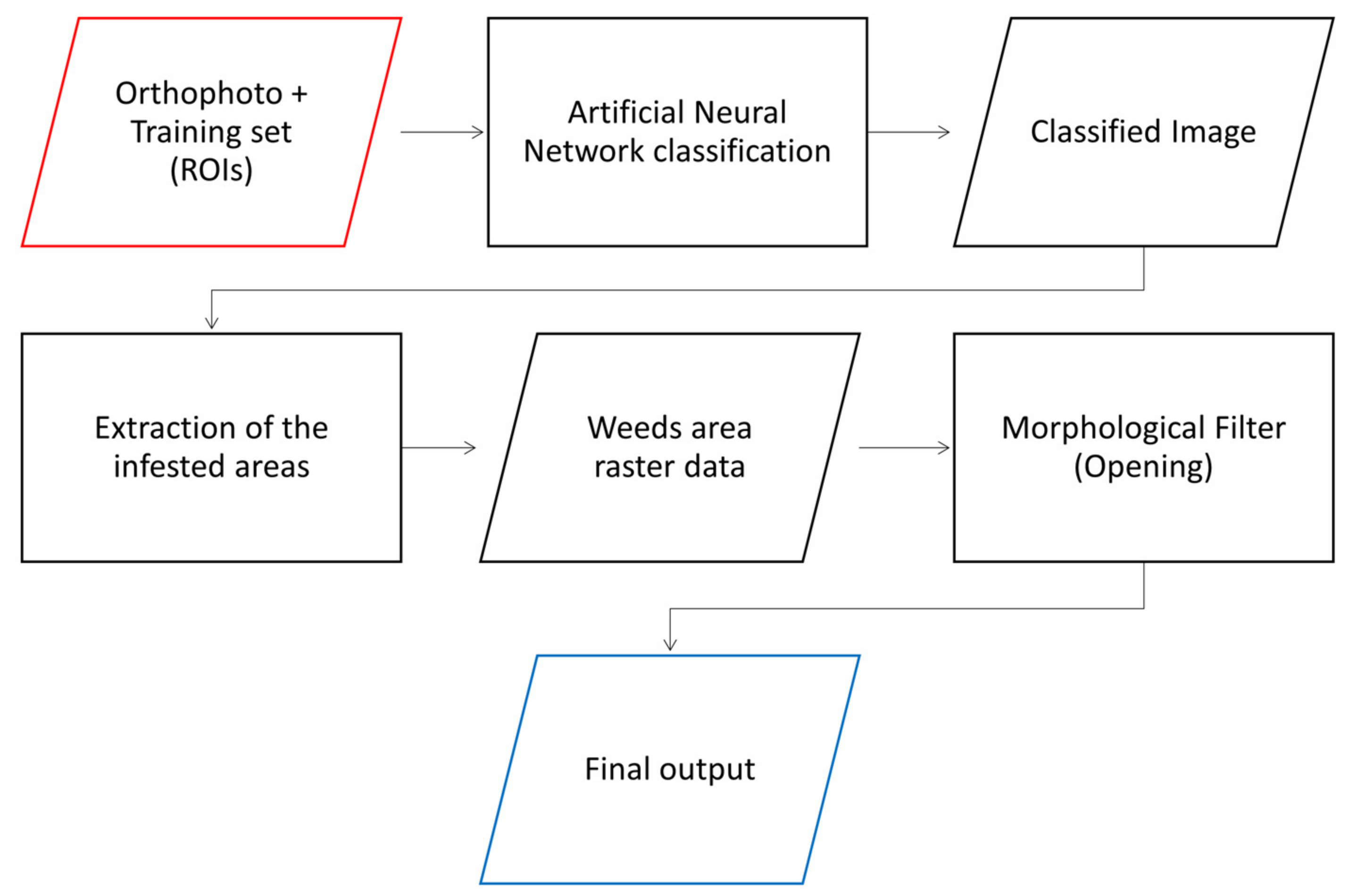
2.3.2. Artificial Neural Network (OpenCV)—ANN

The second method is based on Artificial Neural Network models of the OpenCV library implemented in the open-source software SAGA GIS. In fact, such a tool integrates in the GIS package the OpenCV Machine Learning library for Artificial Neural Network (ANN) classification of gridded features. The tool requires grid and vector data as inputs: the former is a three bands raster as an orthophoto processed from UAS survey (RGB bands in the range of visible spectrum), the latter samples areas which define ROIs for training regions. Then, it is necessary to set the parameters of the tool which determine the structure and functioning for the ANN model. These settings allow the user to define the number of hidden layers and their number of neurons, the number of iterations and the minimum variation of the error between iterations to make the algorithm stop, the parameters defining the activation function and those regarding the training method and learning rate. The outcome of the ANN model is a raster data expressing a value for each pixel which corresponds to the classes defined by the training dataset [55,56].
The ANN was trained with the same training set used in the Maximum Likelihood classification. As for MLC, downstream of the ANN classification, a morphological opening was performed to the weed class raster data in order to improve the spatial continuity as well as to eliminate spurious pixels in the outcome. After several attempts, the best output, based on visual interpretation, was achieved with the ANN parameters set as in Table 1. The final morphological opening was performed with an elliptical kernel with a size of 3 pixels. The workflow of the main processes and functions is summarized in Figure 3.

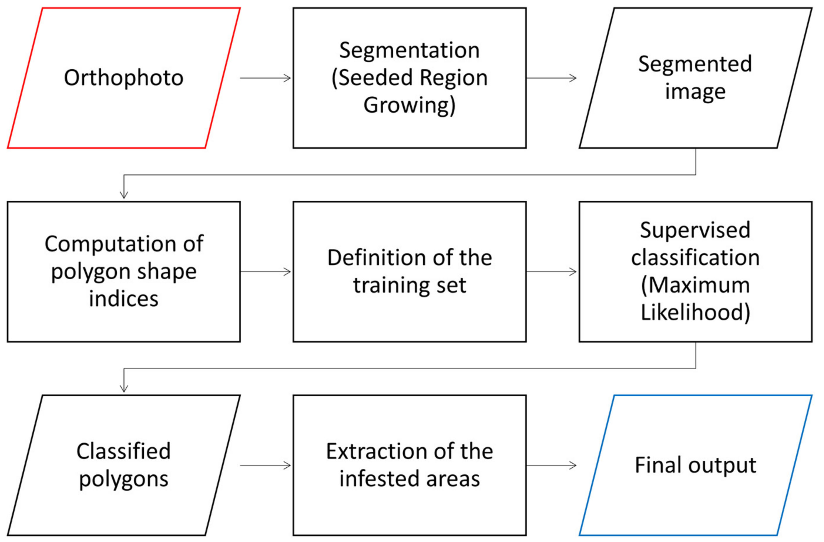
2.3.3. Object-Based Image Analysis—OBIA

Object-Based Image Analysis (OBIA) does not classify the image pixel-wise, and instead it is object oriented. This means that the classification is not performed for single pixels, but for groups of pixels. This approach is widely used in remote sensing image analysis, and also within the precision agriculture framework for applications such as weed and tree detection [19,44,57,58]. The groups of pixels are recognized as objects thanks to a pre-classification process called segmentation, which subdivides the image in different regions (objects) based on a certain homogeneity or similarity criterion. This weed detection method was adopted in our study by using the Object Based Image Segmentation, Polygon Shape Indices and Supervised Classification for Shapes tools of SAGA GIS. The first step, which is the image segmentation, uses a Seeded Region Growing algorithm. This algorithm is a segmentation technique which merges neighboring pixels, starting from a limited number of single pixels, called seeds, based on their spatial and spectral distances to the seed/cluster [57,59].
The output of this step is a polygonal vector file. The mean value of the pixels for every spectral band of all the polygons is computed and stored in its attribute table. The algorithm parameters were set in order to obtain a segmentation able to outline the infested area in the most accurate way. The correct definition of these parameters may require several runs of the model. The Band Width for Seed Point Generation parameter controls the distance, and thus the density, of the seed points. The Neighborhood parameter allows the user to choose between the von Neumann (4 connected pixels) and the Moore (8 connected pixels) neighborhood. The Variance in Feature Space and in Position Space parameters control the merging criteria and the relative influence of features and position space. The Generalization parameter specifies the search radius of a majority filter applied to smooth the result. More information on the algorithm and its parameters can be found in Bechtel et al. [57]. The final parameters settings for the Seeded Region Growing step are reported in Table 2.
Using the Polygon Shape Indices tool, it was possible to compute, for all the extracted polygons, some indices able to describe the polygons’ shape. These indices are mostly based on the area, the perimeter and the maximum diameter of the polygon [60,61].
Hence, the user needs to link some of the polygons to the specific classes to be identified: weed, crop and bare soil, in this case. This is performed by manually updating a column of the attribute table of the segmented file, which has been previously created, with the class identifier. These labelled polygons will work as training set for the classification tool: 70 polygons were labeled as weed, 150 as bare soil and 50 as maize. By checking the values of the shape indices for the polygons labelled as weed, maize or bare soil for the training set, it was possible to identify the most significant shape index. These indices were added as input for the polygon classification. The final classification was performed using the Supervised Classification for Shapes tool, which classified the polygons using the mean value of the Red, Green and Blue bands and the P/A shape index (i.e., the ratio between perimeter and area), using the polygons of the training set as a reference. The workflow of the main processes and functions is summarized in Figure 4.

2.3.4. Accuracy Assessment

Accuracy assessment of the tested methods was performed by adopting two approaches:
(i) The classification accuracy was assessed by means of an error matrix (or confusion matrix), which is a very common technique for the evaluation of classifications of remote sensing data. An error matrix consists in a square array, whose number of rows and columns correspond to the classes considered in the classification. In this case the classes are “non-weed” and “weed” (i.e., non-infested areas and infested areas). For every class, the number of pixels is reported in relation to the actual category recognized by the reference data. In this way it is possible to categorize the image pixels as: correctly classified as weed (true positive—TP), correctly classified as non-weed (true negative—TN), incorrectly classified as weed (false positive—FP) and incorrectly classified as non-weed (false negative—FN) [62]. In this study, the reference data is a map of the infested areas identified through visual interpretation of the orthomosaic and digitized. In this case, we are evaluating a binary classification with an unbalanced dataset; this means that the number of pixels in the weed class is much lower than the number of non-weed pixels. Consequently, the usual performance metrics computed from the confusion matrix, such as Overall Accuracy and F1 score, might be overoptimistic. For this reason, Chicco and Jurman [63] suggested the use of the Matthews Correlation Coefficient (MCC) for the evaluation of unbalanced binary classifications, rather than the most popular metrics. The MCC is a contingency matrix method for the Pearson product-moment correlation coefficient computation, between actual and predicted values. The MCC generates high scores only if the binary predictor is able to correctly predict the majority of positive cases and the majority of negative cases, independently of their ratios in the overall dataset. The value range of the MCC is (−1, +1), with extreme values −1, corresponding to perfect misclassification, and +1, corresponding to perfect classification. In such cases, i.e., unbalanced datasets, Overall Accuracy results in very high values providing overoptimistic estimation of the classifier performances. Compared to an F1 score, MCC performs better because it is invariant to class swapping and it depends also on the number of instances correctly classified as negative. This leads to a better estimation of the classifier performance in unbalanced datasets [63]. Therefore, we decided to include the MCC measure in our assessment. Starting from the error matrix, the Overall Accuracy (Equation (1)), the F1 score (Equation (2)) and the MCC (Equation (3)) were computed, as well as the commission and omission errors (Equations (4) and (5)) for the weed class, which are the complement values of the recall value (or Producer’s Accuracy) and of the precision value (or User’s Accuracy), respectively [62,63].
Overall   Accuracy = TP + TN TP + TN + FP + FN
F 1   score = 2 · TP 2 · TP + FP + FN
MCC = TP · TN FP · FN TP + FP · TP + FN · TN + FP · TN + FN
Commission   Error = 1 Precision = 1 TP TP + FP
Omission   Error = 1 Recall = 1 TP TP + FN
However, this first assessment uses a pixelwise approach, while the prescription maps are produced on the basis of the percentage of infested area per treatment cell. Hence, in order to understand the performances of the three methods from an operational point of view, and thus to better understand how these different accuracy values would affect the weed management, another assessment was performed.
(ii) This second assessment is based on the differences of infested area, since the percentage of infested area per treatment cell is a fundamental parameter for the prescription maps’ generation. For this purpose, the field was divided into 0.25 m2 square cells. For each cell, the percentage of infested area was computed according to the reference dataset and the three methods. Therefore, by computing the difference in the percentage of infested area for each cell, between the reference dataset and the MLC, the ANN and the OBIA methods, it was possible to compare the behavior of these methods from a more practical and concrete perspective. A negative value of this difference indicates an overestimation produced by the classification methods, while a positive value an underestimation.
It is important to point out that this accuracy assessment is based on the quality of photointerpretation. Therefore, the reference data are strongly influenced on one hand by the operator’s experience, ability, and precision, and on the other hand by the image quality. As a consequence, the accuracy values should be considered as indicative of the performances of these methodologies in weed mapping compared to human execution, and not as real accuracy measurements.

2.4. Prescription Map Creation

The main output product of a SSWM is the prescription map, which is the outcome of the process which allows the site-specific approach from an operational point of view. The prescription maps can be obtained by dividing the field with a grid and by computing, for every grid cell, the percentage of area covered by weed. Hence, a threshold is set, above which herbicide application is required [17].
In this case, the weed map obtained by the best detection method was used for the prescription map creation. This was performed by parceling out the field orthophoto in 0.25 m2 square cells. The percentage of infested area per cell was computed using the selected weed map. Consequently, all the cells showing a percentage of infested area higher than 10% were classified as cells needing treatment.

3. Results

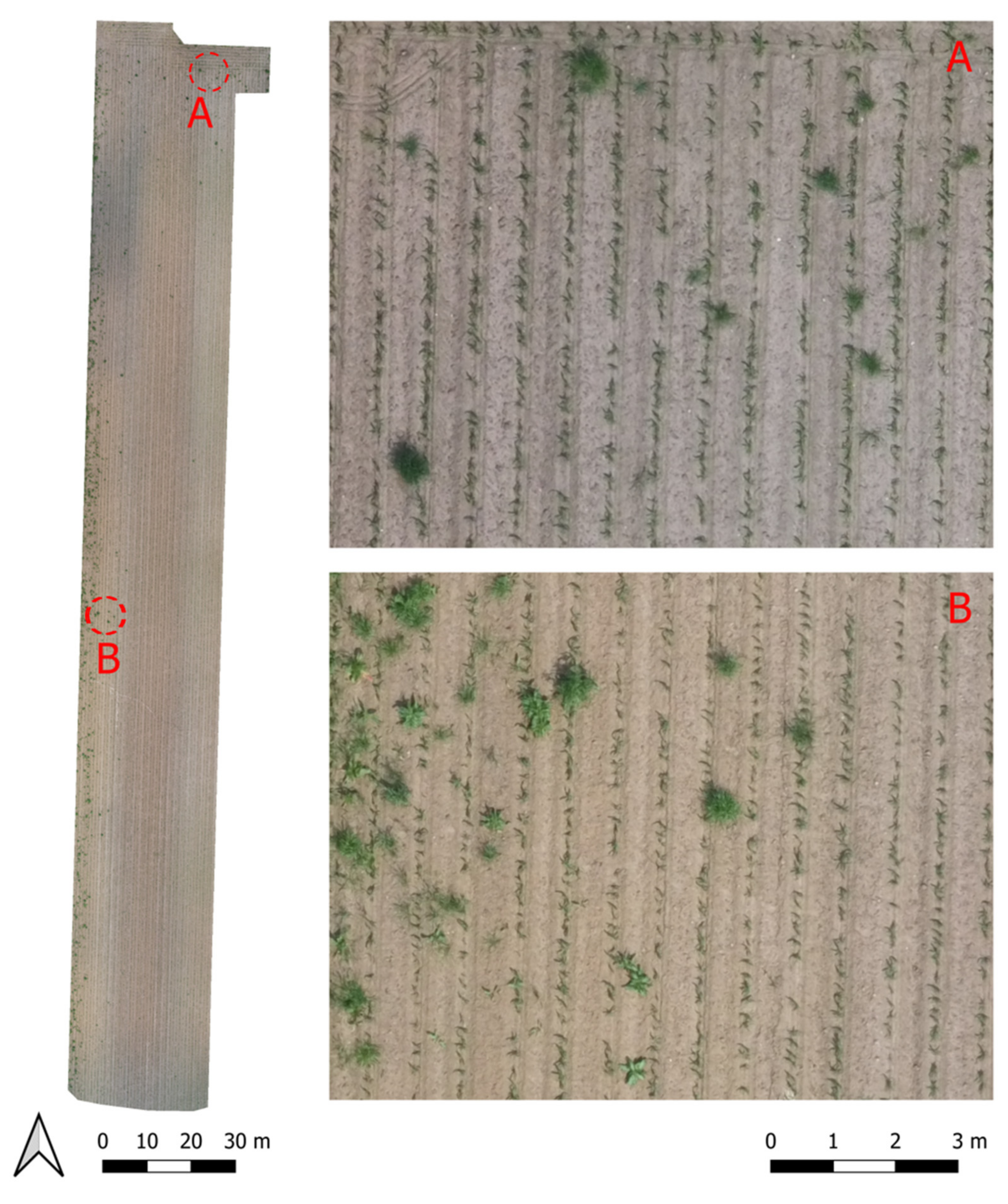
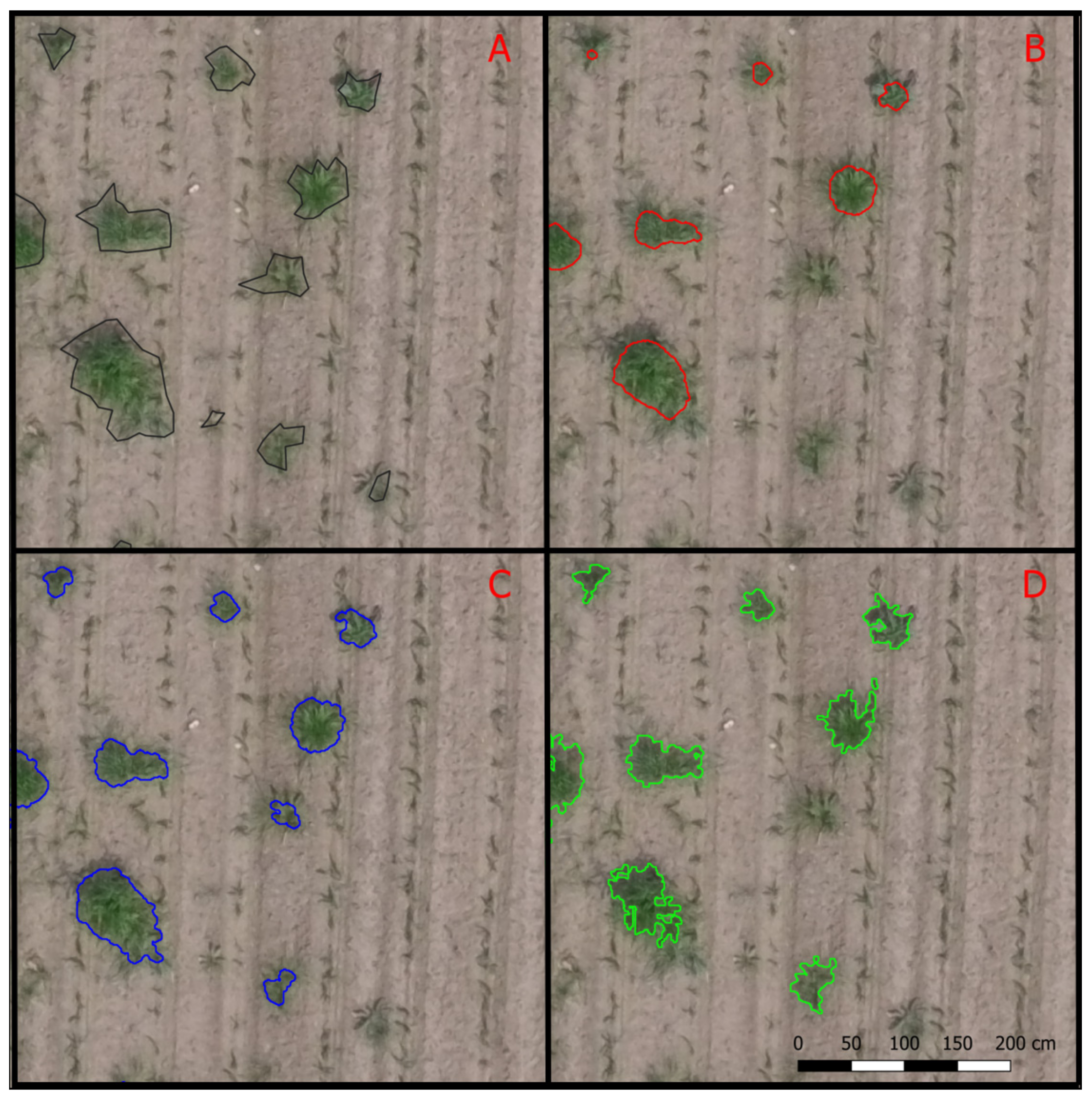
3.1. Very High Resolution Orthomosaic Generation and Weed Mapping by Photointerpretation

An orthorectified photomosaic at very high spatial resolution (1.09 cm/pixel) was generated by using Web ODM open-source software. The use of discrete points as control points allowed for the obtaining of a georeferenced orthophoto and the optimization of time and resources without adopting the conventional UAS targets and expensive technologies for precise topographic survey by GPS or RTK technologies.
Even if the presence of clouds produced heterogeneous lighting conditions, the detailed orthophoto allowed for easy identification and analyzing by visual interpretation the presence of weeds, both on rows and inter-rows (Figure 5). Mapping by photointerpretation at very high resolution allowed therefore the identification of 103.1 m2 of weed-infested areas, which represented 1.31% of the surveyed crop field. These areas were adopted as reference data for the accuracy assessment.

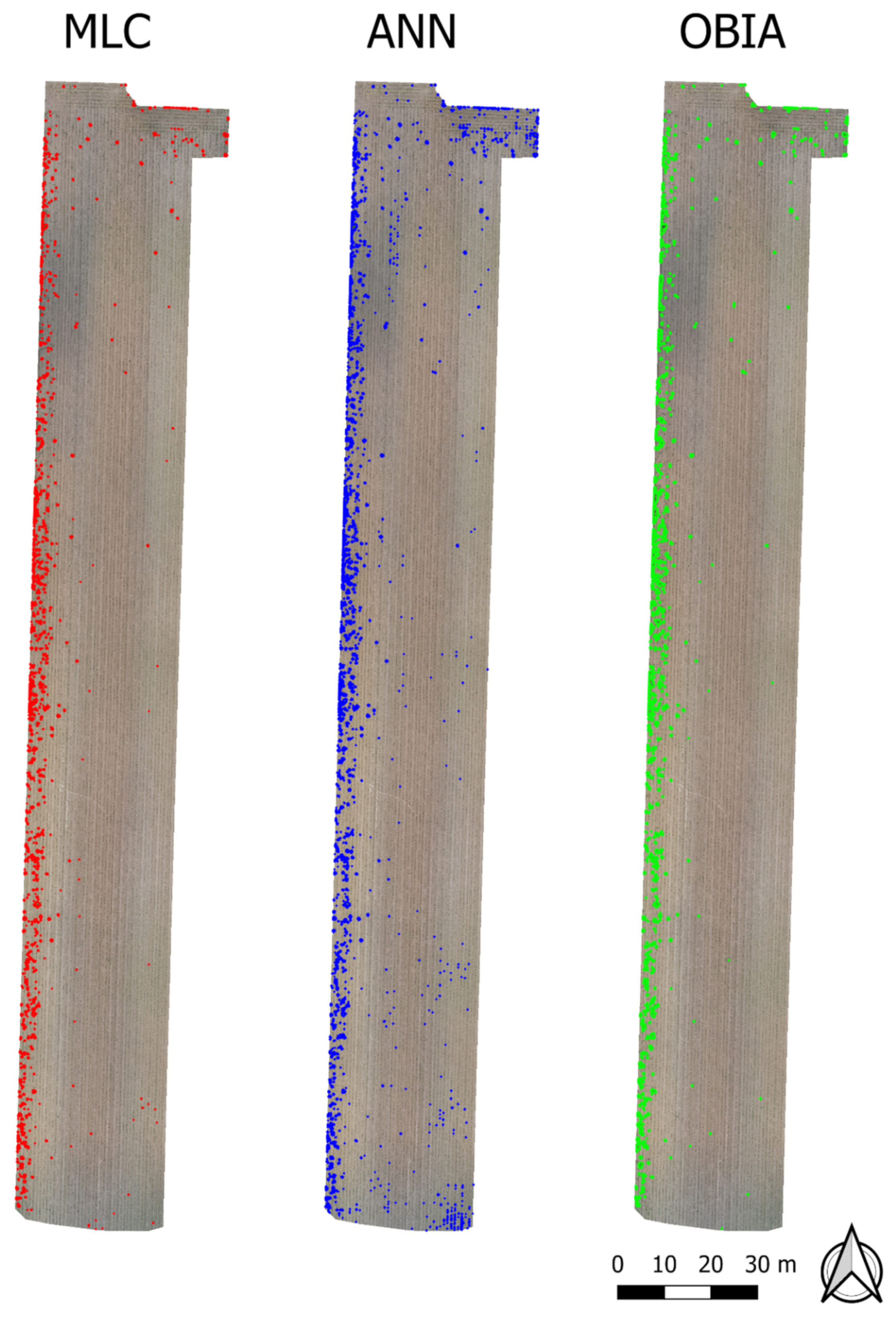
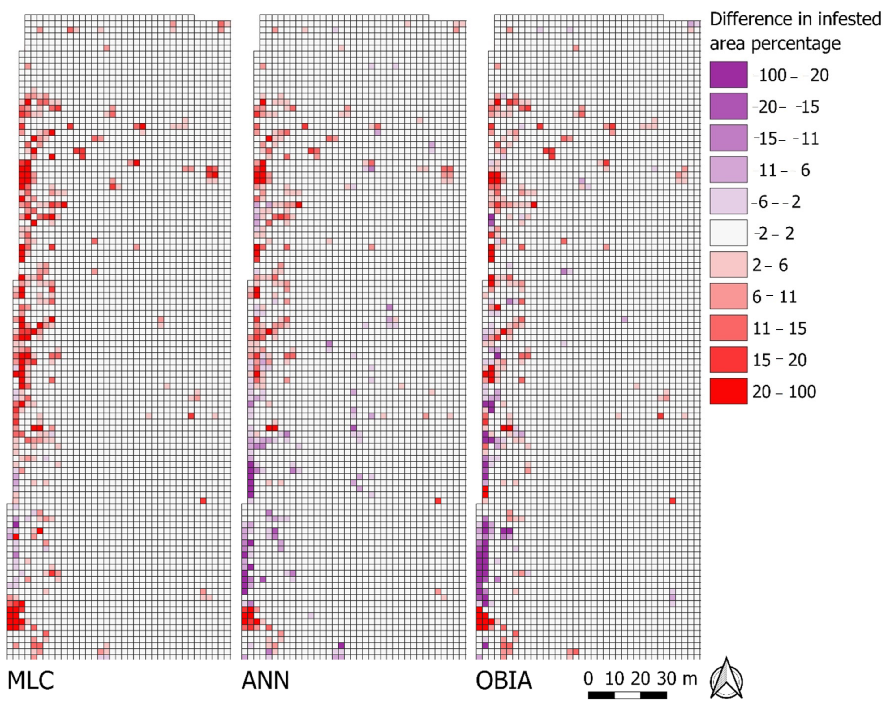
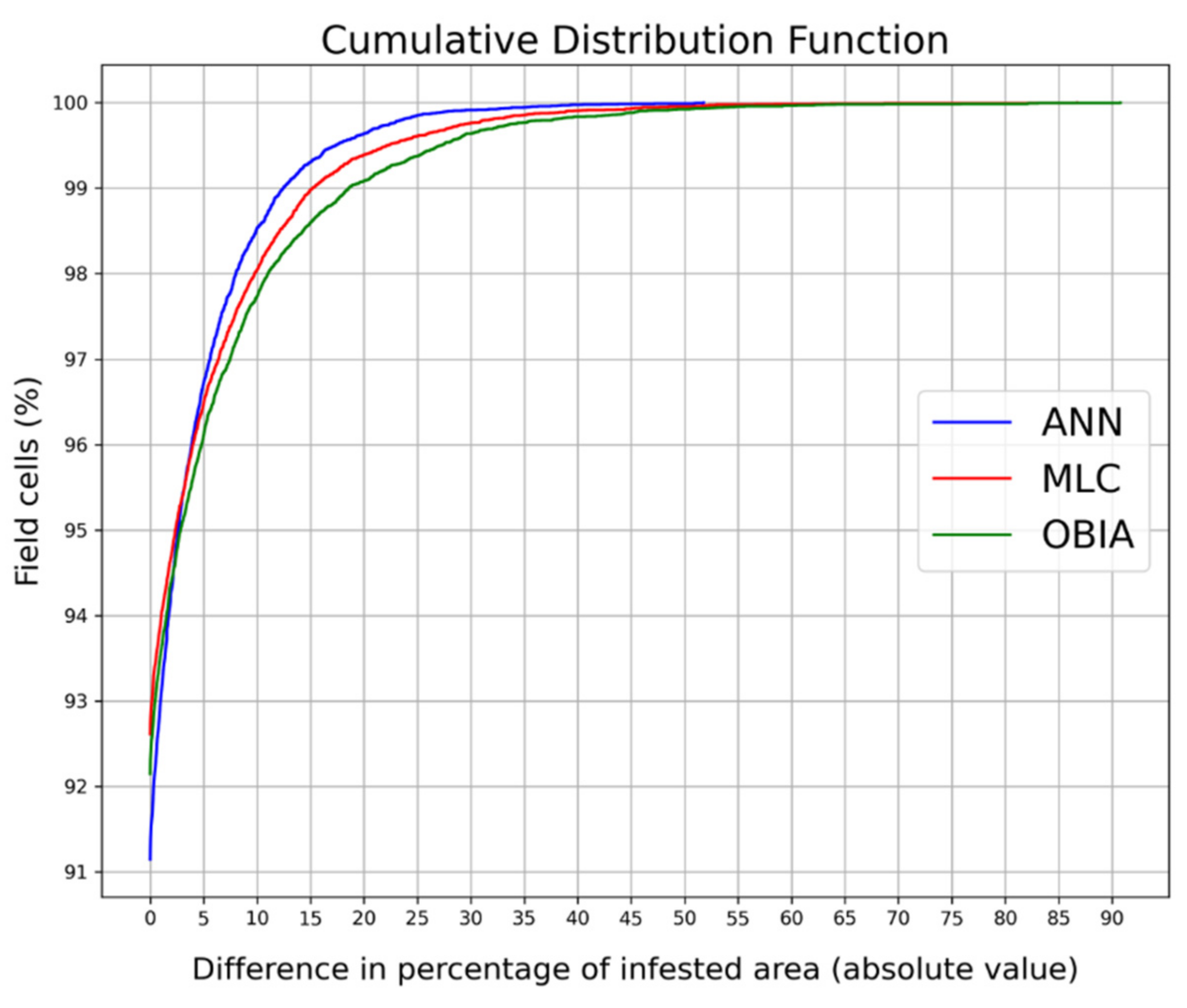
3.2. Semi-Automatic Weed Mapping and Prescription Map Creation

Semi-automatic extraction and classification allowed the mapping of 114.6 m2 for OBIA, 94.1 m2 for ANN, 69 m2 for MLC (Figure 6 and Figure 7).
The overall accuracy, computed through the error matrices, is very high for all the tested methods: 99.55% for the ANN method, 99.50% for the MLC method, and 99.38% for the OBIA method. Furthermore, this measure is strongly affected by the imbalance between the number of infested pixels and non-infested pixels. Therefore, it should not be considered as good descriptor of the algorithm’s performance. The F1 score suggests a good coherence between the tested methods and the reference dataset. The highest F1 score is 0.74 obtained from the ANN method, while the OBIA method produced an F1 score of 0.67 and the MLC method a value of 0.66. Additionally, the MCC values showed good performances of the tested weed detection methodologies. The highest MCC value is 0.74, obtained from the ANN method, followed by the MLC method with a MCC value of 0.68 and the OBIA method with a value of 0.67. The values of the omission and commission errors are more variable. The best trade-off is given by the ANN method, followed by the OBIA method, while the MLC method presents the lowest commission error but the highest omission error. A summary of the results is reported in Table 3. To facilitate the understanding of the MCC and its comparison with the other metrics, the normalized MCC (nMCC), which is simply the linear projection of the original range into the interval (0, 1), has also been reported in Table 3.
Regarding the differences in infested area per 0.25 m2 treatment cells, all three methods presented a good coherence with the reference dataset. In all cases, more than 91% of the field cells showed a difference in percentage of infested area equal to 0%. In particular, the difference in percentage of infested area, here considered in absolute value, is equal to 0% for the 92.5% of the cells in the MLC method, for the 91.1% of the cells in the ANN method and for the 92.1% of the cells in the OBIA method. However, the ANN method is the one with the fastest error decrease, with a value of the 99th percentile equal to a difference of 12.44% in the percentage of infested area in absolute value, compared to the 15.18% of the MLC method and the 18.58% of the OBIA method. For the MLC method, the 1.81% of the cells showed a negative difference, which means that the method identified a greater infested area in respect to the reference map, and the 5.63% of the cells showed a positive difference (i.e., the method identified a smaller infested area). For the ANN method, the 4.22% of the cells presented a negative difference, while the 4.67% a positive difference. For the OBIA method, the 3.79% of the cells showed a negative difference and the 4.10% a positive difference. Thus, regarding the number of cells needing treatment, ANN is the most overestimating method, while the MLC method is the most underestimating one. However, it is important to point out that this last statement considers only the number of cells deviating from the reference data, without quantifying this deviation. The maximum differences per cell found between the reference data and the tested methods are: 86.76% for the MLC method, 51.79% for the ANN method and 90.78% for the OBIA method (Figure 8 and Figure 9).
Regarding the first assessment based on confusion matrices, the ANN method clearly performed better than the other methodologies in all the proposed metrics. However, considering the evaluation based on the percentage of infested area, all the tested methods showed no differences with the reference data for more than the 90% of the cells. These results demonstrate that all the three tested methodologies showed good performances in weed detection, although with different accuracies. According to both the conducted assessments, the best result is undoubtedly obtained by adopting the ANN method. However, it is worth mentioning within the framework of this study, that even the simplest method, such as the MLC, turned out to be able to successfully detect the great majority of the field areas needing treatment.
Once the weed map is extracted it is possible to create a prescription map. This is done by parceling out the field in regular cells and by setting a threshold to the percentage of infested area per cell: in this way it is possible to plan a targeted weeding operation.
In this case study, the best results in weed detection were given by the ANN method, thus its output was chosen as input for the prescription map creation. For this purpose, the field was divided into 0.25 m2 square cells and the percentage of infested area was computed for each cell.
Finally, a prescription map was obtained by enacting a threshold equal to the 10% of infested area (i.e., all the cells with more than the 10% of infested area need treatment) (Figure 10). The resulting prescription map consists of 31,966 cells of which 1,108 identified as to be treated, equal to the 3.47% of the total cells.

4. Discussion

4.1. From UAS to Prescription Maps for Site-Specific Weed Management: Opportunities and Limitations

Adopting SSWM would bring to a drastic reduction of herbicide doses compared to conventional application methods that would comprise spraying the entire field. By the development of precision spray technology, prescription maps produced with weed recognition algorithms on orthophotos provided by the UAS could allow for performing herbicide treatment only where effectively needed, in locations where there is a weed presence beyond the decision threshold. This could bring a number of positive effects such as herbicide usage reduction, lesser cost of crop production and a healthier environment. Spraying only certain areas of the field could also be beneficial for the overall yield by reducing the risk of herbicides’ possible toxic effects on crop plants [64]. In addition, considering that the permitted amount of herbicides per hectare is trending to be reduced, spraying only the infested areas would limit herbicide use. In this way, some serious effects could be avoided or at least attenuated, such as herbicide resistance development, a phenomenon less likely to occur when lesser dosages are used [65]. Other than for herbicide use reduction, these prescription maps also have the potential to be used for optimization of different weed controlling methods such as the use of flames.
Our results showed that the combination of using a low-cost UAS to acquire very high-resolution imagery together with semi-automatic techniques is suitable to accurately map weed distribution in early-stage conventional maize field. The survey performed with a low-cost drone and open flight planning software, and the subsequent elaboration with OpenDroneMap, was able to produce a very high resolution orthomosaic (0.01 m/pixel), perfectly suitable for weed detection. The quality of the image allowed for easy recognition of weed, crop and soil. Thus, it made possible to delineate the ROIs required for the training of the classifiers and to produce the dataset used as reference for the accuracy assessment. The evaluation of the three weed detection methodologies highlighted the potential of modern classification techniques, such as ANN, the good performances of such methods and the good level of maturity reached by open-source packages. Specifically, the evaluation conducted by means of the confusion matrix shows that the tested methods performed well, above all the ANN method which is associated to high values of the proposed metrics, especially regarding the MCC (Overall Accuracy = 99.5%, F1-score = 0.74, MCC = 0.74, precision = 0.78 and recall = 0.71). In fact, our classification outputs are comparable, with the due distinctions, in terms of F1 score and Overall Accuracy to the results obtained in similar works: Peña et al. [19] mapped three different weed coverage categories in an early-season maize field, using an UAS with a six-band multispectral camera and an automatic OBIA procedure, with an Overall Accuracy equal to 86%; Gao et al. [66] applied a semi-automatic OBIA procedure combined with Random Forests and features selection techniques to classify soil, weed and maize in a post-emergence maize field, obtaining an Overall Accuracy of 94.5% (based on a 5-fold cross validation); Sivakumar et al. [44] tested two different deep learning models for mid- to late-season weed detection in a soybean field, obtaining precision, recall and F1 score values, for the best performing model, equal to 0.66, 0.68 and 0.67, respectively. It is important to highlight that in this specific case study, because of the imbalance in the dataset, the values of Overall Accuracy and F1 score might be overoptimistic. However, the high values of the MCC (MCC = 0.74 and nMCC = 0.87, for the ANN method), which is a better descriptor of the algorithm performance for this kind of dataset, confirm these good results. These considerations are not suited to compare weed detection methods, whose performances are strictly linked to the specific case study, but confirm that the degree of accuracy achieved is in line with that of similar research. Further confirmation of the good performances comes from the assessment based on the difference in infested area per cell, with all the proposed methods showing no differences to the reference dataset for more than the 90% of the cells and a deviation lower than 18% for 99% of the treatment cells. Most importantly, this study proves that the use of low-cost equipment together with open-source software can be used to successfully produce prescription maps: this opens up the possibility to adopt a SSWM strategy to a very wide audience, allowing drastic reduction in herbicide consumption, and thus of costs and environmental impacts.
Some technical limitations were nevertheless identified along the weed extraction process: firstly, since the crop was at early post-emergence stages, the maize plants were very small. Therefore, the pixels corresponding to crop were strongly contaminated by shadows and soil, even though the orthophoto resolution was very high. For this reason, many pixels corresponding to shadows or to transition areas between vegetation and bare soil were misclassified as crops. In addition, the heterogeneous lighting conditions of the field may lead to misclassification, in particular to commission errors for the weed class. Moreover, the dimensions of the training set proved to be highly relevant regarding the quality of the final output. Hence, in the case of poor classification results, increasing the training set dimension may be the fastest and the most effective way to improve the classification results.
In case of more complex scenarios, the best weed detection may be achieved combining more than one of the methods pointed out in this study: for example, an OBIA approach may be used to identify and mask crop rows first, and then a pixel-wise classification can be used to detect weeds, as done by Peña et al. [19], or by combining different image analysis techniques for the extraction of spatial information as in Louargant et al. [37]. The performances may increase also using as inputs other products obtainable trough such a drone survey like the DSM, in order to include also the plants height in the analysis [51]. Such approaches could improve the weed detection accuracy and help to automate the process.
Further improvements may be obtained using more advanced sensors, such as multi-spectral cameras. However, this involves additional expense both in terms of equipment and expertise.

4.2. Low-Cost UAS and GIS Open-Source: Towards a More Inclusive Smart Farming?

Despite the ecological and economic advantages that PAT can bring, the adoption of geospatial information technologies (i.e., satellite-based or UAS-based mapping), which are the basis of several smart farming practices, like SSWM, is critical [67]. The main concern for the farmers is given by the uncertainty of profitability, which is heightened by feasibility considerations and high investment costs. In fact, if larger farms may be more interested to adopt PATs, small-medium farms may be less involved: in fact, farm size is recognized as one of the main driving factors in PATs adoption. This is due to the fact that the farm size is related to the economic size of the farm, and thus to the capacity to absorb costs and risks [68,69,70]. As a consequence, the perception of usefulness of these tools becomes very important to by non-adopters of PATs: low-cost and easy-to-use devices tend to be considered more useful, even if they may be less accurate and with low performances. Therefore, to increase the spread of PATs, and thus of precision farming practices, the reduction of costs becomes a key factor, in order to address the needs of smaller farms and less high-tech oriented farmers [69,71].
These elements become even more crucial in developing countries, which show the biggest gap in PATs adoption for medium and small farms, especially if they do not use motorized mechanization. In some case, like China, small farms are actually characterized by an overuse of chemical inputs, compared to larger farms [72]. Therefore, as part of the strategies to spread the adoption of smart agriculture technologies in the developing world, it is very important to develop cost-effective tools and open-source geospatial technologies able to address the specific issues faced in such countries [67,73].
This is particularly relevant for UASs, which can be used also in organic or agro-ecological farming to scout and monitor fields in order to prevent yield losses from weeds, insects and diseases.

5. Conclusions

This study proposes a completely low-cost and open-source weed detection system and workflow. Beside the cost reduction, the use of open-source software (characterized by open licenses, source code repositories, manuals and tutorials) could speed up the development of free and specific tools for smart farming, and thus its adoption worldwide.
The open technology can contribute, behind the different declinations of precision/sustainable farming, toward the challenge of agroecological transition [74], beyond the first two levels of reduction and substitution.
In fact, weed management by reducing the use of herbicide is one of the challenges for increasing sustainability in conventional agriculture. Off-field impacts of herbicides may represent risks in terms of ecosystem degradation and human health. At present, an efficient alternative to chemical weed control is still lacking, pushing for the integration of new geospatial technologies in more sustainable agricultural practices. This work contributes to one of the possible solutions by combining a spatially explicit approach such as SSWM with the use of small low-cost UAS for very high resolution image processing. The main issue related to the scarce adoption of UAS in small-medium size farms is represented both by costs and the lack of knowledge and technology transfer. Therefore, cost reduction and knowledge sharing are the main issues that this sector has, at present, to face.
In this study a workflow for weed detection in an early-stage maize field has been proposed, using a low-cost UAS and only open-source software packages.
The results showed good performances of the tested technologies in all the process steps: UAS survey, orthomosaic generation, semi-automatic weed detection and prescription maps generation. The open-source photogrammetry software OpenDroneMap was successfully able to produce a very high-resolution orthomosaic (0.01 m/pixel) from the photos acquired by using a small and low-cost UAS. For the semi-automatic weed detection, three different methodologies were tested: all of them, even the simplest method, were able to successfully map most of the weeds present in the field. Finally, a prescription map for in situ management was generated, giving a practical agronomic scenario for weed management to drastically reduce herbicide doses.
Further studies should test these technologies on more complex scenarios, improving the use and development of open computer vision algorithms, which proved to be very appealing for these kinds of applications, as this study showed. Further improvements in weed detection may also be reached by adding other information, such as plant height. This data can be easily obtained from the DTM and DSM, which can be generated by using a low-cost UAS together with Open Drone Map.
Finally, this study shows the potential use of small low-cost UAS, together with open-source software and algorithms, for a widespread adoption of these geospatial technologies but also for a rapid development of open smart agriculture tools and software.

Author Contributions

Conceptualization, P.M. and S.E.P.; Methodology, P.M. and S.E.P.; Software, P.M., L.M.; Validation, P.M., S.E.P. and N.N.; Formal Analysis, P.M. and S.E.P.; Investigation, S.E.P., P.M., N.N. and A.P.; Resources, S.E.P., P.M., M.D.M., R.M. and A.P.; Data Curation, A.P., S.E.P. and P.M.; Writing-Original Draft, P.M., N.N. and S.E.P.; Writing-Review & Editing, P.M., S.E.P., M.D.M. and R.M.; Visualization, P.M., L.M. and S.E.P.; Supervision, R.M. and M.D.M.; Project Administration, P.M., S.E.P. and M.D.M. All authors have read and agreed to the published version of the manuscript.

Funding

This research was supported by the Master in GIScience and UAS (ICEA Department, University of Padua) (Italy).

Institutional Review Board Statement

Not applicable.

Informed Consent Statement

Not applicable.

Data Availability Statement

The datasets generated during the current study are available from the corresponding author on reasonable request.

Acknowledgments

We would thank the Master in GIScience and UAS (University of Padova) for the technical and logistic support; we also thank Bruno Casarotto for the UAS hardware support and the UAS survey.

Conflicts of Interest

The authors declare no conflict of interest.

References

  1. Lingenfelter, D.D.; Hartwig, N.L. Introduction to Weeds and Herbicides; Pennsylvania State University: College, PA, USA, 2013; pp. 1–38. [Google Scholar]
  2. Zimdahl, L.R. Fundamentals Of Weed Science, 3rd ed.; Elsevier: Amsterdam, The Netherlands, 2007; ISBN 9780080549859. [Google Scholar]
  3. Gharde, Y.; Singh, P.K.; Dubey, R.P.; Gupta, P.K. Assessment of yield and economic losses in agriculture due to weeds in India. Crop Prot. 2018, 107, 12–18. [Google Scholar] [CrossRef]
  4. Zimdahl, L.R. Introduction to Chemical Weed Control. In Fundamentals of Weed Science; Maragioglio, N., Fernandez, B.J., Eds.; Elsevier: Amsterdam, The Netherlands, 2018; pp. 391–416. ISBN 9780128111437. [Google Scholar]
  5. Arriaga, F.J.; Guzman, J.; Lowery, B. Conventional Agricultural Production Systems and Soil Functions. In Soil Health and Intensification of Agroecosytems; Elsevier: Amsterdam, The Netherlands, 2017; pp. 109–125. ISBN 9780128054017. [Google Scholar]
  6. Melander, B.; Rasmussen, I.A.; Bàrberi, P. Integrating physical and cultural methods of weed control— examples from European research. Weed Sci. 2005, 53, 369–381. [Google Scholar] [CrossRef]
  7. Astatkie, T.; Rifai, M.N.; Havard, P.; Adsett, J.; Lacko-Bartosova, M.; Otepka, P. Effectiveness of hot water, infrared and open flame thermal units for controlling weeds. Biol. Agric. Hortic. 2007, 25, 1–12. [Google Scholar] [CrossRef]
  8. Oerke, E.C. Crop losses to pests. J. Agric. Sci. 2006, 144, 31–43. [Google Scholar] [CrossRef]
  9. Kraehmer, H.; Laber, B.; Rosinger, C.; Schulz, A. Herbicides as Weed Control Agents: State of the Art: I. Weed Control Research and Safener Technology: The Path to Modern Agriculture. Plant Physiol. 2014, 166, 1119–1131. [Google Scholar] [CrossRef] [PubMed] [Green Version]
  10. Mohler, C.L. Ecological bases for the cultural control of annual weeds. J. Prod. Agric. 1996, 9, 468–474. [Google Scholar] [CrossRef]
  11. Weis, M.; Gutjahr, C.; Ayala, V.R.; Gerhards, R.; Ritter, C.; Schölderle, F. Precision farming for weed management: Techniques. Gesunde Pflanz. 2008, 60, 171–181. [Google Scholar] [CrossRef]
  12. Idowu, J.; Angadi, S. Understanding and Managing Soil Compaction in Agricultural Fields. Circular 2013, 672, 1–8. [Google Scholar]
  13. Sherwani, S.I.; Arif, I.A.; Khan, H.A. Modes of Action of Different Classes of Herbicides. In Herbicides, Physiology of Action, and Safety; Price, A., Kelton, J., Sarunaite, L., Eds.; InTech: London, UK, 2015; pp. 165–186. [Google Scholar]
  14. Gimsing, A.L.; Agert, J.; Baran, N.; Boivin, A.; Ferrari, F.; Gibson, R.; Hammond, L.; Hegler, F.; Jones, R.L.; König, W.; et al. Conducting Groundwater Monitoring Studies in Europe for Pesticide Active Substances and Their Metabolites in the context of Regulation (EC) 1107/2009. J. Consum. Prot. Food Saf. 2019, 14, 1–93. [Google Scholar] [CrossRef] [Green Version]
  15. Morales, M.A.M.; de Camargo, B.C.V.; Hoshina, M.M. Toxicity of Herbicides: Impact on Aquatic and Soil Biota and Human Health. In Herbicides: Current Research and Case Studies in Use; Price, A., Kelton, J., Eds.; IntechOpen Limited: London, UK, 2013; pp. 399–443. [Google Scholar]
  16. Liebman, M.; Baraibar, B.; Buckley, Y.; Childs, D.; Christensen, S.; Cousens, R.; Eizenberg, H.; Heijting, S.; Loddo, D.; Merotto, A.; et al. Ecologically sustainable weed management: How do we get from proof-of-concept to adoption? Ecol. Appl. 2016, 26, 1352–1369. [Google Scholar] [CrossRef]
  17. López-Granados, F.; Torres-Sánchez, J.; Serrano-Pérez, A.; de Castro, A.I.; Mesas-Carrascosa, F.J.; Peña, J.M. Early season weed mapping in sunflower using UAV technology: Variability of herbicide treatment maps against weed thresholds. Precis. Agric. 2016, 17, 183–199. [Google Scholar] [CrossRef]
  18. Castaldi, F.; Pelosi, F.; Pascucci, S.; Casa, R. Assessing the potential of images from unmanned aerial vehicles (UAV) to support herbicide patch spraying in maize. Precis. Agric. 2017, 18, 76–94. [Google Scholar] [CrossRef]
  19. Peña, J.M.; Torres-Sánchez, J.; de Castro, A.I.; Kelly, M.; López-Granados, F. Weed Mapping in Early-Season Maize Fields Using Object-Based Analysis of Unmanned Aerial Vehicle (UAV) Images. PLoS ONE 2013, 8, e77151. [Google Scholar]
  20. Barros, J.C.; Calado, J.G.; Basch, G.; Carvalho, M.J. Effect of different doses of post-emergence-applied iodosulfuron on weed control and grain yield of malt barley (Hordeum distichum L.), under Mediterranean conditions. J. Plant Prot. Res. 2016, 56, 15–20. [Google Scholar] [CrossRef]
  21. Swanton, C.J.; Shrestha, A.; Chandler, K.; Deen, W. An Economic Assessment of Weed Control Strategies in No-Till Glyphosate-Resistant Soybean (Glycine max). Weed Technol. 2000, 14, 755–763. [Google Scholar] [CrossRef]
  22. Sartorato, I.; Berti, A.; Zanin, G. Estimation of economic thresholds for weed control in soybean (Glycine max (L.) Merr.). Crop Prot. 1996, 15, 63–68. [Google Scholar] [CrossRef]
  23. Power, E.F.; Kelly, D.L.; Stout, J.C. The impacts of traditional and novel herbicide application methods on target plants, non-target plants and production in intensive grasslands. Weed Res. 2013, 53, 131–139. [Google Scholar] [CrossRef]
  24. Weis, M.; Keller, M.; Rueda, V. Herbicide Reduction Methods. In Herbicides-Environmental Impact Studies and Management Approaches; InTech: Rijeka, Croatia, 2012. [Google Scholar]
  25. European Parliament Directive 2009/128/EC of the European Parliament and the Council of 21 October 2009 establishing a framework for Community action to achieve the sustainable use of pesticides. Off. J. Eur. Union 2009, 309, 71–86.
  26. European Parliament. Precision Agriculture and the Future of Farming in Europe; European Parliamentary Research Service: Bruxelles, Belgium, 2016; ISBN 9789284604753.
  27. Kritikos, M. Precision Agriculture in Europe: Legal, Social and Ethical Considerations; European Parliamentary Research Service: Bruxelles, Belgium, 2017; ISBN 9789282368855. [Google Scholar]
  28. Andújar, D.; Barroso, J.; Fernández-Quintanilla, C.; Dorado, J. Spatial and temporal dynamics of Sorghum halepense patches in maize crops. Weed Res. 2012, 52, 411–420. [Google Scholar] [CrossRef]
  29. Lambert, J.P.T.; Hicks, H.L.; Childs, D.Z.; Freckleton, R.P. Evaluating the potential of Unmanned Aerial Systems for mapping weeds at field scales: A case study with Alopecurus myosuroides. Weed Res. 2018, 58, 35–45. [Google Scholar] [CrossRef] [Green Version]
  30. Huang, H.; Deng, J.; Lan, Y.; Yang, A.; Deng, X.; Wen, S.; Zhang, H.; Zhang, Y. Accurate weed mapping and prescription map generation based on fully convolutional networks using UAV imagery. Sensors 2018, 18, 3299. [Google Scholar] [CrossRef] [Green Version]
  31. Hanzlik, K.; Gerowitt, B. Methods to conduct and analyse weed surveys in arable farming: A review. Agron. Sustain. Dev. 2016, 36, 1–18. [Google Scholar] [CrossRef] [Green Version]
  32. Tamouridou, A.A.; Alexandridis, T.K.; Pantazi, X.E.; Lagopodi, A.L.; Kashefi, J.; Moshou, D. Evaluation of UAV imagery for mapping Silybum marianum weed patches. Int. J. Remote Sens. 2017, 38, 2246–2259. [Google Scholar] [CrossRef]
  33. Kim, D.-W.; Kim, Y.; Kim, K.-H.; Kim, H.-J.; Chung, Y.S. Case Study: Cost-effective Weed Patch Detection by Multi-Spectral Camera Mounted on Unmanned Aerial Vehicle in the Buckwheat Field. Korean J. Crop Sci. 2019, 64, 159–164. [Google Scholar]
  34. Dian Bah, M.; Hafiane, A.; Canals, R. Deep learning with unsupervised data labeling for weed detection in line crops in UAV images. Remote Sens. 2018, 10, 1690. [Google Scholar]
  35. Lin, F.; Zhang, D.; Huang, Y.; Wang, X.; Chen, X. Detection of corn and weed species by the combination of spectral, shape and textural features. Sustainability 2017, 9, 1335. [Google Scholar] [CrossRef] [Green Version]
  36. Maes, W.H.; Steppe, K. Perspectives for Remote Sensing with Unmanned Aerial Vehicles in Precision Agriculture. Trends Plant Sci. 2019, 24, 152–164. [Google Scholar] [CrossRef] [PubMed]
  37. Louargant, M.; Jones, G.; Faroux, R.; Paoli, J.N.; Maillot, T.; Gée, C.; Villette, S. Unsupervised classification algorithm for early weed detection in row-crops by combining spatial and spectral information. Remote Sens. 2018, 10, 761. [Google Scholar] [CrossRef] [Green Version]
  38. Fernández-Quintanilla, C.; Peña, J.M.; Andújar, D.; Dorado, J.; Ribeiro, A.; López-Granados, F. Is the current state of the art of weed monitoring suitable for site-specific weed management in arable crops? Weed Res. 2018, 58, 259–272. [Google Scholar] [CrossRef]
  39. Hunt, E.R.; Daughtry, C.S.T. What good are unmanned aircraft systems for agricultural remote sensing and precision agriculture? Int. J. Remote Sens. 2017, 39, 5345–5376. [Google Scholar] [CrossRef] [Green Version]
  40. Bakhshipour, A.; Jafari, A. Evaluation of support vector machine and artificial neural networks in weed detection using shape features. Comput. Electron. Agric. 2018, 145, 153–160. [Google Scholar] [CrossRef]
  41. Eddy, P.R.; Smith, A.M.; Hill, B.D.; Peddle, D.R.; Coburn, C.A.; Blackshaw, R.E. Comparison of neural network and maximum likelihood high resolution image classification for weed detection in crops: Applications in precision agriculture. Int. Geosci. Remote Sens. Symp. 2006, 116–119. [Google Scholar]
  42. Dos Santos Ferreira, A.; Matte Freitas, D.; Gonçalves da Silva, G.; Pistori, H.; Theophilo Folhes, M. Weed detection in soybean crops using ConvNets. Comput. Electron. Agric. 2017, 143, 314–324. [Google Scholar] [CrossRef]
  43. Thorp, K.R.; Tian, L.F. A review on remote sensing of weeds in agriculture. Precis. Agric. 2004, 5, 477–508. [Google Scholar] [CrossRef]
  44. Sivakumar, A.N.V.; Li, J.; Scott, S.; Psota, E.; Jhala, A.J.; Luck, J.D.; Shi, Y. Comparison of object detection and patch-based classification deep learning models on mid-to late-season weed detection in UAV imagery. Remote Sens. 2020, 12, 2136. [Google Scholar] [CrossRef]
  45. Wendel, A.; Underwood, J. Self-supervised weed detection in vegetable crops using ground based hyperspectral imaging. Proc. IEEE Int. Conf. Robot. Autom. 2016, 2016, 5128–5135. [Google Scholar]
  46. Zheng, Y.; Zhu, Q.; Huang, M.; Guo, Y.; Qin, J. Maize and weed classification using color indices with support vector data description in outdoor fields. Comput. Electron. Agric. 2017, 141, 215–222. [Google Scholar] [CrossRef]
  47. Toffanin, P. OpenDroneMap: The Missing Guide. A Practical Guide to Drone Mapping Using Free and Open Source Software; MasseranoLabs LLC.: Saint Petersburg, FL, USA, 2019; ISBN 978-1086027563. [Google Scholar]
  48. Conrad, O.; Bechtel, B.; Bock, M.; Dietrich, H.; Fischer, E.; Gerlitz, L.; Wehberg, J.; Wichmann, V.; Böhner, J. System for Automated Geoscientific Analyses (SAGA) v. 2.1. Geosci. Model Dev. 2015, 8, 1991–2007. [Google Scholar] [CrossRef] [Green Version]
  49. Bolstad, P.V.; Lillesand, T.M. Rapid maximum likelihood classification. Photogramm. Eng. Remote Sens. 1991, 57, 67–74. [Google Scholar]
  50. Otukei, J.R.; Blaschke, T. Land cover change assessment using decision trees, support vector machines and maximum likelihood classification algorithms. Int. J. Appl. Earth Obs. Geoinf. 2010, 12, 27–31. [Google Scholar] [CrossRef]
  51. De Castro, A.I.; Jurado-Expósito, M.; Peña-Barragán, J.M.; López-Granados, F. Airborne multi-spectral imagery for mapping cruciferous weeds in cereal and legume crops. Precis. Agric. 2012, 13, 302–321. [Google Scholar] [CrossRef] [Green Version]
  52. Weiss, G.; Provost, F. The Effect of Class Distribution on Classifier Learning: An Empirical Study; Tech. Rep. ML-TR-44 Dep.; Computer Science Rutgers University: New Brunswick, NJ, USA, 2001; pp. 1–26. [Google Scholar] [CrossRef]
  53. Ustuner, M.; Sanli, F.B.; Abdikan, S. Balanced vs imbalanced training data: Classifying rapideye data with support vector machines. Int. Arch. Photogramm. Remote Sens. Spat. Inf. Sci. ISPRS Arch. 2016, 41, 379–384. [Google Scholar] [CrossRef]
  54. Said, K.A.M.; Jambek, A.B.; Sulaiman, N. A study of image processing using morphological opening and closing processes. Int. J. Control Theory Appl. 2016, 9, 15–21. [Google Scholar]
  55. Egmont-Petersen, M.; De Ridder, D.; Handels, H. Image processing with neural networks- A review. Pattern Recognit. 2002, 35, 2279–2301. [Google Scholar] [CrossRef]
  56. OPEN CV Neural Networks. Available online: https://docs.opencv.org/2.4/modules/ml/doc/neural_networks.html (accessed on 10 May 2021).
  57. Bechtel, B.; Ringeler, A.; Böhner, J. Segmentation for Object Extraction of Treed Using MATLAB and SAGA. Hamburg. Beiträge Phys. Geogr. Landsch. 2008, 19, 1–12. [Google Scholar]
  58. Ozdarici-Ok, A. Automatic detection and delineation of citrus trees from VHR satellite imagery. Int. J. Remote Sens. 2015, 36, 4275–4296. [Google Scholar] [CrossRef]
  59. Adams, R.; Bischof, L. Seeded Region Growing. IEEE Trans. Pattern Anal. Mach. Intell. 1994, 16, 641–647. [Google Scholar] [CrossRef] [Green Version]
  60. Forman, R.T.T.; Godron, M. Landscape Ecology; Wiley & Sons: Hoboken, NJ, USA, 1986. [Google Scholar]
  61. Lang, S.; Blaschke, T. Landschaftsanalyse Mit GIS; Eugen-Ulmer-Verlag: Stuttgart, Germany, 2007; ISBN 9783825283476. [Google Scholar]
  62. Congalton, R.G. A review of assessing the accuracy of classifications of remotely sensed data. Remote Sens. Environ. 1991, 37, 35–46. [Google Scholar] [CrossRef]
  63. Chicco, D.; Jurman, G. The advantages of the Matthews correlation coefficient (MCC) over F1 score and accuracy in binary classification evaluation. BMC Genom. 2020, 21, 1–14. [Google Scholar] [CrossRef] [Green Version]
  64. Boutin, C.; Strandberg, B.; Carpenter, D.; Mathiassen, S.K.; Thomas, P.J. Herbicide impact on non-target plant reproduction: What are the toxicological and ecological implications? Environ. Pollut. 2014, 185, 295–306. [Google Scholar] [CrossRef] [Green Version]
  65. Norsworthy, J.K.; Ward, S.M.; Shaw, D.R.; Llewellyn, R.S.; Nichols, R.L.; Webster, T.M.; Bradley, K.W.; Frisvold, G.; Powles, S.B.; Burgos, N.R.; et al. Reducing the Risks of Herbicide Resistance: Best Management Practices and Recommendations. Weed Sci. 2012, 60, 31–62. [Google Scholar] [CrossRef] [Green Version]
  66. Gao, J.; Liao, W.; Nuyttens, D.; Lootens, P.; Vangeyte, J.; Pižurica, A.; He, Y.; Pieters, J.G. Fusion of pixel and object-based features for weed mapping using unmanned aerial vehicle imagery. Int. J. Appl. Earth Obs. Geoinf. 2018, 67, 43–53. [Google Scholar] [CrossRef]
  67. Lowenberg-Deboer, J.; Erickson, B. Setting the record straight on precision agriculture adoption. Agron. J. 2019, 111, 1552–1569. [Google Scholar] [CrossRef] [Green Version]
  68. Tey, Y.S.; Brindal, M. Factors influencing the adoption of precision agricultural technologies: A review for policy implications. Precis. Agric. 2012, 13, 713–730. [Google Scholar] [CrossRef]
  69. Paustian, M.; Theuvsen, L. Adoption of precision agriculture technologies by German crop farmers. Precis. Agric. 2017, 18, 701–716. [Google Scholar] [CrossRef]
  70. Barnes, A.P.; Soto, I.; Eory, V.; Beck, B.; Balafoutis, A.; Sánchez, B.; Vangeyte, J.; Fountas, S.; van der Wal, T.; Gómez-Barbero, M. Exploring the adoption of precision agricultural technologies: A cross regional study of EU farmers. Land Use Policy 2019, 80, 163–174. [Google Scholar] [CrossRef]
  71. Pierpaoli, E.; Carli, G.; Pignatti, E.; Canavari, M. Drivers of Precision Agriculture Technologies Adoption: A Literature Review. Procedia Technol. 2013, 8, 61–69. [Google Scholar] [CrossRef] [Green Version]
  72. Wu, Y.; Xi, X.; Tang, X.; Luo, D.; Gu, B.; Lam, S.K.; Vitousek, P.M.; Chen, D. Policy distortions, farm size, and the overuse of agricultural chemicals in China. Proc. Natl. Acad. Sci. USA 2018, 115, 7010–7015. [Google Scholar] [CrossRef] [Green Version]
  73. Mondal, P.; Basu, M. Adoption of precision agriculture technologies in India and in some developing countries: Scope, present status and strategies. Prog. Nat. Sci. 2009, 19, 659–666. [Google Scholar] [CrossRef]
  74. Gliessman, S. Transforming food systems with agroecology. Agroecol. Sustain. Food Syst. 2016, 40, 187–189. [Google Scholar] [CrossRef]
Figure 1. (A) Veneto Region: Digital Elevation Model and localization of the study site; (B) study site at the Experimental farm “L. Toniolo” (University of Padova, NE Italy).
Remotesensing 13 01869 g001
Figure 2. Workflow for Maximum Likelihood classification weed mapping method.
Remotesensing 13 01869 g002
Figure 3. Workflow of the Artificial Neural Network weed mapping method: the only difference with the workflow shown in Figure 2 is in the first process, i.e., the classification algorithm.
Remotesensing 13 01869 g003
Figure 4. Workflow for the Object-Based Image Analysis weed mapping method.
Remotesensing 13 01869 g004
Figure 5. Study site: high resolution orthophoto at 1 cm pixel cell size derived from UAS survey, crop field surveyed (left) and details (right).
Remotesensing 13 01869 g005
Figure 6. Weed maps obtained with the MLC method, ANN method and OBIA method.
Remotesensing 13 01869 g006
Figure 7. Detail of the weed maps obtained with: (A) photointerpretation (reference data), (B) the MLC method, (C) ANN method, (D) and OBIA method.
Remotesensing 13 01869 g007
Figure 8. Comparison of the differences in weed area percentage per treatment cell for the three methods (detail).
Remotesensing 13 01869 g008
Figure 9. Cumulative distribution of the field treatment cells vs. the difference in percentage of infested area in absolute value.
Remotesensing 13 01869 g009
Figure 10. Detail of the northernmost part of the prescription map obtained by the ANN method with a threshold on the percentage of infested area per cell equal to 10%.
Remotesensing 13 01869 g010
Table 1. Artificial Neural Network parameters settings.
Number of Layers3
Number of Neurons12
Maximum Number of Iterations3000
Error change (Epsilon)0.0000001192
Activation FunctionSigmoid
Function’s Alpha1
Function’s Beta1
Training MethodBack propagation
Weight Gradient term0.1
Moment term0.1
Table 2. Object Based Image Segmentation parameters settings.
Band Width for Seed Point Generation22
Neighborhood8 (Moore)
DistanceFeature space and position
Variance in Feature Space3
Variance in Position Space10
Generalization2
Table 3. Accuracy assessment results summary for the three tested weed detection methods.
Overall
Accuracy %
F1 Score
(Range (0, 1))
MCC
(Range(−1, 1))
nMCC
(Range (0, 1))
Omission Error %Commission Error %
MLC99.500.66250.68170.840846.8911.95
ANN99.550.74520.74370.871828.7421.89
OBIA99.380.67790.67570.837828.4435.58
Publisher’s Note: MDPI stays neutral with regard to jurisdictional claims in published maps and institutional affiliations.

