Article

Measuring Alpha and Beta Diversity by Field and Remote-Sensing Data: A Challenge for Coastal Dunes Biodiversity Monitoring

by
Flavio Marzialetti
1,*,
Silvia Cascone
2,
Ludovico Frate
1,
Mirko Di Febbraro
1,
Alicia Teresa Rosario Acosta
2 and
Maria Laura Carranza
1
1
Envix-Lab, Departement of Biosciences and Territory, Molise University, Contrada Fonte Lappone, 86090 Pesche, Italy
2
Department of Sciences, Roma Tre University, Viale G. Marconi 446, 00146 Rome, Italy
*
Author to whom correspondence should be addressed.
Remote Sens. 2021, 13(10), 1928; https://doi.org/10.3390/rs13101928
Submission received: 31 March 2021 / Revised: 9 May 2021 / Accepted: 13 May 2021 / Published: 15 May 2021
(This article belongs to the Special Issue Remote Sensing of Ecosystem Diversity)

Abstract

:
Combining field collected and remotely sensed (RS) data represents one of the most promising approaches for an extensive and up-to-date ecosystem assessment. We investigated the potential of the so called spectral variability hypothesis (SVH) in linking field-collected and remote-sensed data in Mediterranean coastal dunes and explored if spectral diversity provides reliable information to monitor floristic diversity, as well as the consistency of such information in altered ecosystems due to plant invasions. We analyzed alpha diversity and beta diversity, integrating floristic field and Remote-Sensing PlanetScope data in the Tyrrhenian coast (Central Italy). We explored the relationship among alpha field diversity (species richness, Shannon index, inverse Simpson index) and spectral variability (distance from the spectral centroid index) through linear regressions. For beta diversity, we implemented a distance decay model (DDM) relating field pairwise (Jaccard similarities index, Bray–Curtis similarities index) and spectral pairwise (Euclidean distance) measures. We observed a positive relationship between alpha diversity and spectral heterogeneity with richness reporting the higher R score. As for DDM, we found a significant relationship between Bray–Curtis floristic similarity and Euclidean spectral distance. We provided a first assessment of the relationship between floristic and spectral RS diversity in Mediterranean coastal dune habitats (i.e., natural or invaded). SVH provided evidence about the potential of RS for estimating diversity in complex and dynamic landscapes.

Graphical Abstract

1. Introduction

Biodiversity loss due to human activities is accelerating at an extraordinary pace, and several researchers hypothesize that life on Earth is undergoing a mass extinction phenomenon [1], which makes continuous ecosystem monitoring a pressing need [2]. Nonetheless, regular assessment of biodiversity is difficult to undertake via field surveys [3].
The economic limitations in many countries restrict the possibilities of implementing monitoring programs based on large-scale fieldwork [4]. Furthermore, collecting extensive and representative data in the field could be hampered by the impossibility to reach some monitoring areas [5]. Systematically surveying and monitoring complex and dynamic ecosystems (e.g., coastal dunes or river banks) by conventional biodiversity field campaigns might not be possible due to high costs, challenges to access to some sampling sites and lack of historical data [6,7]. Such crucial limitations hamper implementing statistically sound monitoring schemes that are essential for better understanding and modelling biodiversity in space and time [8].
In contrast to field-based methods, satellite remote sensing (RS) providing frequent and complete spatial coverage is a cost-effective (free remotely sensed products) and comprehensive support for monitoring several biodiversity features at multiple spatial scales [9,10,11]. Furthermore, combining remotely sensed and in situ field data represents one of the most promising approaches to fill the gaps in biodiversity monitoring [4].
In 2002, Palmer and coauthors postulated the spectral variability hypothesis (hereafter SVH), stating that the larger the spectral heterogeneity of an environment the higher its biodiversity [3]. Since then, several research efforts have been devoted to explore the relationship between remotely sensed and field-collected data [12,13] accounting for both alpha diversity (e.g., within sample/pixel variability) [14] and beta diversity (e.g., between samples/pixels variability) [15]. The potential of SVH to depict alpha diversity was tested on several ecosystems covering large areas as evergreen forests [10], tropical forests [16], wetlands [17], grasslands [18], savannah woodlands [19]. Similarly, SVH was tested to explore beta diversity on Mediterranean shrubs and forests [15,20], tropical forests [21,22], deciduous forests [23] and grasslands [24]. However, little attention has been paid to extend SVH applications to more complex and dynamic landscapes [25]. In particular, the SVH effectiveness in depicting field and spectral diversity patterns on very dynamic ecosystems such as coastal dunes is still missing.
Coastal dunes environments occur on narrow strips of land interposed between marine and terrestrial realms [26,27]. The strong influence of continuous sudden changes on abiotic and biotic factors promotes the development of highly specialized biodiversity and a peculiar vegetation mosaic [28,29,30]. Furthermore, coastal sand dunes are among the most threatened habitats at both global [31,32] and European level [33,34]. Therefore, updated monitoring protocols able to summarize its biodiversity trends are urgently needed [35]. Among multiple threats, coastal landscapes are seriously impinged by alien plant invasions [36,37,38], whose negative effects on natural ecosystems have been explored using field data or RS independently [39,40]. Field-research gave evidence of alterations of species diversity [41] and cover [42] in invaded areas, while RS research underlined significant functional traits modifications [43] and niche shifts [44]. However, an integrated approach summarizing floristic, field–measured, diversity values and spectral RS variability indices in areas with different invasion levels has not been carried out yet. Understanding how plant diversity and spectral variability vary on invaded ecosystems could be crucial for monitoring and management of coastal dunes systems, in order to preserve and improve the conservation status, the functions and the associated ecosystem services [39,45,46].
On these bases, the present work sets out to investigate the potential of SVH in linking field collected and remote-sensed data in a complex and dynamic ecosystem. Specifically, we explored if spectral diversity provides reliable information to monitor floristic diversity in Mediterranean coastal dunes, as well as the consistency of such information in altered ecosystems due to plant invasions. We analyzed: i) the local diversity (alpha) within sampling units and, ii) the turnover diversity (beta) among sampling units in well-preserved and invaded areas, through the simultaneous analysis of field vegetation plots and RS PlanetScope images. We focused on a representative sector of the sea-inland coastal dune mosaic hosting some habitats of conservation concern in Europe (sensu 92/43/EEC) [33,34]. We followed a standard system of vegetation classification in order to provide specific insights that can help to improve the monitoring strategies claimed by the European conservation directive (Habitats Directive 92/43/EEC). If confirmed for coastal dune vegetation, SVH will provide an integrative tool for monitoring and management of coastal dune biodiversity, improving and simplifying the assessment of biodiversity in space and time.

2. Materials and Methods
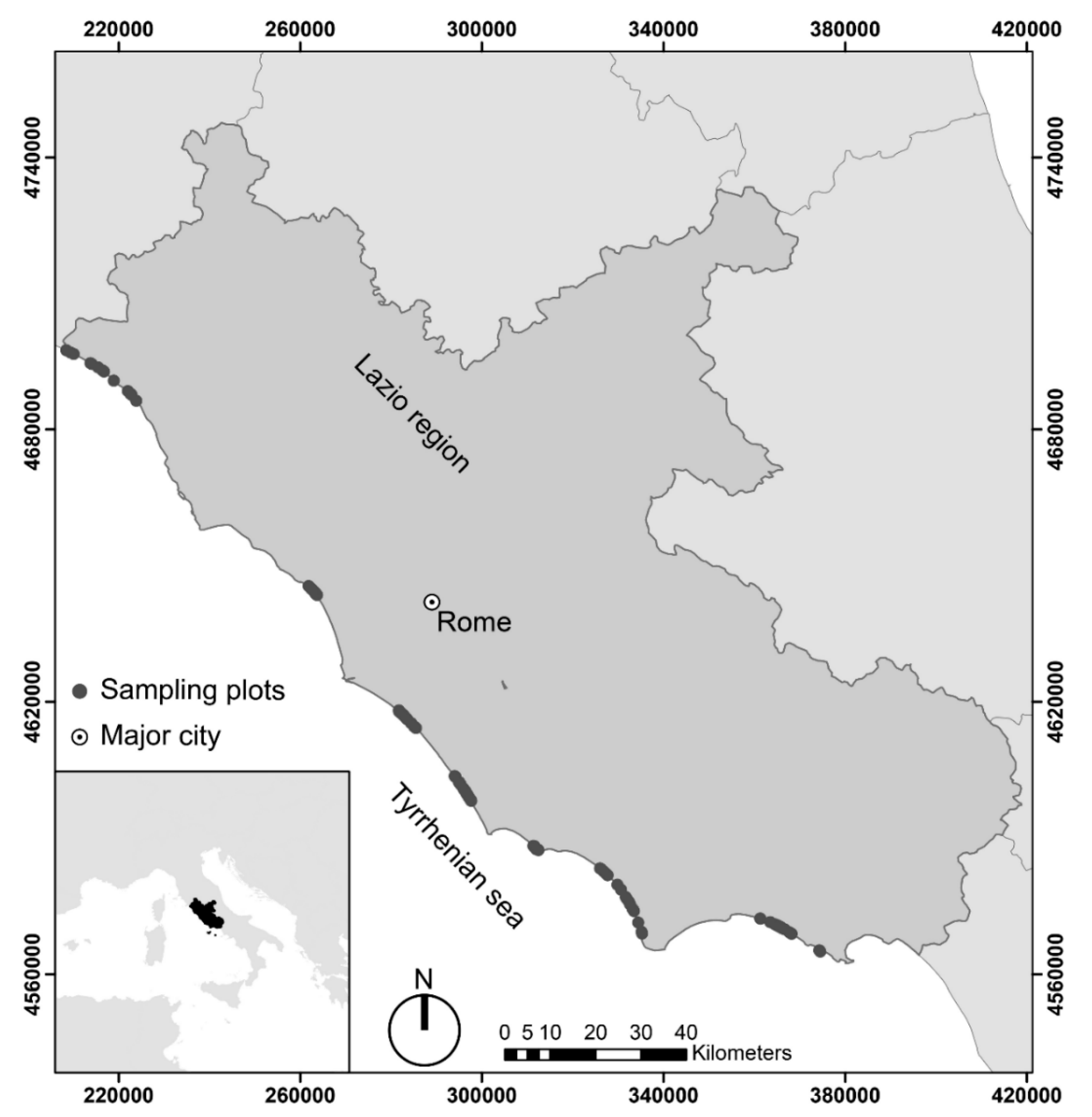
2.1. Study Area

The study was carried out in a coastal tract representative of the Tyrrhenian dunes in central Italy (Lazio region, Figure 1). The sampled sector, approximately 70 km long, includes low sandy Holocenic dunes with Mediterranean climate [47] disposed on a narrow strip along the seashore (<500 m) [28]. In natural conditions, plant communities on shifting dunes are dominated by few dune-building perennial rhizomatous grasses (e.g., Elymus farctus, Ammophila arenaria subsp. australis), which occasionally form monospecific vegetation patches. Plant communities on fixed dunes are characterized by small chamaephytes (e.g., Crucianella maritima) intermingled with species-rich therophytic grasslands (e.g., Cutandia maritima, Lagurus ovatus) [48,49]. As on most of the Mediterranean coasts, the analyzed dunes have undergone persistent human pressure that altered coastal landscapes and vegetation [49,50], with several sectors having been invaded by the iceplant (Carpobrotus spp.) [51,52]. Carpobrotus spp. is a perennial herb with succulent leaves that develops wide creeping mats [51]. It is native of South Africa and, along the Italian sand coasts, it preferentially invades herbaceous vegetation of shifting and fixed dunes [37,53,54]. Field research evidenced that Carpobrotus spp. invasion substantially alters ecosystems diversity [52,55] and functioning of invaded areas [51,56], with such variations being also detectable by RS spectral values [57,58].

2.2. Data Collection and Analysis

We tested the spectral variability hypothesis (SVH) for alpha and beta diversity in coastal dunes following a sequence of steps schematically reported in Figure 2: (1) Data setting, (2) Alpha diversity analysis, (3) Beta diversity analysis, (4) spectral variability hypothesis test.

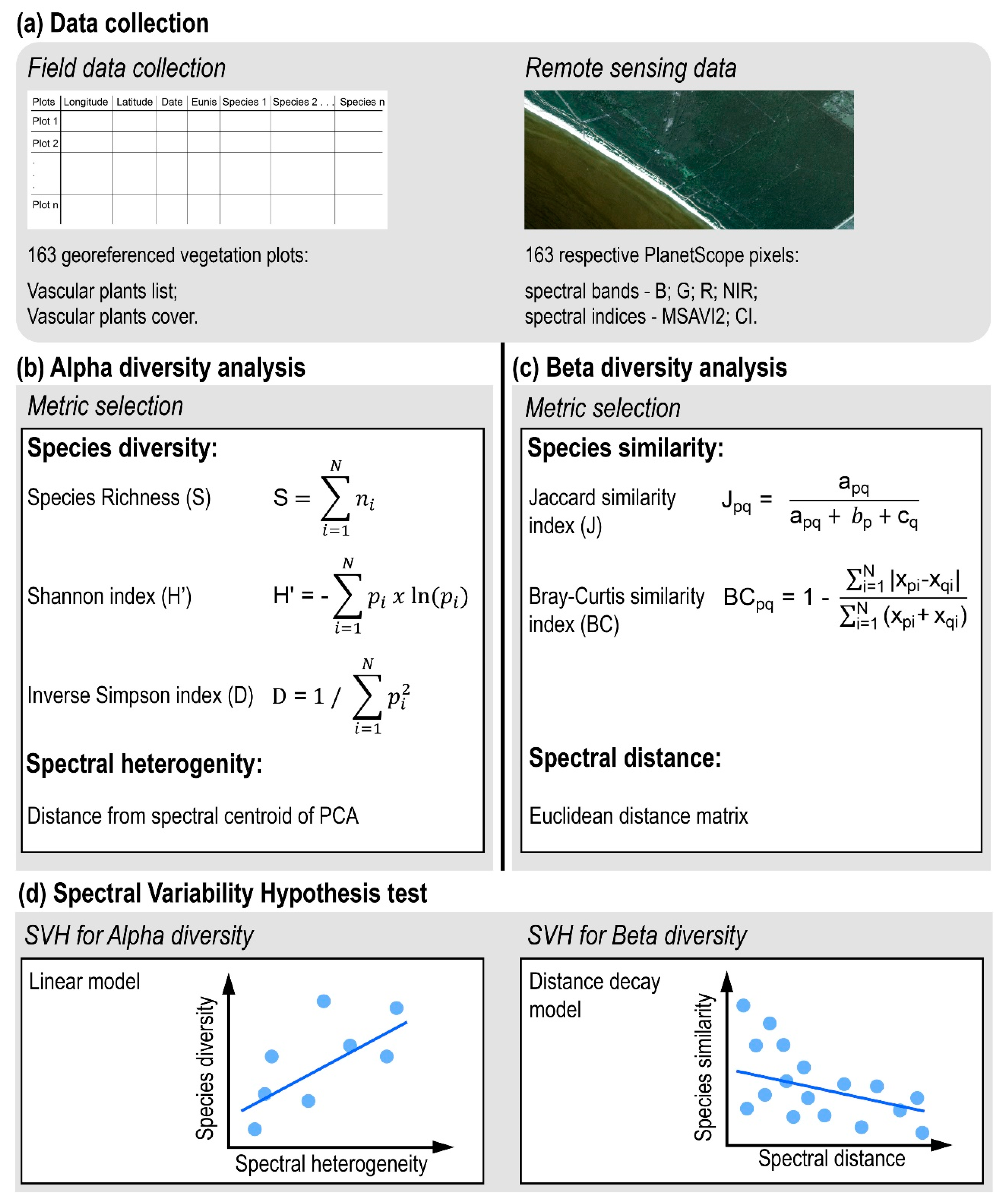
2.2.1. Data Collection

Field Data Collection

We selected biodiversity field data consisting in a set of georeferenced vegetation plots lately collected (years 2017–2020) and stored in the “RanVegDunes” database [59,60] and for which coeval remote sensed images (PlanetScope) were available (Figure 2, box a and b). Specifically field biodiversity data consisted on 163 random 2 × 2 m vegetation plots sampled during the growing seasons (April–May) reporting a complete list of vascular plant species along with their cover in percent. Each plot was also assigned to a EUNIS (European Nature Information System) habitat category, a comprehensive Pan-European classification scheme [60] holding an exact correspondence with European Habitats sensu 92/43/EEC (Table 1), which assured the usefulness of our results to develop new habitat-specific monitoring strategies. Overall, the field floristic data include 79 plots collected on shifting coastal dunes (Shifting dunes, EUNIS code N14), 41 plots on fixed coastal dune (Transition dunes, EUNIS code N16) and 43 invaded plots in which Carpobrotus spp. covers more than 25% (Invaded dunes, Table 1).

Remote-Sensing Data

We selected as RS diversity data the set of pixels with the same geographic coordinates and date of the vegetation plots (Figure 2, box a and b). We extracted RS data from 12 cloud-free PlanetScope (PS) satellite images (zenith angle view <10°; size 3 m, https://www.planet.com/explorer/ (accessed on 28 November 2020), Table S1). We adopted the surface reflectance of the orthorectified PS images (level 3B).
We used for the analysis four spectral bands: blue (B, 455–515 nm), green (G, 500–590 nm), red (R, 590–670 nm), and near infrared (NIR, 780–860) [61] and two spectral indices: Modified Soil-Adjusted Vegetation Index 2 (MSAVI2) and Coloration Index (CI, Table 2). The selected spectral indices are particularly appropriate for describing and mapping heterogeneous landscapes where vegetation and bare surfaces are intermingled [62] as is the case of well-preserved and altered coastal dunes invaded by Carpobrotus spp. [57,58]. MSAVI2 is especially useful for quantifying the photosynthetic biomass in landscapes characterized by high percentages of bare surfaces [62,63,64]. It ranges from −1 (absence of vegetation biomass) to 1 (maximum of vegetation biomass), with higher values indicating higher percentages of photosynthetic biomass [63,65]. CI is a color soil index used to characterize soil conditions [66] and to reveal the organic content in arid soils by the green–red reflectance ratio [67]. This index ranges from −1 to 1, with higher values indicating darker coloration [68].
We built up the spectral dataset (Figure 2, box a) by extracting for each vegetation plot the respective pixel PS value of blue, green, red and NIR spectral bands, and of the derived MSAVI2, and CI spectral indices (Table 2). Pixels were classified according with their respective field plot EUNIS (e.g., “Shifting dunes”-EUNIS-N14, “Transition dunes” -EUNIS-N16) or altered (“Invaded dunes”) category.

2.2.2. Alpha Diversity Analysis

Alpha diversity summarizes the variability within sampling units and can be expressed as richness (i.e., the number of item types) and evenness (i.e., items’ relative abundance) [69,70]. As sampling units, we considered the vegetation plots for field dataset and the corresponding pixels for spectral information.
We analyzed alpha diversity from field data using three indices (Figure 2, box b; Table 3): species richness (S), Shannon (H’) and inverse Simpson index (D) [71], through the “BiodiversityR” R package (function diversityresult) [72]. Species Richness quantifies the count of species inside plots [73], while Shannon diversity (H’) accounts for the number of species and their relative evenness [19,74,75]. The Shannon index varies from 0 in plots with one dominant species to an undetermined maximum in plots with equally abundant species [71]. The Simpson index, also called “dominance index”, summarizes species richness and dominance. The inverse Simpson index (D) is the reciprocal of the Simpson index, and ranges from one in plots with only one species to an undetermined maximum in plots with all individuals belonging to different species [71,76,77].
We expressed the RS alpha diversity as the distance from the spectral centroid index (Figure 2, box b) [9,14]. Specifically, we calculated the mean distance of all the sampled pixels from the principal component analysis (PCA) centroid built on pixels’ spectral values (B, G, R, NIR, MSAVI2 and CI) [14,75]. Higher values of the distance from the spectral centroid index indicates higher pixel spectral heterogeneity [14]. The PCA of the spectral dataset, the identification of the spectral centroid and the calculation of the Euclidean distance from the spectral centroid, were performed using R package “pracma” (function distmat) [78].

2.2.3. Beta Diversity Analysis

Beta diversity depicts the variation among sampling units in both composition and abundance values [69,70]. For beta diversity analysis, we considered as sampling units the vegetation plots (species presence and abundance) and the corresponding pixels (spectral bands and indices values).
Beta diversity in field data was analyzed using two different pairwise measures: the Jaccard similarity matrix using plant occurrence (presence/absence data), and the Bray–Curtis similarity matrix based on abundance values (species cover). Jaccard similarity index (J) quantifies the pairwise similarity between vegetation plots as the ratio between the number of species in common and the number of species that are unique to each plot. J values scoring as zero indicate total inequality among plots, while the total equality is identified by J values of one (Table 4) [79,80]. The Bray–Curtis similarity index (BC) depicts the vegetation plots pairwise differences using quantitative species cover data [71,81]. The BC dissimilarity is defined as the ratio between the difference of abundance values and the sum of abundance values for each species. We calculated the similarity values by subtracting the dissimilarity values to one (Table 4). BC ranges from zero when the plots are completely different to one when the species composition of two plots is identical [82].
Spectral beta diversity was calculated as the pairwise multivariate Euclidean distance of the pixel spectral values [15,20,21]. The Euclidean distance measured the shortest possible distance between two pixels, with higher Euclidean distance values corresponding to higher differences between two pixels in RS bands and spectral indices values [9]. All the spectral dataset variables were standardized to zero mean and unit variance, before moving toward the subsequent analytical steps [20].

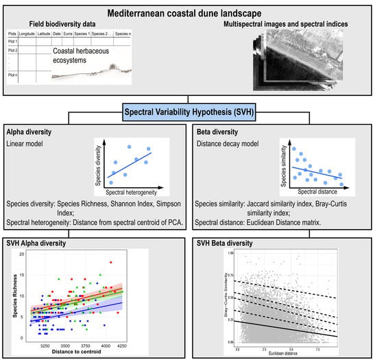
2.2.4. Spectral Variability Hypothesis Test

To test the SVH for alpha diversity, we analyzed the relationship between alpha diversity per plot and spectral heterogeneity for the respective pixels using linear regressions. Specifically, we included in turn plot diversity indices (i.e., species richness, Shannon index and inverse Simpson index) as response variables and the respective pixels’ distance from the spectral centroid index, along with dune well preserved and invaded categories (Shifting, Transition and Invaded dunes, Table 1), as explanatory variables. Goodness-of-fit was evaluated through R2 (Figure 2, box d) [9,19,75]. Since alpha diversity indices are not normally distributed, we fit linear regressions where coefficients significance was evaluated by randomly permuting observations in the data. This approach has the substantial advantage of relaxing the normality assumption of linear regression [83], thus resulting particularly appropriate in our analytical context. Permutational marginal regressions were calculated using the R package “permuco” (function lmperm), allowing 5000 random permutations among observations [84].
To test SVH for beta diversity, we carried out a DDM [85]. In particular, we fit linear regressions and quantile regressions among the floristic Jaccard and Bray–Curtis similarities and the between-pixels Euclidean distances [21]. We tested SVH using both approaches because linear regressions model can be less accurate when based on matrices with a high amount of zeroes, as in our case. The quantile regressions can overcome this limitation and allow to characterize the relationship of SVH by focusing on specific quantiles [85,86]. We calculated the quantile regressions using four upper quantiles (τ = 0.99, 0.95, 0.90, 0.75) according to the hypothesis that maximum decay modelling allows to characterize the maximum beta diversity value [15]. Moreover, higher slopes of the distance decay model indicate higher beta diversity values between samples [12]. Finally, we calculated coefficients confidence intervals for both linear and quantile regressions through a bootstrapping approach (number of iterations: 1000) [21]. We computed the quantile regressions and their confidence intervals using R package “quantreg” (function rq and boot.rq respectively) [87].

3. Results

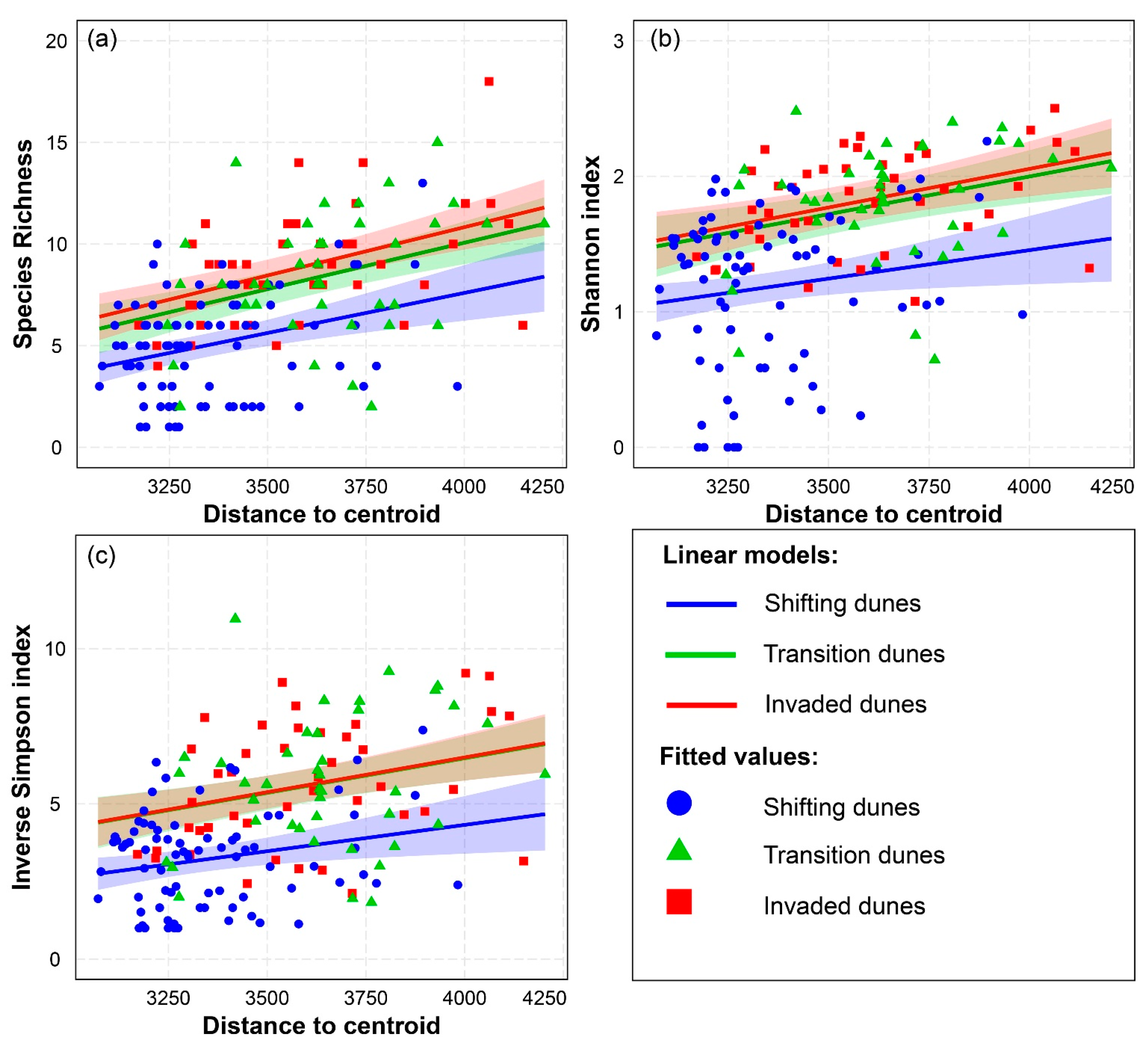
3.1. Spectral Variability Hypothesis (SVH) Alpha Diversity

We observed a significant, positive relationship between species diversity indices and spectral heterogeneity (Figure 3, Table 5) depicting that species diversity values per plot increase toward higher values of spectral heterogeneity per pixel. Among the analyzed alpha diversity indices, Species Richness scored the highest goodness-of-fit (R2 = 0.383), followed by Inverse Simpson index (R2 = 0.342) and Shannon index (R2 = 0.322, Table 5). The interaction effects suggested that the abovementioned positive relationship is true for all the analyzed vegetation types (Shifting, Transition and Invaded dunes, Figure 3). The regression model for species richness showed a highly significant relationship, with positive coefficients for all three vegetation categories (Table 5). Similarly, the models for inverse Simpson and Shannon indices reported significant relationships for the three analyzed vegetation categories (Table 5). Permutation regressions confirmed significant relationships for all the considered alpha diversity indices (Table S2).
In the Cartesian space, the shifting coastal dune vegetation (EUNIS-N14) regression line was below the other categories with significant lower values for species richness (SN14= 1–13), Shannon index (H’N14 = 0.000–2.259) and Inverse Simpson index (DN14 = 1.000–7.376, Figure 3). The regression lines for transition fixed dunes (EUNIS-N16) and invaded vegetation (Invaded dunes) showed similar trends and ranges, slightly differentiating only in species numbers (SN16 = 2–15; SI = 4–18, Figure 3), whereas in both the Shannon index and inverse Simpson index the trends and ranges resulted almost identical (H’N16 = 0.64–2.450, H’I = 1.077–2.502, DN16 = 1.830–10.960, DI = 2.117–9.212).

3.2. SVH Beta Diversity

The distance decay models’ fit with both linear and quantile regressions evidenced negative and significant decay rates (Figure 4, Table 6) for all the categories (i.e., Jaccard floristic similarities vs. Euclidean spectral distance and Bray–Curtis floristic similarities vs. Euclidean spectral distance). Accordingly, the similarity among floristic plots were significantly higher when the respective pixels were spectrally closer.
In the DDM based on Jaccard floristic similarity vs. Euclidean spectral distance, the decay rates showed the lower slope values for linear regression, with slopes increasing until the 0.95 quantile. The slope of 0.99 quantile instead resulted lower than the 0.95 one (Figure 4, Table 6).
The DDM based on Bray–Curtis floristic similarity vs. Euclidean spectral distance showed most intense decay rates at intermediate quantiles (0.90 and 0.95), and the lower rate for the linear regression. The decay rates of the 0.75 and 0.99 quantile showed a intermediate trends respect the others quantiles (Figure 4, Table 6).
In both DDMs, the intercepts of all five regressions indicated significant values with higher values with respect to the linear regression to 0.99 quantile (Figure 4, Table 6). This increasing intercept values confirmed that plots with higher similarity values correspond to pixels with lower spectral distance.
The distribution of fitted values in the DDM (Jaccard floristic similarities vs. Euclidean distance and Bray–Curtis floristic similarities vs. Euclidean distance) differed. Even if the two similarity matrices showed comparable variation ranges (0.000–0.937 for Jaccard similarities matrix, 0.000–0.968 for Bray–Curtis similarities matrix), the measures of central tendency diverged. Indeed, the Jaccard similarity matrix resulted closer to zero (mean: 0.107, median: 0.083, standard deviation: 0.106) than the Bray–Curtis one (mean: 0.179, median: 0.154. standard deviation: 0.157).
When analyzing the DDM separately for the dunes category, the results showed different trends. The significance of decay rates in Shifting dunes (EUNIS-N14) partially confirmed SVH. Examining the Jaccard floristic similarities vs. Euclidean distance the relationships are preserved for the linear regression, 0.75 and 0.90 quantiles, whereas only the decay rate of 0.75 quantile is negative and significant in the Bray–Curtis floristic similarities vs. Euclidean distance models (Table S3, Figure S1). In the transitional Gray dunes (EUNIS-N16) and in the Invaded dunes, the Bray-Curtis floristic similarities vs. Euclidean distance models confirmed the SVH for all regressions with negative and significant decay rates, whereas in Jaccard floristic similarities vs. Euclidean distance models these two categories showed different trends (see Tables S4 and S5, Figures S2 and S3). The transition Gray dunes verified the SVH only for the linear regression, 0.95 and 0.99 quantiles, and the Invaded dunes registered negative and significant decay rates for all models (see Tables S4 and S5, Figures S2 and S3).

4. Discussion

In this study, we provided a first assessment of the relationship between floristic and spectral RS diversity in a highly dynamic landscape, such as coastal dunes. The SVH analysis, suggested the potential of RS spectral data in providing reliable information concerning floristic alpha and beta diversity in well-preserved Mediterranean coastal vegetation (Shifting dunes and Transition dunes) and also on altered dunes invaded by Carpobrotus spp.
The relation between floristic indices of richness, Shannon and inverse Simpson with spectral diversity (distance from the spectral centroid) gave evidence of the potential RS data for monitoring alpha biodiversity [14,88] on heterogeneous and fine grained landscapes as Mediterranean dunes. As observed in other ecosystems as the savannah [19,75] and the evergreen [10] and temperate forests [89], we have registered a positive relation between species and spectral diversity. As noticed by Nagendra et al. [16] on a markedly different environment as dry tropical forests, species richness on coastal vegetation resulted in being related with spectral variability. Furthermore, the observed link of the inverse Simpson and Shannon indices with spectral diversity values extended the field of application of SVH beyond the previous results reported for coarse and homogeneous vegetation types as forests [10] and gave new evidence of the benefit of using RS for monitoring tiny dynamic mosaics as coastal dunes. Similarly, to which was registered by Madonsela et al. [19] on savannah woodlands, also on coastal dunes we observed a similar relation of Inverse Simpson index and Shannon values with spectral diversity. Such results suggest that both: evenness and dominance, have a comparable weight in determining the field vs. RS variability relationship.
Some studies have characterized alpha spectral diversity analyzing pixel values of single bands or indices, losing outstanding information supplied by RS images [16,17,90]. The use of multivariate spectral distance [19,24] had allowed us to capitalize PlanetScope images information for describing coastal landscape variability and to relate it with species diversity. Moreover, the use of spectral bands combined with the estimates of biomass (MSAVI2) and soil organic matter content (CI) [88] supported the potential of SVH for depicting coastal dune vegetation diversity. The consistency of vegetation plots dimension with PlanetScope pixel size, as well as the chosen indices of plant diversity and spectral variability [25,91], further enabled the present application on coastal dune landscapes. Concerning the observed weak goodness-of-fit of linear regressions we considered that as observed by Schmidtlein et al. [25] also in our case it should be likely due to the low spectral resolution of RS (4 spectral bands, and 2 spectral indices).
Concerning beta diversity, the analyzed distance decay models disclosing floristic similarities (Jaccard and Bray–Curtis) and spectral Euclidean distance, showed significant relationships in all quantile regressions and linear regression considering all dunes categories. Our results gave evidence of the effectiveness of the distance decay model to describe coastal landscape beta diversity on natural as well as on invaded dunes. Increasing values in spectral distance concomitant with decreasing floristic similarity were observed in other ecosystems characterized by coarser scales (grain and extent) as temperate [90], tropical [92], and Mediterranean [15] forests. The observed weak decay rates in the linear regression model compared to the quantile regressions is probably related with the high number of zeros in the similarity matrix [21]. It should be noted that the relation among RS spectral Euclidean distances and floristic similarities computed with species abundance are stronger than those computed with the presence/absence of data. The moderate decay rate of 0.99 quantile regressions in both distance decay models is probably due to minor errors on spatial matching between RS PlanetScope images and the field georeferenced plots [21,93]. Analyzing beta diversity separately for each dune habitat, we observed a robust distance decay model on habitat types characterized by continuous vegetation cover (e.g., Transition dunes-EUNIS-N16 and Invaded vegetation), whereas in the Shifting dunes (EUNIS-N14) it is weak. This weak decay trend is probably related with the intrinsic characteristics of shifting dunes given in the field by monospecific or floristically poor plots (low beta diversity) and in RS images by pixels with different degrees of bare soil and sparse vegetation (high between pixel distance). Similar to what was reported by Wang et al. [94] on natural grasslands, the PlanteScope RS spatial resolution seemed too coarse to discriminate some tiny monospecific formations on shifting dunes, thus the RS beta diversity included the variability of reflectance values of pixels hosting Shifting dunes communities with different levels of vegetation cover and bare soil [94].
The SVH analysis for alpha and beta diversity evidenced a similar behavior of Herbaceous vegetation with the presence Carpobrotus spp. and natural dune vegetation (Shifting and Transition coastal dune vegetation). The relation of spectral alpha and beta diversity on Carpobrotus spp. invaded plots is included in the general pattern of the analyzed herbaceous coastal vegetation mosaic (Figure 3, Table 5, see also Table S5, Figure S3). These general biodiversity trends are most likely related with the coastal dune vegetation gradient that, on well preserved plots, ranges from monospecific formations [95] to chamaephytic vegetation intermingled with species-rich therophytic grasslands and on invaded areas to different invasion strengths [51,53,55]. The slightly large confidence intervals observed on shifting dunes (Figure 3) is most likely related with the presence on well-preserved areas of monospecific plots (e.g., Elymus farctus or Ammophila arenaria subsp. australis formations) with low field alpha diversity. The spectral diversity on the respective pixels is influenced by open herbaceous vegetation and bare soil depicting a heterogeneous spectral information and consequently a partially mismatch between field and spectral diversity values. This partial mismatch among monospecific vegetation plots and the respective RS heterogeneous pixels promoted the observed wider variability on shifting dunes compared with the other coastal dune habitats.
Our results underlined the effectiveness of the spectral variability hypothesis for depicting both alpha and beta diversity levels, thus supporting the application of RS data for estimating and monitoring diversity on coastal landscapes. The RS assessment of biodiversity based on the spectral variability hypothesis, which was already proposed for monitoring other ecosystems [17,22,96], can now be extended to highly heterogeneous and dynamic mosaics as coastal dunes even on altered conditions due to plant invasions.
The observed relationship between spectral and floristic diversity in natural and invaded dune vegetation is certainly a first applied outcome of the SVH and support it as a valid approach to better exploring variations in alpha and beta diversity and to improving the early warning systems needed to prevent the biodiversity loss.

5. Conclusions

In this study, we provided a first assessment of the relationship between floristic and spectral RS diversity in Mediterranean coastal dunes’ herbaceous vegetation, extending the applicability of the SVH also in these dynamic landscapes. Such a relationship was analyzed for well-preserved European habitats (sensu 92/43/EEC) and on invaded ecosystems, providing useful insights for improving the biodiversity monitoring and reporting obligations required by the Habitats Directive and supporting field surveys. This research extended the field of applicability of RS for alpha and beta diversity assessment on coastal dunes, as well as gave evidence of the potential of using spectral bands combined with spectral indices to better depict ground biodiversity. This result was made possible by the support of multispectral PlanetScope satellite images (https://www.planet.com/explorer/—accessed on 28 November 2020) which free access have increased the opportunities of monitoring the coastal biodiversity at low cost. Further analysis using RS images with higher spectral resolution (e.g., the open PRISMA (PRecursore IperSpettrale della Missione Applicativa) data funded by the Italian Space Agency ASI), could enhance the potential for discriminating different species [12,14], reinforcing the observed alpha field vs. spectral RS diversity relationship.
These seminal work extends the SVH application to coastal dunes’ taxonomic diversity assessment and suggests the need for additional research to further explore the potential of RS for monitoring other facets of coastal dune diversity as the functional and phylogenetic ones [97,98].

Supplementary Materials

The following are available online at https://www.mdpi.com/article/10.3390/rs13101928/s1, Table S1. PlanetScope images selected accounting of the geographic and temporal distribution of field collected vegetation plots. For each image we reported: the satellite, the date and the hour of acquisition, the product level, the cloud percentage, the zenith angle of acquisition, the coordinate of the center of each multispectral image, the name of cities and geographic area covered and the administrative Province in brackets (RM: Rome; LT: Latina; VT: Viterbo), Table S2. Results of permutation marginal regressions, indicating the significance of estimates in all three linear regressions (species richness–distance to centroid, Shannon index–distance to centroid, inverse Simpson index–distance to centroid) after 5000 permutations. p-value: * <0.05; ** <0.01; *** <0.001, Figure S1. Distance decay models of species similarity, Jaccard (a) and Bray-Curtis (b), versus spectral distance (spectral pairwise Euclidean distance) considering Shifting dunes (N14 EUNIS category). The linear regression is described by solid line, the quantile regressions considering four different τ (from upper to lower lines: 0.99, 0.95, 0.90, 0.75) are reported by dashed lines. Gray dots represent the sampling plots, Table S3. Results of Distance decay models calculated by linear regression model and quantile regression at four different τ values (from upper to lower lines: 0.99, 0.95, 0.9, 0.75), considering the vegetation plots and the pixels of Shifting dunes (N14 EUNIS category). p-value: * <0.05; ** <0.01; *** <0.001, Figure S2. Distance decay models of species similarity, Jaccard (a) and Bray–Curtis (b), versus spectral distance (spectral pairwise Euclidean distance) considering the vegetation plots and the pixels of Transition dunes (N16 EUNIS category. The linear regression is described by solid line, the quantile regressions considering four different τ (from upper to lower lines: 0.99, 0.95, 0.90, 0.75) are reported by dashed lines. Gray dots represent the sampling plots, Table S4. Results of distance decay models calculated by linear regression model and quantile regression at four different τ values (from upper to lower lines: 0.99, 0.95, 0.9, 0.75), considering the vegetation plots and the pixels of Transition dunes (N16 EUNIS category). p-value: * <0.05; ** <0.01; *** <0.001, Figure S3. Distance decay models of species similarity, Jaccard (a) and Bray–Curtis (b), versus spectral distance (Euclidean distance) considering the vegetation plots and the pixels invaded by Carpobrotus spp., Invaded category. The linear regression is described by solid line, the quantile regressions considering four different τ (from upper to lower lines: 0.99, 0.95, 0.90, 0.75) are reported by dashed lines. Gray dots represent the sampling plots, Table S5. Results of distance decay models calculated by linear regression model and quantile regression at four different τ values (from upper to lower lines: 0.99, 0.95, 0.9, 0.75), considering the vegetation plots and the pixels invaded by Carpobrotus spp., Invaded category. p-value: * <0.05; ** <0.01; *** <0.001.

Author Contributions

All authors contributed substantially to the work: F.M., A.T.R.A. and M.L.C. conceived and designed the study; F.M. and S.C. collected the data; F.M., M.D.F., L.F. and M.L.C. analyzed the data; F.M., A.T.R.A. and M.L.C. led the writing of the manuscript; A.T.R.A. and M.L.C. supervised the research. All authors contributed critically to the drafts and gave final approval for publication. All authors have read and agreed to the published version of the manuscript.

Funding

This research received no external funding.

Institutional Review Board Statement

Not applicable.

Informed Consent Statement

Informed consent was obtained from all subjects involved in the study.

Data Availability Statement

Vegetation plots are archived in the database “RanVegDunes” accessible from the “European Vegetation Archive”. The satellite images have been downloaded from PlanetScope archive.

Acknowledgments

This study was carried out with a support of the bilateral program Italy–Israel DERESEMII (Developing state-of-the-art remote sensing tools for monitoring the impact of invasive plant), the Interreg Italia-Croazia CASCADE (CoAStal and marine waters integrated monitoring systems for ecosystems proteCtion AnD management-Project ID 10255941) and the PON-AIM (Programma Operativo Nazionale ricerca e innovazione 2014–2020; ID AIM1897595-2). Special thanks to PlanetScope for providing the access to daily Planet imagery. The Grant of Excellence Departments, MIUR-Italy (ARTICOLO 1, COMMI 314-337 LEGGE 232/2016) is also gratefully acknowledged. We are grateful to the reviewers and the editors for their valuable comments which help us to improve the manuscript.

Conflicts of Interest

The authors declare no conflict of interest.

References

  1. Ceballos, G.; Ehrlich, P.R.; Barnosky, A.D.; García, A.; Pringle, R.M.; Palmer, T.M. Accelerated modern human–induced species losses: Entering the sixth mass extinction. Sci. Adv. 2015, 1, e1400253. [Google Scholar] [CrossRef] [PubMed] [Green Version]
  2. Díaz, S.; Demissew, S.; Carabias, J.; Joly, C.; Lonsdale, M.; Ash, N.; Larigauderie, A.; Adhikari, J.R.; Arico, S.; Báldi, A.; et al. The IPBES conceptual framework—connecting nature and people. Curr. Opin. Environ. Sustain. 2015, 14, 1–16. [Google Scholar] [CrossRef] [Green Version]
  3. Palmer, M.W.; Earls, P.G.; Hoagland, B.W.; White, P.S.; Wohlgemuth, T. Quantitative tools for perfecting species lists. Environmetrics 2002, 13, 121–137. [Google Scholar] [CrossRef]
  4. Vihervaara, P.; Auvinen, A.P.; Mononen, L.; Törmä, M.; Ahlroth, P.; Anttila, S.; Böttcher, K.; Forsius, M.; Heino, J.; Heliola, J.; et al. How essential biodiversity variables and remote sensing can help national biodiversity monitoring. Glob. Ecol. Conserv. 2017, 10, 43–59. [Google Scholar] [CrossRef]
  5. Petrou, Z.I.; Manakos, I.; Stathaki, T. Remote sensing for biodiversity monitoring: A review of methods for biodiversity indicator extraction and assessment of progress towards international targets. Biodivers. Conserv. 2015, 24, 2333–2363. [Google Scholar] [CrossRef]
  6. Del Vecchio, S.; Fantinato, E.; Silan, G.; Buffa, G. Trade-offs between sampling effort and data quality in habitat monitoring. Biodivers. Conserv. 2019, 28, 55–73. [Google Scholar] [CrossRef] [Green Version]
  7. Maccherini, S.; Bacaro, G.; Tordoni, E.; Bertacchi, A.; Castagnini, P.; Foggi, B.; Gennai, M.; Mugnai, M.; Sarmati, S.; Angiolini, C. Enough is enough? Searching for the optimal sample size to monitor european habitats: A case study from coastal sand dunes. Diversity 2020, 12, 138. [Google Scholar] [CrossRef] [Green Version]
  8. Rocchini, D.; Salvatori, N.; Beierkuhnlein, C.; Chiarucci, A.; de Boissieu, F.; Förster, M.; Garzon-Lopez, C.X.; Gillespie, T.W.; Hauffe, H.C.; He, K.S.; et al. From local spectral species to global spectral communities. a benchmark for ecosystem diversity estimate by remote sensing. Ecol. Inform. 2021, 61, 101195. [Google Scholar] [CrossRef]
  9. Rocchini, D.; Boyd, D.S.; Féret, J.B.; Foody, G.M.; He, K.S.; Lausch, A.; Nagendra, H.; Wegmann, M.; Pettorelli, N. Satellite remote sensing to monitor species diversity: Potential and pitfalls. Remote Sens. Ecol. Conserv. 2016, 2, 25–36. [Google Scholar] [CrossRef]
  10. Torresani, M.; Rocchini, D.; Sonnenschein, R.; Zebisch, M.; Marcantonio, M.; Ricotta, C.; Tonon, G. Estimating tree species diversity from space in an alpine conifer forest: The Rao’s Q diversity index meets the spectral variation hypothesis. Ecol. Inform. 2019, 52, 26–34. [Google Scholar] [CrossRef] [Green Version]
  11. Torresani, M.; Rocchini, D.; Sonnenschein, R.; Zebisch, M.; Hauffe, H.C.; Heym, M.; Pretzsch, H.; Tonon, G. Height variation hypothesis: A new approach for estimating forest species diversity with CHM LiDAR data. Ecol. Indic. 2020, 117, 106520. [Google Scholar] [CrossRef]
  12. Rocchini, D.; Hernández-Stefanoni, J.L.; He, K.S. Advancing species diversity estimate by remotely sensed proxies: A conceptual review. Ecol. Inform. 2015, 25, 22–28. [Google Scholar] [CrossRef]
  13. Lausch, A.; Heurich, M.; Magdon, P.; Rocchini, D.; Schulz, K.; Bumberger, J.; King, D.J. A Range of Earth Observation Techniques for Assessing Plant Diversity. In Remote Sensing of Plant Biodiversity, 1st ed.; Cavender-Bares, J., Gamon, J., Townsend, P., Eds.; Springer Nature: Cham, Switzerland, 2020; pp. 309–348. [Google Scholar]
  14. Rocchini, D. Effects of spatial and spectral resolution in estimating ecosystem α-diversity by satellite imagery. Remote Sens. Environ. 2007, 111, 423–434. [Google Scholar] [CrossRef]
  15. Rocchini, D. Distance decay in spectral space in analyzing β-diversity. Int. J. Remote Sens. 2007, 28, 2635–2644. [Google Scholar] [CrossRef]
  16. Nagendra, H.; Rocchini, D.; Ghate, R.; Sharma, B.; Pareeth, S. Assessing plant diversity in a dry tropical forest: Comparing the utility of Landsat and Ikonos satellite images. Remote Sens. 2010, 2, 478–496. [Google Scholar] [CrossRef] [Green Version]
  17. Heumann, B.W.; Hackett, R.A.; Monfils, A.K. Testing the spectral diversity hypothesis using spectroscopy data in a simulated wetland community. Ecol. Inform. 2015, 25, 29–34. [Google Scholar] [CrossRef]
  18. Hall, K.; Reitalu, T.; Sykes, M.T.; Prentice, H.C. Spectral heterogeneity of QuickBird satellite data is related to fine-scale plant species spatial turnover in semi-natural grasslands. Appl. Veg. Sci. 2012, 15, 145–157. [Google Scholar] [CrossRef]
  19. Madonsela, S.; Cho, M.A.; Ramoelo, A.; Mutanga, O. Remote sensing of species diversity using Landsat 8 spectral variables. ISPRS J. Photogramm. 2017, 133, 116–127. [Google Scholar] [CrossRef] [Green Version]
  20. Hoffmann, S.; Schmitt, T.M.; Chiarucci, A.; Irl, S.D.H.; Rocchini, D.; Vetaas, O.R.; Tanase, M.A.; Stéphane, M.; Bouvet, A.; Beierkuhnlein, C. Remote sensing of β-diversity: Evidence from plant communities in a semi-natural system. Appl. Veg. Sci. 2019, 22, 13–26. [Google Scholar] [CrossRef] [Green Version]
  21. Rocchini, D.; Nagendra, H.; Ghate, R.; Cade, B.S. Spectral distance decay: Assessing species beta-diversity by quantile regression. Photogramm. Eng. Remote Sens. 2009, 75, 1225–1230. Available online: http://citeseerx.ist.psu.edu/viewdoc/download?doi=10.1.1.182.369&rep=rep1&type=pdf (accessed on 14 May 2021).
  22. Féret, J.B.; Asner, G.P. Mapping tropical forest canopy diversity using high-fidelity imaging spectroscopy. Ecol. Appl. 2014, 24, 1289–1296. [Google Scholar] [CrossRef] [PubMed]
  23. Khare, S.; Latifi, H.; Rossi, S. Forest beta-diversity analysis by remote sensing: How scale and sensors affect the Rao’s Q index. Ecol. Indic. 2019, 106, 105520. [Google Scholar] [CrossRef]
  24. Gholizadeh, H.; Gamon, J.A.; Helzet, C.J.; Cavender-Bares, J. Multi-temporal assessment of grassland α- and β-diversity using hyperspectral imaging. Ecol. Appl. 2020, 30, e02145. [Google Scholar] [CrossRef]
  25. Schmidtlein, S.; Fassnacht, F.E. The spectral variability hypothesis does not hold across landscapes. Remote Sens. Environ. 2017, 192, 114–125. [Google Scholar] [CrossRef] [Green Version]
  26. Martínez, M.L.; Psuty, N.P. Coastal Dunes. Ecology and Conservation, 1st ed.; Springer: Berlin, Germany, 2004; pp. 3–29. [Google Scholar]
  27. Hesp, P. A Ecological processes and plant adaptations on coastal dunes. J. Arid Environ. 1991, 21, 165–191. [Google Scholar] [CrossRef]
  28. Acosta, A.T.R.; Blasi, C.; Carranza, M.L.; Ricotta, C.; Stanisci, A. Quantifying ecological mosaic connectivity with a new topoecological index. Phytocoenologia 2003, 33, 623–631. [Google Scholar] [CrossRef]
  29. Kim, D.; Yu, K.B. A conceptual model of coastal dune ecology synthesizing spatial gradients of vegetation, soil, and geomorphology. Plant Ecol. 2009, 202, 135–148. [Google Scholar] [CrossRef]
  30. Bazzichetto, M.; Malavasi, M.; Acosta, A.T.R.; Carranza, M.L. How does dune morphology shape coastal EC habitats occurrence? A remote sensing approach using airborne LiDAR on the Mediterranean coast. Ecol. Indic. 2016, 71, 618–626. [Google Scholar] [CrossRef]
  31. McLachlan, A.; Brown, A.C. The Ecology of Sandy Shores, 2nd ed.; Elsevier: Burlington, NJ, USA, 2006; pp. 273–323. [Google Scholar]
  32. Doody, J.P. Sand Dune Conservation, Management and Restoration, 1st ed.; Springer Science: Dordrecht, The Netherlands, 2013; pp. 37–82. [Google Scholar]
  33. Janssen, J.A.M.; Rodwell, J.S.; García Criado, M.; Gubbay, S.; Haynes, T.; Nieto, A.; Sanders, N.; Landucci, F.; Loidi, J.; Ssymank, A.; et al. European Red List of Habitats. Part 2. Terrestrial and Freshwater Habitats, 1st ed.; European Commision: Luxembourg, 2016; pp. 1–40. [Google Scholar]
  34. Prisco, I.; Angiolini, C.; Assini, S.; Buffa, G.; Gigante, D.; Marcenó, C.; Sciandrello, S.; Villani, M.; Acosta, A.T.R. Conservation status of Italian coastal dune habitats in the light of the 4th monitoring report (92/43/EEC Habitats directive). Plant Sociol. 2020, 57, 55–64. [Google Scholar] [CrossRef]
  35. Defeo, O.; McLachlan, A.; Schoeman, D.S.; Schlacher, T.A.; Dugan, J.; Jones, A.; Lastra, M.; Scapini, F. Threats to sandy beach ecosystems: A review. Estuar. Coast. Shelf Sci. 2009, 8, 1–12. [Google Scholar] [CrossRef]
  36. Chytrý, M.; Maskell, L.C.; Pino, J.; Pyšek, P.; Vilà, M.; Font, X.; Smart, S.M. Habitat invasons by alien plants: A quantitative comparison among Mediterranean, subcontinental and oceanic regions of Europe. J. Appl. Ecol. 2008, 45, 448–458. [Google Scholar] [CrossRef]
  37. Lazzaro, L.; Bolpagni, R.; Buffa, G.; Gentili, R.; Lonati, M.; Stinca, A.; Acosta, A.T.R.; Adorni, M.; Aleffi, M.; Allegrezza, M.; et al. Impact of invasive alien plants on native plant communities and Natura 2000 habitats: State of the art, gap analysis and perspectives in Italy. J. Environ. Manag. 2020, 274, 111140. [Google Scholar] [CrossRef] [PubMed]
  38. Tordoni, E.; Bacaro, G.; Weigelt, P.; Cameletti, M.; Janssen, J.A.M.; Acosta, A.T.R.; Bagella, S.; Filigheddu, R.; Bergmeier, E.; Buckley, H.L.; et al. Disentangling native and alien plant diversity in coastal sand dune ecosystems worldwide. J. Veg. Sci. 2020, 32, e12861. [Google Scholar] [CrossRef]
  39. Giulio, S.; Acosta, A.T.R.; Carboni, M.; Campos, J.A.; Chytrý, M.; Loidi, J.; Pergl, J.; Pyšek, P.; Isermann, M.; Janssen, J.A.M.; et al. Alien flora across European coastal dunes. Appl. Veg. Sci. 2020, 23, 317–327. [Google Scholar] [CrossRef]
  40. Royimani, L.; Mutanga, O.; Odindi, J.; Dube, T.; Matonger, T.N. Advancements in satellite remote sensing for mapping and monitoring of alien invasive plant species (AIPs). Phys. Chem. Earth PT A/B/C 2019, 112, 237–245. [Google Scholar] [CrossRef]
  41. Early, R.; Bradley, B.A.; Dukes, J.S.; Lawler, J.J.; Olden, J.D.; Blumenthal, D.M.; Gonzalez, P.; Grosholz, E.D.; Ibañez, I.; Miller, L.P.; et al. Global threats from invasive alien species in the twenty-first century and national response capacities. Nat. Commun. 2016, 7, 12485. [Google Scholar] [CrossRef] [PubMed]
  42. Lambdon, P.W.; Pyšek, P.; Basnou, C.; Hejda, M.; Arianoutsou, M.; Essl, F.; Jarošík, V.; Pergl, J.; Winter, M.; Anastasiu, P.; et al. Alien flora of Europe: Species diversity, temporal trends, geographical patterns and research needs. Preslia 2008, 80, 101–149. [Google Scholar]
  43. Niphadkar, M.; Nagendra, H. Remote sensing of invasive plants: Incorporating functional traits into the picture. Int. J. Remote Sens. 2016, 37, 3074–3085. [Google Scholar] [CrossRef]
  44. Guisan, A.; Petitpierre, B.; Broennimann, O.; Daehler, C.; Kueffer, C. Unifying niche shift studies: Insights from biological invasions. Trends Ecol. Evol. 2014, 29, 260–269. [Google Scholar] [CrossRef] [Green Version]
  45. Drius, M.; Jones, L.; Marzialetti, F.; de Francesco, M.C.; Stanisci, A.; Carranza, M.L. Not just a sandy beach. The multi-service value of Mediterranean coastal dunes. Sci. Total Environ. 2019, 668, 1139–1155. [Google Scholar] [CrossRef] [Green Version]
  46. Viciani, D.; Vidali, M.; Gigante, D.; Bolpagni, R.; Villani, M.; Acosta, A.T.R.; Adorni, M.; Aleffi, M.; Allegrezza, M.; Angiolini, C.; et al. A first checklist of the alien-dominated vegetation in Italy. Plant Sociol. 2020, 57, 29–54. [Google Scholar] [CrossRef]
  47. Carranza, M.L.; Acosta, A.T.R.; Stanisci, A.; Pirone, G. Ecosystem classification for EU habitat distribution assessment in sandy coastal environments: An application in central Italy. Environ. Monit. Assess. 2008, 140, 99–107. [Google Scholar] [CrossRef] [PubMed]
  48. Acosta, A.T.R.; Carranza, M.L.; Izzi, C.F. Are there habitats that contribute best to plant species diversity in coastal dunes? Biodivers. Conserv. 2009, 18, 1087–1098. [Google Scholar] [CrossRef]
  49. Sperandii, M.G.; Barták, V.; Acosta, A.T.R. Effectiveness of the Natura 2000 network in conserving Mediterranean coastal dune habitats. Biol. Conserv. 2020, 248, 108689. [Google Scholar] [CrossRef]
  50. Malavasi, M.; Santoro, R.; Cutini, M.; Acosta, A.T.R.; Carranza, M.L. The impact of human pressure on landscape patterns and plant species richness in Mediterranean coastal dunes. Plant Biosyst. 2016, 150, 73–82. [Google Scholar] [CrossRef]
  51. Campoy, J.G.; Acosta, A.T.R.; Affre, L.; Barreiro, R.; Brundu, G.; Buisson, E.; González, L.; Buisson, E.; González, L.; Lema, M. Monographs of invasive plants in Europe: Carpobrotus. Bot. Lett. 2018, 165, 440–475. [Google Scholar] [CrossRef]
  52. Sarmati, S.; Conti, L.; Acosta, A.T.R. Carpobrotus acinaciformis vs Carpobrotus edulis: Are there any differences in their impact on coastal dune plant biodiversity? Flora 2019, 257, 151422. [Google Scholar] [CrossRef]
  53. Carranza, M.L.; Carboni, M.; Feola, S.; Acosta, A.T.R. Landscape-scale patterns of alien plant species on coastal dune: The case of iceplant in central Italy. Appl. Veg. Sci. 2010, 13, 135–145. [Google Scholar] [CrossRef]
  54. Bazzichetto, M.; Malavasi, M.; Barták, V.; Acosta, A.T.R.; Moudrý, V.; Carranza, M.L. Modeling plant invasion on Mediterranean coastal landscapes: An integrative approach using remotely sensed data. Landsc. Urban Plan. 2018, 171, 98–106. [Google Scholar] [CrossRef]
  55. Santoro, R.; Jucker, T.; Carranza, M.L.; Acosta, A.T.R. Assessing the effects of Carpobrotus invasion on coastal dune soils. Does the nature of the invaded habitat matter? Community Ecol. 2011, 12, 234–240. [Google Scholar] [CrossRef]
  56. Conser, C.; Connor, E.F. Assessing the residual effects of Carpobrotus edulis invasion, implications for restoration. Biol. Invasions 2009, 11, 349–358. [Google Scholar] [CrossRef]
  57. Underwood, E.; Ustin, S.L.; Di Pietro, D. Mapping nonnative plants using hyperspectral imagery. Remote Sens. Environ. 2003, 86, 150–161. [Google Scholar] [CrossRef]
  58. Underwood, E.; Ustin, S.L.; Ramirez, C.M. A comparison of spatial and spectral image resolution for mapping invasive plants in coastal California. Environ. Manag. 2007, 39, 63–83. [Google Scholar] [CrossRef]
  59. Sperandii, M.G.; Prisco, I.; Stanisci, A.; Acosta, A.T.R. RanVegDunes-A random plot database of Italian coastal dunes. Phytocoenologia 2017, 47, 231–232. [Google Scholar] [CrossRef]
  60. Chytrý, M.; Tichý, L.; Hennekens, S.M.; Knollová, I.; Janssen, J.A.M.; Rodwell, J.S.; Peterka, T.; Marcenò, C.; Landucci, F.; Danihelka, J.; et al. EUNIS habitat classification: Expert system, characteristic species combinations and distribution maps of European habitats. Appl. Veg. Sci. 2020, 23, 1–28. [Google Scholar] [CrossRef]
  61. Cooley, S.W.; Smith, L.C.; Stepan, L.; Mascaro, J. Tracking dynamic northern surface water changes with high-frequency Planet CubeSat imagery. Remote Sens. 2017, 9, 1306. [Google Scholar] [CrossRef] [Green Version]
  62. Marzialetti, F.; Di Febbraro, M.; Malavasi, M.; Giulio, S.; Acosta, A.T.R.; Carranza, M.L. Mapping coastal dune landscape through spectral Rao’s Q temporal diversity. Remote Sens. 2020, 12, 2315. [Google Scholar] [CrossRef]
  63. Qi, J.; Chehbouni, A.; Huete, A.R.; Kerr, Y.H.; Sorooshian, S.A. A modified soil adjusted vegetation index. Remote Sens. Environ. 1994, 48, 118–126. [Google Scholar] [CrossRef]
  64. Wu, Z.; Velasco, M.; McVay, J.; Middleton, B.; Vogel, J.; Dye, D. MODIS derived vegetation index for drought detection on the San Carlos Apache reservation. Int. J. Adv. Remote Sens. GIS 2016, 5, 1524–1538. [Google Scholar] [CrossRef] [Green Version]
  65. Rondeaux, G.; Steven, M.; Baret, F. Optimization of soil-adjusted vegetation indices. Remote Sens. Environ. 1996, 55, 55–107. [Google Scholar] [CrossRef]
  66. Mathieu, R.; Pouget, M.; Cervelle, B.; Escadafal, R. Relationships between satellite-based radiometric indices simulated using laboratory reflectance data and typic soil colour of an arid environment. Remote Sens. Environ. 1998, 66, 17–28. [Google Scholar] [CrossRef]
  67. Bachaoui, B.; Bachaoui, E.M.; Maimouni, S.; Lhissou, R.; El Harti, A.; El Ghmari, A. The use of spectral and geomorphometric data for water erosion mapping in El Ksiba region in the central High Atlas Mountains of Morocco. Appl. Geomat. 2014, 6, 159–169. [Google Scholar] [CrossRef]
  68. Escadafal, R. Remote sensing of soil color: Principles and applications. Remote Sens. Rev. 1993, 7, 261–279. [Google Scholar] [CrossRef]
  69. Whitaker, R.H. Vegetation of the Siskiyou Mountains, Oregon and California. Ecol. Monogr. 1960, 30, 279–338. [Google Scholar] [CrossRef]
  70. Whitaker, R.H. Evolution and measurement of species diversity. Taxon 1972, 21, 213–251. [Google Scholar] [CrossRef] [Green Version]
  71. Magurran, A.E. Measuring Biological Diversity, 1st ed.; Blackwell Science: Maden, NJ, USA, 2004; pp. 100–185. [Google Scholar]
  72. Kindt, R.; Coe, R. Tree Diversity Analysis. A Manual and Software for Common Statistical Methods for Ecological and Biodiversity Studies, 1st ed.; World Agroforestry Centre (ICRAF): Nairobi, Kenya, 2005; pp. 31–70. [Google Scholar]
  73. Fisher, R.A.; Corbet, A.S.; Williams, C.B. The relation between the number of species and the number of individuals in a random sample of an animal population. J. Anim. Ecol. 1943, 12, 42–58. [Google Scholar] [CrossRef]
  74. Shannon, C.E. A mathematical theory of communication. Bell Syst. Tech. J. 1948, 23, 379–423. [Google Scholar] [CrossRef] [Green Version]
  75. Oldeland, J.; Wesuls, D.; Rocchini, D.; Schmidt, M.; Jürgens, N. Does using species abundance data improve estimates of species diversity from remotely sensed spectral heterogeneity? Ecol. Indic. 2010, 10, 390–396. [Google Scholar] [CrossRef]
  76. Peet, R.K. The measurement of species diversity. Annu. Rev. Ecol. Syst. 1974, 5, 285–307. [Google Scholar] [CrossRef]
  77. Jost, L. Partitioning diversity into independent alpha and beta components. Ecology 2007, 88, 2427–2439. [Google Scholar] [CrossRef] [Green Version]
  78. Borchers, H.W. Pracma: Pratical Numerical Math Functions, R Package Version 2.2.9. 2019. Available online: https://cran.r-project.org/web/packages/pracma/index.html (accessed on 15 October 2020).
  79. Jaccard, P. Étude comparative de la distribution florale dans une portion des Alpes et du Jura. Bull. de la Société Vaud. des Sci. Nat. 1901, 37, 547–579. [Google Scholar]
  80. Wildi, O. Data Analysis in Vegetation Ecology, 1st ed.; John Wiley & Sons: Chichester, UK, 2010; pp. 25–34. [Google Scholar]
  81. Bray, J.R.; Curtis, J.T. An ordination of the upland forest communities of Southern Wisconsin. Ecol. Monogr. 1957, 27, 325–349. [Google Scholar] [CrossRef]
  82. Pavoine, S.; Ricotta, C. Measuring functional dissimilarity among plots: Adapting old methods to new questions. Ecol. Indic. 2019, 97, 67–72. [Google Scholar] [CrossRef]
  83. Anderson, M.J.; Robinson, J. Permutation Tests for Linear Models. Aust. N. Z. J. Stat. 2001, 43, 75–88. [Google Scholar] [CrossRef]
  84. Frossard, J.; Renaud, O. Permuco: Permutation Tests for Regression, (Repeated Measures) ANOVA/ANCOVA and Comparison of Signals, R Package Version 1.1.0. 2019. Available online: https://cran.r-project.org/web/packages/permuco/index.html (accessed on 23 November 2020).
  85. Cade, B.S.; Noon, B.R. A gentle introduction to quantile regression for ecologists. Front. Ecol. Environ. 2003, 1, 412–420. [Google Scholar] [CrossRef]
  86. Henning, S.K.; Estrup, H.A.; Kathrin, K. Rejecting the mean: Estimating the response of fen plant species to environmental factors by non-linear quantile regression. J. Veg. Sci. 2005, 16, 373–382. [Google Scholar] [CrossRef]
  87. Koenker, R. Quantreg: Quantile Regression, R Package Version 5.73. 2020. Available online: https://cran.r-project.org/web/packages/quantreg/index.html (accessed on 10 November 2020).
  88. Warren, S.D.; Alt, M.; Olson, K.D.; Irl, S.D.H.; Steinbauer, M.J.; Jentsch, A. The relathionship between the spectral diversity of satellite imagery habitat heterogeneity, and plant species richness. Ecol. Inform. 2014, 24, 160–168. [Google Scholar] [CrossRef]
  89. Meng, J.; Li, S.; Wang, W.; Liu, Q.; Xie, S.; Ma, W. Estimation of forest structural diversity using the spectral and textural information derived from SPOT-5 satellite images. Remote Sens. 2016, 8, 125. [Google Scholar] [CrossRef] [Green Version]
  90. Arekhi, M.; Yilmaz, O.Y.; Yilmaz, H.; Akyüz, Y.F. Can tree species diversity be assessed with Landsat data in a temperate forest? Environ. Monit. Assess. 2017, 189, 586. [Google Scholar] [CrossRef] [PubMed]
  91. Rocchini, D.; McGlinn, D.; Ricotta, C.; Neteler, M.; Wohlgemuth, T. Landscape complexity and spatial scale influence the relathionship between remotely sensed spectral diversity and survey-based plant species richness. J. Veg. Sci. 2011, 22, 688–698. [Google Scholar] [CrossRef]
  92. Draper, F.C.; Baraloto, C.; Brodrick, P.G.; Phillips, O.L.; Martinez, R.V.; Honorio Coronado, E.N.; Baker, T.R.; Zárate Gómez, R.; Amasifuen Guerra, C.A.; Flores, M.; et al. Imaging spectroscopy predicts variable distance decay across contrasting Amazonian tree communities. J. Ecol. 2018, 107, 696–710. [Google Scholar] [CrossRef]
  93. Xu, Y.; Dickson, B.G.; Hampton, H.M.; Sisk, T.D.; Palumbo, J.A.; Prather, J.W. Effects of mismatches of scale and location between predictor and response variables on forest structure mapping. Photogramm. Engin. Remote Sens. 2009, 75, 313–322. [Google Scholar] [CrossRef]
  94. Wang, R.; Gamon, J.A.; Cavender-Bares, V.; Townsend, P.A.; Zygielbaum, A.I. The spatial sensitivity of the spectral diversity-biodiversity relationship: An experimental test in a prairie grassland. Ecol. Appl. 2018, 28, 541–556. [Google Scholar] [CrossRef] [Green Version]
  95. Acosta, A.T.R.; Ercole, V.; Stanisci, A.; De Patta Pillar, V.; Blasi, C. Coastal vegetation zonation and dune morphology in some Mediterranean ecosystems. J. Coast. Res. 2007, 23, 1518–1524. [Google Scholar] [CrossRef] [Green Version]
  96. Hernández-Stefanoni, J.L.; Gallardo-Cruz, J.A.; Meave, J.A.; Rocchini, D.; Bello-Pineda, J.; López-Martínez, J.O. Modeling α- and β-diversity in a tropical forest from remotely sensed and spatial data. Int. J. Appl. Earth Obs. 2012, 19, 359–368. [Google Scholar] [CrossRef]
  97. Meireles, J.E.; Cavender-Bares, J.; Townsend, P.A.; Ustin, S.; Gamon, J.A.; Schweiger, A.K.; Schaepman, M.E.; Asner, G.P.; Martin, R.E.; Singh, A.; et al. Leaf reflectance spectra capture the evolutionary history of seed plants. New Phytol. 2020, 228, 485–493. [Google Scholar] [CrossRef]
  98. Schweiger, A.K.; Cavender-Bares, J.; Townsend, P.A.; Hobbie, S.E.; Madritch, M.D.; Wang, R.; Tilman, D.; Gamon, J.A. Plant spectral diversity integrates functional and phylogenetic components of biodiversity and predicts ecosystem function. Nat. Ecol. Evol. 2018, 2, 976–982. [Google Scholar] [CrossRef]
Figure 1. Study area (reference system WGS84 33N, epsg: 32633) along with sampling plots.
Remotesensing 13 01928 g001
Figure 2. Workflow describing the procedure followed for investigating the potential of the spectral variability hypothesis for depicting alpha and beta diversity levels on herbaceous coastal dune vegetation.
Remotesensing 13 01928 g002
Figure 3. Linear regression models of alpha floristic diversity: species richness (a), Shannon (b) and inverse Simpson (c) vs. spectral heterogeneity: mean distance from spectral principal component analysis (PCA) centroid. Shifting dunes: N14 EUNIS category; Transition dunes: N16 EUNIS category: Invaded dunes: coastal dune vegetation with the presence Carpobrotus sp. covering more than 25 percent.
Remotesensing 13 01928 g003
Figure 4. Distance decay models of Jaccard (a) and Bray–Curtis (b) species similarity versus spectral distance (spectral pairwise Euclidean distance). The linear regression is described by solid line, the quantile regressions considering four different τ (from upper to lower lines: 0.99, 0.95, 0.90, 0.75) are reported by dashed lines. Gray dots represent the sampling plots.
Remotesensing 13 01928 g004
Table 1. Description of herbaceous dune communities referred to EUNIS (European Nature Information Systems) categories, along with their corresponding European Union (EU) habitat (ex Annex I 92/43/EEC) and the respective number of sampling plots. Coastal dune vegetation with the presence Carpobrotus sp. covering more than 25% are also reported.
Acronym/Vegetation CategoriesDescription and Correspondence with EU Habitats (Ex Annex I 92/43/EEC)Number of Plots
Shifting dunes/EUNIS-N14Mobile coastal sand ridges including embryonic dunes characterized by Elymus farctus and semi-permanent dune systems dominated by Ammophila arenaria subsp. australis (EU habitat code: 2110, 2120).79
Transition dunes/EUNIS-N16Fixed dune grasslands including chamaephytic communities of the inland dunes dominated by Crucianella maritima and annual species-rich communities colonizing dry interdunal depressions. (EU habitat code: 2210, 2230).41
Invaded dunesHerbaceous vegetation with the presence Carpobrotus spp. covering more than 25 percent.43
Table 2. Spectral variables selected for analyzing alpha and beta spectral diversity along with their related bandwidth/equation, index proxy and references.
AcronymNameBandwidth/EquationIndex ofReference
BBlue band455–515 nm[61]
GGreen band500–590 nm[61]
RRed band590–670 nm[61]
NIRNear Infrared band780–860 nm[61]
MSAVI2Modified Soil Adjusted Vegetation Index 2 2 NIR + 1 ( 2 NIR + 1 ) 2 8 ( NIR RED ) 2 photosynthetic biomass[63]
CIColouration index RED     GREEN RED + GREEN organic content level in soil[66]
Table 3. Alpha diversity indices used for analyzing field vegetation data along with the formula and references. N = total number of species; ni = each species; pi = abundance value of i-species.
AcronymNameFormulaReferences
SSpecies Richness i = 1 N n i   [73]
H’Shannon index   i = 1 N p i   x   ln ( p i ) [74]
DInverse Simpson index 1 / i = 1 N p i 2 [76]
Table 4. Beta diversity indices used for analyzing field floristic data along with the formula and references. In the Jaccard similarity between plots (p, q), a = number of species shared between p and q vegetation plots, b = number of unique species in the p vegetation plot, c = number of unique species in q plot. In the Bray–Curtis similarity between plots (p, q), xpi = the abundance value of the i-species on plot p and xqi the abundance value of the i-species on plot q.
AcronymNameFormulaReferences
JJaccard similarity index a p q a p q + b p + c q [79]
BCBray-Curtis similarity index 1     i = 1 n | x pi x qi | i = 1 n ( x pi + x qi ) [81]
Table 5. Summary of linear regressions for alpha floristic diversity (species richness, Shannon and inverse Simpson) vs. spectral heterogeneity (distance from spectral centroid index). Shifting dunes: N14 EUNIS category; Transition dunes: N16 EUNIS category: Invaded dunes: coastal dune vegetation with the presence Carpobrotus sp. covering more than 25%. p-value: * <0.05; ** <0.01; *** <0.001.
Species Richness—Distance to CentroidR2 = 0.383
Linear Model with InteractionsEstimateStd. Errorp-Value
Distance to centroid: Shifting dunes3.937 × 10−39.512 × 10−45.362 × 10−5 ***
Distance to centroid: Transition dunes4.554 × 10−38.794 × 10−46.666 × 10−7 ***
Distance to centroid: Invaded dunes4.746 × 10−38.903 × 10−43.311 × 10−7 ***
Shannon Index—Distance to CentroidR2 = 0.322
Linear Model with InteractionsEstimateStd. Errorp-Value
Distance to centroid: Shifting dunes4.202 × 10−41.754 × 10−40.018 *
Distance to centroid: Transition dunes5.556 × 10−41.622 × 10−47.697 × 10−4 ***
Distance to centroid: Invaded dunes5.702× 10−41.642 × 10−46.624 × 10−4 ***
Inverse Simpson Index—Distance to CentroidR2 = 0.342
Linear Model with InteractionsEstimateStd. Errorp-value
Distance to centroid: Shifting dunes1.695 × 10−36.450 × 10−49.426 × 10−3 **
Distance to centroid: Transition dunes2.231 × 10−35.963 × 10−42.547 × 10−4 ***
Distance to centroid: Invaded dunes2.239 × 10−36.038 × 10−42.885 × 10−4 ***
Table 6. Results of distance decay models calculated by linear and quantile regressions at four different τ values (from upper to lower lines: 0.99, 0.95, 0.9, 0.75). p-value: *** < 0.001.
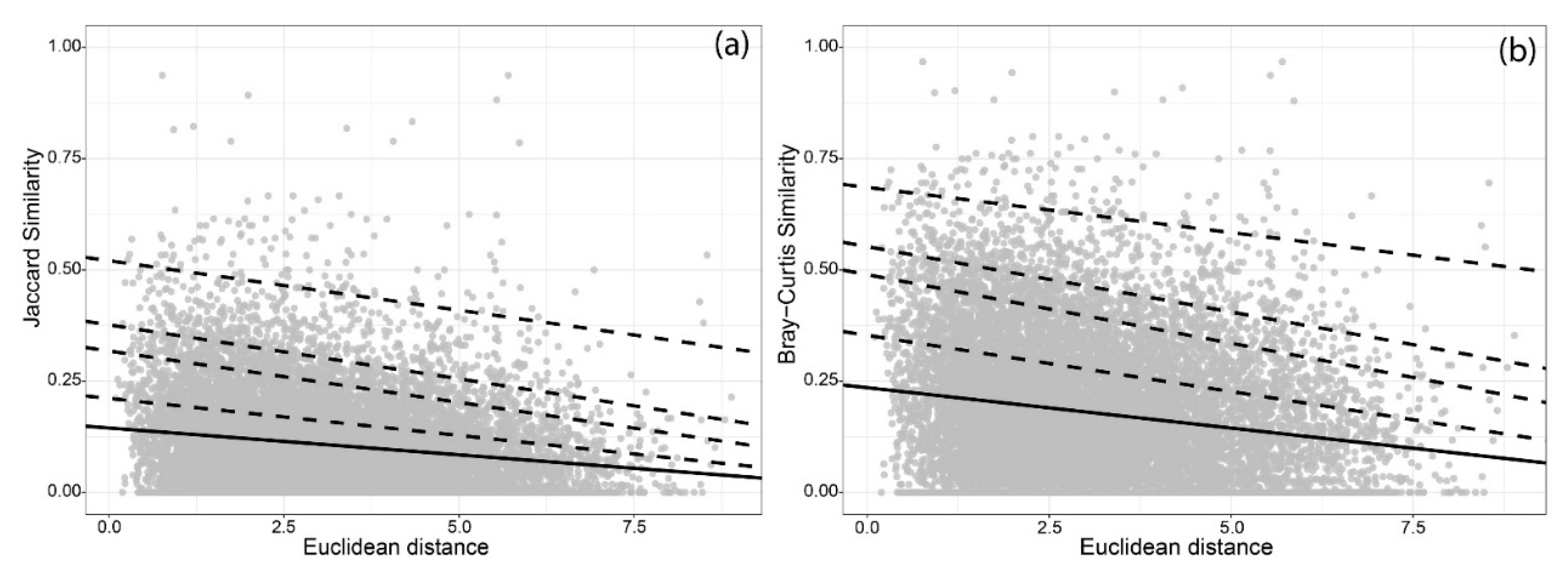
Jaccard Similarities—Uclidean Distance
Regression TypeτInterceptIntercept Boundaries (99%)Decay Rate (10−2)Decay Rate (10−2) Boundaries (99%)
Linea regression0.145 ***0.138–0.152−1.207 ***−1.405–−1.009
Quantile regressions0.750.211 ***0.202–0.220−1.665 ***−1.892–−1.412
0.900.318 ***0.306–0.330−2.312 ***−2.655–−2.009
0.950.377 ***0.361–0.393−2.426 ***−2.83–−1.927
0.990.521 ***0.491–0.564−2.226 ***−3.208–−0.849
Bray-Curtis Similarities—Euclidean Distance
Regression TypeτInterceptIntercept Boundaries (99%)Decay Rate (10−2)Decay Rate (10−2) Boundaries (99%)
Linear regression0.235 ***0.207–0.257−1.814 ***−2.106–−1.522
Quantile0.750.353 ***0.339–0.367−2.529 ***−2.867–−2.200
0.900.489 ***0.473–0.505−3.082 ***−3.529–−2.614
0.950.552 ***0.533–0.573−2.938 ***−3.581–−2.206
0.990.686 ***0.659–0.726−2.030 ***−3.123–−0.699
Publisher’s Note: MDPI stays neutral with regard to jurisdictional claims in published maps and institutional affiliations.

