
Automatic Creation of Storm Impact Database Based on Video Monitoring and Convolutional Neural Networks


1
LMAP, Université de Pau et des Pays de l’Adour, E2S UPPA, CNRS, 64000 Pau, France
2
SIAME, Université de Pau et des Pays de l’Adour, E2S UPPA, 64600 Anglet, France
3
AZTI, Marine Research Division, KOSTARISK, 20110 Pasaia, Spain
4
Department of Mathematics and Statistics, Macquarie University, Sydney, NSW 2006, Australia
*
Author to whom correspondence should be addressed.
Remote Sens. 2021, 13(10), 1933; https://doi.org/10.3390/rs13101933
Submission received: 8 April 2021
/
Revised: 11 May 2021
/
Accepted: 11 May 2021
/
Published: 15 May 2021
(This article belongs to the Special Issue Remote Sensing for Marine Environmental Disaster Response)
Abstract
:Data about storm impacts are essential for the disaster risk reduction process, but unlike data about storm characteristics, they are not routinely collected. In this paper, we demonstrate the high potential of convolutional neural networks to automatically constitute storm impact database using timestacks images provided by coastal video monitoring stations. Several convolutional neural network architectures and methods to deal with class imbalance were tested on two sites (Biarritz and Zarautz) to find the best practices for this classification task. This study shows that convolutional neural networks are well adapted for the classification of timestacks images into storm impact regimes. Overall, the most complex and deepest architectures yield better results. Indeed, the best performances are obtained with the VGG16 architecture for both sites with F-scores of 0.866 for Biarritz and 0.858 for Zarautz. For the class imbalance problem, the method of oversampling shows best classification accuracy with F-scores on average 30% higher than the ones obtained with cost sensitive learning. The transferability of the learning method between sites is also investigated and shows conclusive results. This study highlights the high potential of convolutional neural networks to enhance the value of coastal video monitoring data that are routinely recorded on many coastal sites. Furthermore, it shows that this type of deep neural network can significantly contribute to the setting up of risk databases necessary for the determination of storm risk indicators and, more broadly, for the optimization of risk-mitigation measures.
1. Introduction
Databases containing information on past storm characteristics and their impacts on the coast are essential for the disaster-risk-reduction process. They enable scientists and coastal stakeholders to better understand the storm hazard in a specific area, to identify potential trends, and most importantly to assess coastal risks (present or future) through their use in the development and validation of early warning systems [1,2].
In these databases, storm impact is mostly represented as a qualitative variable with different categories. The different categories of storm impact are called “regimes” and are defined according to the Sallenger’s scale [3]. This scale was originally derived to classify storm impact intensity based on the relation between wave-induced maximum water level and topographic elevations of the different sections of a natural beach. Recently, this approach has been extended to the estimation of storm impact intensity at an engineered beach backed by a seawall [4].
Due to the extreme and episodic nature of storms, databases covering a long period of time are necessary. Observed data about storm characteristics such as tide, wave, and wind are abundant and have been collected routinely for decades. In addition, numerous reanalyses and hindcasts are available for these variables. On the contrary, data on storm impacts are more sparse and mostly come from archives [5,6,7] or insurance data [8,9]. A few examples of storm impact databases are: the RISC-KIT database, which contains storm impact information for nine study sites in Europe [10]; the SurgeWatch database [5] for the UK; and a database for the Basque coast [7]. Even though archives and insurance provide information, there are some limitations including the heterogeneity, the incompleteness of the data sources, and the consequent amount of work needed [7]. A solution to routinely create a storm impact database could be to use images provided by coastal monitoring stations that are now widely used worldwide to survey and study coastal processes.
In recent decades, video monitoring systems have proven to be valuable assets in the study of the coastal zone due to their cost-efficiency and their ability to a provide continuous stream of data including intense storm conditions. Video monitoring systems are generally composed of one or several cameras operated by a monitoring software such as Argus [11], HORUS, Kosta (www.kostasystem.com, accessed on 1 May 2021) or Sirena [12]. The reader is referred to the work of Nieto et al. [12] for a comparison of the cited monitoring systems. These systems generate different types of images that can be applied to study coastal processes such as beach morphology changes, wave runup, and coastal currents [13,14]. Among the different types of imagse generated by the video monitoring system, timestacks images represent the time-varying pixel intensities along a particular cross-shore transect in the camera’s field of view. They are used to perform wave runup parametrization [15,16,17], wave breaking detection [18], or intertidal topography [19] and also to estimate wave characteristics [20,21], sea level [22], and bathymetry [23,24]. Timestacks images have also been employed in the study of storm impact. In the work of Thuan et al. [25], they quantify the impact of two typhoons on the longshore-averaged shoreline changes based on the analysis of a series of timestacks images. To our knowledge, timestacks have not been used to directly measure storm impact regimes as defined previously. Image processing techniques are usually employed to transform the information contained in the images into quantitative measurements (runup elevation, wave height, shoreline). In this article, we propose extracting storm impact regimes (qualitative data) directly from the timestacks.
The storm impact regimes can be extracted from timestacks using two methodologies. The first methodology can be qualified as deterministic; it relies on image processing techniques and consists of two steps. First, the water line position is found by segmenting the image. The storm impact regime is then deduced by comparing the position of the waterline with the position of the defense infrastructure in the timestack. Different methods can be used to extract the waterline from timestacks images [26,27]. For example, Otsu’s method [26] divides the pixels into two groups depending on their intensity values. It is not always robust and depends on the quality and lighting of the images. Most of the time, it requires rigorous and tedious human verification and correction [16]. The second methodology, presented in this article, relies on deep learning with convolutional neural networks (CNNs). CNNs are a class of deep neural networks, specializing in imagery analysis, that perform well on specific problems such as image classification and segmentation. First, timestack images are classified into storm impact regimes by human operators. Then, the CNN is trained to classify timestacks into storm impact regimes using the annotated dataset. During the training process, the CNN learns to simultaneously classify the images and which features to detect in order to achieve the best classification accuracy. Once the neural network has learned on the training dataset, it can be used to routinely analyze the timestacks produced by the video monitoring system and therefore create incrementally a qualitative storm impact database. This second methodology, based on a self-learning algorithm (CNN), allows for more automation compared to the first methodology because it does not require site-specific calibration [17].
Another advantage of CNNs is their transfer learning potential. Transfer learning consists in using knowledge gained on a first task, which usually involves a large number of data, and applies it to a different task [28] with smaller number of data. This technique has already been employed in coastal engineering domain [14,29] and usually results in faster training and better accuracy. In the case of storm impact recognition, where images of extreme storm impact regimes are rare by nature, this method can significantly improve the performances of CNNs. Moreover, it is reasonable to think that knowledge acquired at one site can be used to improve the performances on another site. This could be a non-negligible asset for the application of the method to a new site.
This paper aims to demonstrate the high potential of CNN methods to constitute a storm impact database using timestacks images provided by coastal video monitoring stations. Different methods are tested using images collected at two study sites. The best practice and the transferability of knowledge gained at one site to another are studied. In the following sections, the study sites and the video dataset are first described. The main features of the CNN implementation procedure are then shown in Section 3. Results and transferability of the CNN between the study sites are presented in Section 4 and discussed in Section 5. The main results are finally presented in the conclusion, Section 6.
2. Study Sites and Data
In this study, the storm impact intensity is classified into three storm impact regimes (Figure 1) derived from the Sallenger’s scale [3]. The following three categories have been adapted for the timestack images:
- Swash regime: all the waves in the timestack are confined to the beach;
- Collision regime: at least one wave in the timestack collides with the bottom of the seawall;
- Overwash regime: at least one wave in the timestack completely overtops the seawall.
The CNNs were trained on timestacks images collected by video monitoring stations operating on two sites along the basque coast (Figure 2), namely the Grande Plage of Biarritz (GPB), and the Zarautz beach (ZB). The use of two sets of data acquired from sites with different geological and morphological characteristics and distinct responses to oceanic forcing makes it possible to assess objectively the ability of CNN to detect storm impact regimes.
2.1. Grande Plage de Biarritz
2.1.1. Site Characteristics
The Grande Plage of Biarritz (GPB) is an urban embayed beach that is 1.2 km long, located on the southern Aquitanian coast of France (Figure 2). It has a high socio-economic importance for the city of Biarritz due to its tourist appeal, its historical heritage, and its location near the city center. In terms of characteristics, the GPB is an intermediate-reflective beach with typically a steep foreshore slope of 8–9% and a gentle nearshore slope of 2–3% [30]. It is a mesotidal beach with 4.5 m spring tidal range around a mean water level of 2.64 m. This narrow beach is backed by a seawall with an alongshore elevation varying between 7 and 8 m. This seawall serves as defense infrastructure for back beach buildings.
The beach is predominantly exposed to waves coming from the WNW direction. The offshore wave climate is moderately to highly energetic. The annual average significant wave height and peak period are, respectively, = 1.5 m and = 10 s [30]. In this region, an event is qualified as a storm event when and are, respectively, greater than 3.5 m and 13.8 s. Such events correspond to 7.24% of the offshore wave climate [31] and are responsible for several overwash events each year.
This site has been equipped with a coastal video monitoring station since 2017. The station includes 4 cameras with different lenses to ensure the coverage of the entire beach with a sufficient spatial resolution. The cameras are operated by the open source software SIRENA [12]. For this site, one transect is monitored by the camera pointing to the beach and seawall location (transect Stack-Id01 in Figure 3). The timestack images correspond to pixel intensities recorded along this transect over 14 min with a sampling frequency of 1 Hz. Among the 70,000 images of this database, only 8172 images were kept to be part of the ground truth dataset. Indeed, the timestacks generated in summer months were excluded as the human activities negatively affect the quality of the images. The images where the tide level was below 2.8 m were excluded as they corresponded to timestacks images without visible swash.
2.1.2. Timestack Image Preprocessing
The ground truth dataset was built by labeling the 8172 images. There are two methods to annotate the images: by hand or in a semi-automatic way. The annotation by hand is the most straightforward but also the most time-consuming method. The semi-automatic method consists of two steps. First, the position of the waterline is extracted automatically by segmenting the image using Otsu’s thresholding method [16]. Then, the storm impact regime is identified by comparing the position of the waterline with the one of the defense infrastructure. This method is faster than the annotation by hand; however, it still requires an operator because it is not always robust and highly depends on the lightning conditions of the image. To employ this method, the position of the defense infrastructure in the image must be known. This is the case for the Grande Plage de Biarritz; therefore, semi-automatic annotation was performed.
After verification and correction by an operator, the result of the annotation was 7907/211/54 (Swash/Collision/Overwash). The classes are highly imbalanced, and this could have some effect on the classification accuracy of the CNN. Methods to deal with this problem are presented below. Before the training process, the images were resized to fit to the input dimensions of the CNNs tested in this study ().
2.2. Zarautz
2.2.1. Site Characteristics
The beach of Zarautz is an embayed beach of 2.3 km long located on the Basque coast (northern Spain) in the SE Bay of Biscay, approximately 70 km southwest of GPB. The beach, facing north (345 degrees), can be divided into two parts (Figure 4): 30% of the beach in the eastern part presents a large and well-preserved dune system, with a maximum height of approximately 10 m above the minimum astronomic tide. The remaining 70% is an engineered urban beach, backed by a concrete seawall and the village of Zarautz.
In terms of characteristics, the beach of Zarautz is an intermediate-dissipative [32] and mesotidal beach with a 4 m spring tidal range. It is composed of fine–medium sand with a mean slope of around 2%. The annual average significant wave height and peak period are, respectively, 1 m and 9 s. Like the GPB, the beach of Zarautz is also exposed to highly energetic waves and storms coming from the WNW and NW directions. The seawall backing 70% of the beach has an along-shore elevation varying between 6.5 m in the western part and 8 m in the center of the beach. This seawall serves as a defense infrastructure for the buildings near the beach, and overtopping events are common at high tide during winter storms.
A video monitoring station, like the one used on the GPB site was installed in 2010. The station has 4 cameras of 1.4 Megapixels. Two of the cameras are equipped with 12 mm lens and have a panoramic view, and another 2 equipped with 25 mm lens cover with more resolution the mean high and low tide coastline positions. For the Zarautz dataset, 4 transects are monitored by the camera covering the supra-tidal beach with higher resolution (Figure 4). The transects are perpendicular to the seawall and are named corresponding to the elevation of the seawall in the point of intersection (i.e., transect 65 corresponds to the part of the seawall with 6.5 m elevation).
2.2.2. Timestacks Images Preprocessing
Images from the site of Zarautz were annotated by hand. This method of annotation was preferred over semi-automatic annotation because: (i) the position of the seawall varied between timestack images, making the semi-automatic method more laborious, and (ii) the presence of strong winds and gust negatively impacted the quality of certain images, making the semi automatic method less robust. A simple web application was developed to facilitate the annotation for the operator and is accessible in a public GitHub repository (link in Data Availability Statement section). After classification by hand, the result of the annotation was 19,596/2776/162 (Swash/Collision/Overwash). Like the images of Biarritz, images of Zarautz present class imbalance, and they were resized to fit to the input dimensions of the CNNs before the training.
3. Convolutional Neural Networks
3.1. General Concept
CNNs are a type of neural networks widely used to perform tasks related to imagery analysis such as image segmentation, classification, or object detection. For classification problems, a CNN takes as input images with three channels (RGB), from which they output probabilities of belonging to specified categories, in our case storm impact regimes. Like a classical neural network, a CNN is a stacking of neurons that are organized in different layers. The structure of a CNN can be divided into two parts. The first part contains mostly convolutional and pooling layers and aims to learn specific features that help to classify the images correctly. The second part contains fully connected layers and the output layer. It uses the specific features extracted in the first part to output probabilities of belonging to specified categories.
In the feature extraction part, the convolutional layers detect features inside an image. They convolve their input with one or more filters, which results in one or more feature maps (one for each filter). The feature maps represent the activation of a specific filter at every spatial position of the input image. During the learning process, the network will learn filters that activate when they see specific visual features that help to correctly classify the training images. Usually, convolutional layers are stacked inside a CNN. The early layers detect simple features such as edges, whereas the deeper layers can detect more complex features.
Pooling layers are commonly found between convolutional layers. These layers also rely on convolutional operations and aim to reduce the dimensionality of the feature maps in order to increase the learning speed of the network and to control the overfitting of the CNN. If a CNN is overfitted, it would indicate that the network has learned exactly the characteristics of the training images and cannot generalize to new data. By stacking several convolutional and pooling layers inside a CNN, the complexity of the extracted information increases as we go deeper in the network with more feature maps with smaller dimensions.
The output of these specific layers serves as input to the second part of the network, which aims to classify the image into the correct category. In the classification part, neurons are organized in layers and are connected to the previous layers through weights (hence the name fully connected layers). To prevent overfitting, drop-out regularization can be applied on these layers. This method randomly ignores neurons during the training process, making the network learn more sparse and robust representation of the data. Finally, the output layer estimates the probabilities of belonging to the specified categories for the input image with a “softmax” activation function.
The CNNs are trained with backpropagation in the same manner as classical neural networks: the weights in the convolutional and fully connected layers are updated iteratively to minimize the errors between the prediction of the network and the ground truth. The ground truth dataset for such a network is made by annotating images. Details on the annotation of the timestacks can be found in the “Study Sites” section. Only the general ideas about CNN have been presented above; for a detailed description on CNN and their training, the reader is referred to the work of Bengio et al. [33].
There are many CNN architectures, each with different complexity and characteristics. In order to keep the computation time reasonable, it was decided to limit the comparison of performances between four architectures of increasing depth and complexity:
- Inception v3, an improved version of the GoogleNet from Szegedy et al. [37] which won the ILSVRC in 2014. It relies on inception modules, which perform convolutions with filters of multiple size and concatenate their results (Table A4). In addition, the convolution operation with filters of large size inside an inception module are made by using filters to reduce computational cost. This results in deeper networks with significantly fewer parameters to learn.
3.2. Training the CNN
3.2.1. Data Processing
The datasets of both sites were divided into training, validation and testing sets containing, respectively, 65%, 15%, and 20% of the data (common proportions in the literature). Stratified random sampling was used to ensure that each part contains the same class proportions. The training set is used to fit the CNN. The validation set is used to stop the training for the CNN (early stopping). At last, the test part is used to evaluate the performance of the neural network on unseen data (not used in the training step).
During the training, each training image is seen multiple times by the CNN. This can be a problem as the network can learn exactly the characteristics of the training images and might not generalize to new data. To avoid this problem, called overfitting, data augmentation is employed during the training of the CNN. This method consists in making small changes to images in the training set before feeding them to the CNN. By generating modified images, this method artificially increases the number of images in the minority classes and makes the models more robust to overfitting.
The following changes were made:
- Random vertical flip: new timestack with inverted time;
- Random shift in the RGB image color to decrease the dependence on lighting conditions;
- Normalization of pixel values to 0–1 for faster training
3.2.2. Class Imbalance Problem
The datasets from both sites suffer from the class imbalance problem. Indeed, the distributions of storm impact regimes are highly imbalanced. For the Biarritz site, 96.8% of the images display swash regimes, 2.6% collision regimes, and 1% of overwash regimes. For Zarautz, 87% of the images are swash regimes, 12% collision regimes, and 1% overwash regimes. This class imbalance problem was expected as we are studying rare events.
It has been proven that class imbalance can negatively affect the performances of machine learning models in classification tasks [38]. Methods to deal with this problem are well known [38,39,40] and can be divided into two categories: data-level methods and classifier-level methods.
The data-level methods aim to modify the class distribution in order to reduce the imbalance ratio between classes. The most popular methods in this category are oversampling and undersampling. Oversampling consists in replicating random samples from minority classes until the imbalance problem is removed. In contrast, undersampling consists in removing random samples from the majority class until the balance between classes is reached.
The classifier-level methods aim to modify the training or the output of the machine learning algorithm. They include cost-sensitive learning, which is a method that gives more weights during learning to examples belonging to minority classes, and the thresholding method, which adjusts the output probabilities by taking into account the prior class probabilities [39].
3.2.3. Transfer Learning
For complex and deep CNN, it is common to use transfer learning to speed up the learning process and to improve performances. Transfer learning methods consist in using knowledge gained on a specific task to solve a different task. There are different methods of transfer learning for CNN; for an exhaustive listing, readers are referred to the work of Pan and Yang [28]. The method used in this article is “pre-training”. It consists of using the weights of a CNN trained on a first task as initialization weights for a second CNN that will perform on a second task. The efficiency of pre-training was tested by using the pre-trained weights of VGG16 and Inceptionv3 on the ImageNet dataset, which is one of the largest labeled image dataset [41]. Then, transfer learning was performed between sites to see if the knowledge gained on one site is beneficial for the learning on the second site.
3.2.4. Application to the Datasets
The workflow for this study is presented in Figure 5. For each site, the four CNNs with different architectures were fitted without and with the two methods related to the class imbalance problem: oversampling and cost-sensitive learning (class weights). Transfer learning was used on the more complex architectures (VGG16, Inceptionv3) and only for the best performing method to cope with class imbalance. Data augmentation was used during the training of all the CNNs.
The networks were trained on a laptop equipped with a GPU (Quadro RTX 4000) using Keras (tensorflow GPU 1.12.0/Keras 2.3.1/Python 3.6.1), an open-source python library designed for building and training neural networks. The scripts used in this article are available on a public GitHub repository (link in Data Availability Statement section). The optimizer used is Mini-Batch gradient descent algorithm with batch size of 32 and a learning rate of that decays by a factor of 2 every 10 epochs. The training is stopped at 100 epochs or earlier when the value of the validation loss does not decrease over 10 epochs (early stopping).
3.3. CNN Accuracy Assessment
To compare the performance of the different networks, the -score is computed with the following formula:
where
and
The precision, recall, and -score are computed for each storm impact regime and are averaged in order to have one global metric for each CNN. The -score varies between 0 and 1, with 1 representing the best value. Unlike the global accuracy (number of correct predictions divided by the total number of predictions), the metric is not biased when data present a class imbalance.
4. Results
The results are organized into four subsections. Firstly, the performances of the different combinations of CNN architectures, methods to cope with class imbalance, and transfer learning are compared. Secondly, the prediction errors of the best CNN for each site are investigated. Thirdly, we present results related to transferability between sites. Finally, a sensitivity analysis is presented for the site of Zarautz.
4.1. CNN Performances
4.1.1. Architectures
Table 1 regroups the training time, number of epochs, and also the performance metrics (accuracy, recall, -score) for different CNN architectures, methods to cope with class imbalance, and with or without pre-training with ImageNet dataset for both sites. For both sites and for every methods used to cope with class imbalance (or not), CNNs with deeper and more complex architectures yielded better results (higher values of precision, recall, and -score). Indeed, these kind of architectures tend to learn more complex features that lead to better performance in harder tasks. The downside of these networks is the training time, which is significantly higher than simpler and shallower models.
4.1.2. Class Imbalance
Without coping with class imbalance problem, CNNs tend to predict all the images as the majority class, resulting in poor classification results. Between the two methods tested, oversampling seems to perform better, with -scores on average 30% better than the ones obtained with cost-sensitive learning (class weights). The superior performance of oversampling method on this dataset might be due to the fact that the CNNs see more images during training in the oversampling method than in the cost sensitive learning method, resulting in better classification accuracy.
4.1.3. Pre-Training
Finally, models using pre-trained weights (transfer learning) train faster (fewer epochs) and yield better classification results than models trained from scratch. Indeed, the F1-scores obtained with the pre-trained models are, respectively, 6 to 8% higher for the VGG16 and Inceptionv3 models. Even though the images from the ImageNet dataset have different characteristics than the timestack images that are being classified, the pre-trained weights might contain knowledge about general features that are helpful to better classify the timestacks.
4.1.4. Best Models
For GPB, the best model is the pre-trained VGG16 with an F1-score of 0.866. The pre-trained Inception model trains faster but shows a lower F1-score (0.780). For the Zarautz site, the best model is also the pre-trained VGG16 with an F1-score of 0.858, but this time the performance of the pre-trained Inception v3 model was very close with an F1-score of 0.849.
4.2. Investigating the Errors
The confusion matrices on the test sets are presented in Table 2. In general, the minority classes tended to have higher error rate. This is expected as minority classes contain fewer examples than majority classes.
The prediction errors made by the CNN were manually inspected to gain an understanding of common error types. Prediction errors made on the GPB test set are presented in Figure 6 and in the appendix (Table A5). Among the 16 errors made on the test set, five errors came from human misclassification, five errors may have been caused by the presence of specific features such as vertical lines usually associated with collision regimes, two errors were made on images that were displayed in between category of storm impact regimes. The remaining errors correspond to images that were hard to classify, where lighting and meteorological conditions were poor. The misclassification errors were corrected for the test and validation sets, and the best network was trained once again, resulting in slightly lower results but this time without human misclassification error (Table 3).
The errors made on the Zarautz dataset were also analyzed (Table A6). A large number of errors were made on images that were in between the categories of storm impact regimes: either the images displayed a swash regime, which was very close to the collision regime, or the images displayed a regime impact, with one small overtopping of the wall. Some misclassification errors were made. The rest of the errors may have come from lighting conditions (large horizontal band, lighter in the images). The misclassification errors were corrected for the test and validation, and the best network was trained once again, resulting in a slightly better result for this site (Table 3).
4.3. Transferability between Sites
The interest in transfer learning for CNN training has been highlighted in Section 4.1.3. The models using pre-trained weights from ImageNet trained faster (fewer epochs) and yielded better classification results. In this section, we investigate if the knowledge acquired on one site (CNN weights) could be transferred to another site with pre-training. Pre-training is the most common way to transfer knowledge between tasks. It consists in using the weights of a neural network trained on one site as initialization weights for the training on the second site. The weights of the best CNN for each site are used for the pre-training of a CNN on the other site. The performances of these CNN are presented in Table 4.
The weights of the best model on Zarautz data (VGG16 transfer) were used as initialization weights for the training on Biarritz data. This resulted in classification results better than the learning from scratch with a higher precision and -score (Table 4). However, the values of precision, recall, and -score obtained with pre-training on Zarautz data remained slightly lower than the ones obtained with pre-training on ImageNet data.
Pre-training method was also applied on Zarautz data, where the weights of the best model on the Biarritz site were used as initialization weights. The classification results were better than learning from scratch and learning with pre-trained weights from ImageNet with higher -score (Table 4).
4.4. Sensitivity Analysis
A sensitivity analysis was performed on the dataset of Zarautz to highlight the effect of the size of the training images dataset on the classification accuracy. The dataset of Zarautz was divided into three smaller datasets. Each of these datasets was divided into the training/validation/test sets with the proportions described in Section 3.2.1. Finally, a CNN model was trained on each smaller datasets (VGG16 with transfer learning ImageNet and oversampling).
5. Discussion
Even though we showed the strong potential of CNN to automatically generate storm impact regime database, the proposed methodology can be improved in several ways. More attention could be paid to the choice of CNN architectures and hyperparameters. Other CNN architectures need to be tested, especially recent architectures such as ResNet, MobileNet, or Xception. They could perform better than the architectures presented in this work. For instance, the ResNet architecture contains skip connections between layers, which allows the training of much deeper and performant networks. Hyperparameters are parameters whose values are specified by the user before the training process begins; they affect the structure of a CNN and how well it trains. They have a non negligible impact on the final results. Several optimization algorithms such as Bayesian optimization could be employed to select the optimal hyperparameters [43], which has not been done in this study.
In addition to hyperparameter tuning, other methods of data augmentation could be used to improve the performances of the CNN. The analysis of prediction errors can help in the choice of other data augmentation methods. In our case, many errors were related to lighting conditions; it would be wise to test various data augmentation methods affecting the lighting or brightness of the images. This could make the CNN more robust to lighting conditions and therefore improve its performances.
It is worth noting that the performances of a CNN model implemented at a given site are expected to increase with time as more timestacks are collected by the video monitoring system. With more training images, the minority classes will contain more images, and this will lead to less classification errors for these classes. Moreover, if enough timestacks are collected, intermediate storm impact regime classes could be created. These classes could reduce the errors on the images displaying impact regimes not corresponding to the three regimes presented in this work.
One very interesting feature of CNNs models is their transferability. We showed that using the knowledge acquired from another site can lead to improved classification results when using pre-training (especially for Zarautz site). The weights of the best CNNs for both sites are available in a GitHub repository (link in Data Availability Statement section) and could be used as initialization weights for a CNN applied to a new site. The only requirement is to annotate timestacks from the new site, which will serve as training data.
Despite the promising performance, this methodology has some limitations, mainly related to the image annotation, an obligatory step for CNN training. The first limitation of this method is the lack of knowledge about its sensitivity. We showed for the site of Zarautz that CNNs yield lower performances when trained on a smaller training set. However, we do not know the minimum number of timestacks to annotate for a new site in order to have satisfactory accuracy. A sensitivity analysis should be performed to find this minimum threshold and to make some recommendations on the use of this method in the case of new sites with a small number of timestacks.
The second limitation of this method is the annotation process itself, which is tedious and time-consuming. An alternative solution could be to use the domain-adaptation approach presented in the work of Ganin and Lempitsky [44]. They propose a specific CNN architecture that can be trained simultaneously on a large number of labeled data from a source domain (one site) and unlabeled data from a target domain (new site). At the end of the training, the CNN is able to classify correctly images from both sites even though only images from one site have been labeled.
Finally, the performances of the proposed method must be compared objectively with human-level performance and other methodologies. Assessing the human-level performance on this task is essential and would give precious insights into how to improve further the CNN performances [45]. For example, a CNN performance lower than the human-level performance could indicate the presence of a bias, which can be avoided by using deeper models or by training more slowly and for longer. It would be of great interest to compare this methodology based on CNNs with methodologies based only on traditional imagery analysis. As stated in the introduction, a possible methodology could be to first extract the waterline position using Otsu’s segmentation [16,26] or using the radon transform [27] and then compare its position with the position of defense infrastructure to define the storm impact. Another methodology could be based on the analysis of pixel intensity such as the works of Simarro et al. [46] and Andriolo et al. [47]. The methodologies based on simple image processing algorithms could have some advantages over CNNs. Indeed, they would not require the building and training of a CNN structure, which is time-consuming, and the whole decisional process is known to be contrary to CNN, which can be considered as a “black box”. However, these methodologies would need to be adapted for each site by indicating the position of the defense infrastructure, which is not needed with CNN. In addition, the simple image processing algorithms could be more affected by the erratic brightness of the timestacks than CNNs, which are trained with data augmentation.
This work is a first step in the analysis of storm impact with video monitoring. Numerous extensions can be envisaged, particularly on the type of information extracted and the type of image analyzed. Indeed, the CNN could be used to count the number of collision or overwash events in one timestack. This technique could be also extended to analyze other types of images produced by video monitoring systems such as oblique and/or rectified images. Finally, it can be employed to analyze images from already existing cameras such as surfcam [48,49]. This could constitute a low-cost monitoring method with a large spatial coverage for the qualitative study of storm impact. Many questions arose with this work, especially about the minimum number of images to annotate to have satisfactory accuracy or the lack of comparison with the current method or human level performance. More questions will arise during the operational implementation and use of the CNNs concerning the verification of predictions, the prediction error handling, or how often we need to re-train the neural networks with the newly classified images.
6. Conclusions
In this paper, we presented an innovative methodology based on convolutional neural networks and coastal imagery that could be used to collect storm impact data routinely. We described the methodologies associated with CNNs, including the annotation of the dataset, the training of the networks, or transfer learning. We also introduced the problem of class imbalance, which is due to the extreme nature of the storm impact regimes, and we proposed and compared different solutions such as oversampling or cost-sensitive learning.
The proposed methodology was tested on two sites: Biarritz and Zarautz. We showed that convolutional neural networks are well adapted for the classification of timestacks into storm impact regimes. Overall, we found that more complex and deeper architectures yielded better results. Best performances were achieved with the VGG16 architecture for both sites with F-scores of 0.866 for the site of Biarritz and 0.858 for the site Zarautz. For the class imbalance problem, the method of oversampling showed better classification accuracy than the cost-sensitive learning method, with F-scores on average 30% higher. Finally, we showed that the method can be easily applied to a new site with optimal efficiency using transfer learning. Indeed, training a CNN using pre-trained weights (ImageNet or weights of another site) resulted in better accuracy than training a CNN from scratch (F-scores on average 6 to 8% higher).
With convolutional neural networks, we can take full advantage of the large number of data produced by video monitoring systems. We showed that they are able to transform images into usable qualitative data about storm impact. Even if the data are not continuous (only day time and winter months), this method could be, without a doubt, a real asset in the future for coastal researchers and stakeholders by routinely collecting storm impact data, which are rare at present. These data are essential in the disaster risk reduction chain, and they have many uses. They can serve as validation data for impact models or early warning systems based on numerical modeling. They can also be used to train early warning system based on Bayesian networks [50,51]. Finally, statistical analysis can be performed to find relationships between observed storm impact regimes and local conditions such as wave characteristics, tide, or meteorological conditions.
Author Contributions
Conceptualization, A.C., D.M. and B.L.; methodology, A.C. and B.L.; software, A.C.; validation, A.C.; formal analysis, A.C.; investigation, A.C.; resources, D.M., P.L. and I.E.; data curation, A.C.; writing—original draft preparation, A.C.; writing—review and editing, A.C., D.M., P.L. and B.L.; visualization, A.C.; supervision, D.M. and B.L.; project administration, D.M. and B.L.; funding acquisition, D.M. and B.L. All authors have read and agreed to the published version of the manuscript.
Funding
Funding was provided by the Energy Environment Solutions (E2S UPPA) consortium and the BIGCEES project from E2S-UPPA (“Big model and Big data in Computational Ecology and Environmental Sciences”).
Data Availability Statement
The images used to train the CNN are not publicly available due to the large size of the files. SIAME laboratory owns the Biarritz images data; they can be provided upon request. Images of Zarautz’s site used in this work are from Azti and the Zarautz Town Council (shared). They can also be provided upon request. The python scripts and weights of the best CNN are available here: https://github.com/AurelienCallens/CNN_Timestacks, accessed on 1 May 2021. The web application used to label the images of Zarautz site (R programming language) is available here: https://github.com/AurelienCallens/Shiny_Classifier, accessed on 1 May 2021.
Acknowledgments
The authors gratefully acknowledge European POCTEFA Program funding under the research project MARLIT EFA344/19 and the complementary program of OCA. The authors would like to thank Zarautz Town Council and the Directorate of Emergencies and Meteorology of the Basque Government for their continuous support of Zarautz’s video station.
Conflicts of Interest
The authors declare no conflict of interest.
Abbreviations
The following abbreviations are used in this manuscript:
| CNN | Convolutional neural networks |
| GBP | Grande Plage of Biarritz |
Appendix A. CNN Architectures
Appendix A.1. Custom CNN

Table A1.
Architecture of the “custom” CNN.
| Layer (Type) | Output Shape | Param |
|---|---|---|
| Block1 Conv (Conv2D) | (None, 111, 111, 32) | 896 |
| Block1 Pool (MaxPooling2D) | (None, 55, 55, 32) | 0 |
| Block2 Conv2d (Conv2D) | (None, 53, 53, 64) | 18,496 |
| Block2 Pool (MaxPooling2D) | (None, 26, 26, 64) | 0 |
| Block3 Conv2d (Conv2D) | (None, 24, 24, 128) | 73,856 |
| Block4 Pool (MaxPooling2D) | (None, 12, 12, 128) | 0 |
| Block5 Conv2d (Conv2D) | (None, 10, 10, 256) | 295,168 |
| Block5 Pool (MaxPooling2D) | (None, 5, 5, 256) | 0 |
| Flatten (Flatten) | (None, 6400) | 0 |
| Dense1 (Dense) | (None, 512) | 3,277,312 |
| Dropout1 (Dropout) | (None, 512) | 0 |
| Dense2 (Dense) | (None, 256) | 131,328 |
| Dropout2 (Dropout) | (None, 256) | 0 |
| Dense3 (Dense) | (None, 128) | 32,896 |
| Dropout3 (Dropout) | (None, 128) | 0 |
| Output (Dense) | (None, 3) | 387 |
- Total params: 3,830,339
- Trainable params: 3,830,339
- Non-trainable params: 0
Appendix A.2. AlexNet
Table A2.
Architecture of the AlexNet.
| Layer (Type) | Output Shape | Param |
|---|---|---|
| Block1 Conv (Conv2D) | (None, 54, 54, 96) | 34,944 |
| Block1 Pool (MaxPooling2D) | (None, 27, 27, 96) | 0 |
| Block2 Conv (Conv2D) | (None, 17, 17, 256) | 2,973,952 |
| Block2 Pool (MaxPooling2D) | (None, 8, 8, 256) | 0 |
| Block3 Conv (Conv2D) | (None, 6, 6, 384) | 885,120 |
| Block3 Conv (Conv2D) | (None, 4, 4, 384) | 1,327,488 |
| Block4 Conv (Conv2D) | (None, 2, 2, 256) | 884,992 |
| Block4 Pool (MaxPooling2D) | (None, 1, 1, 256) | 0 |
| Flatten (Flatten) | (None, 256) | 0 |
| Dense1 (Dense) | (None, 4096) | 1,052,672 |
| Dropout1 (Dropout) | (None, 4096) | 0 |
| Dense2 (Dense) | (None, 4096) | 16,781,312 |
| Dropout2 (Dropout) | (None, 4096) | 0 |
| Output (Dense) | (None, 3) | 12,291 |
- Total params: 23,952,771
- Trainable params: 23,952,771
- Non-trainable params: 0
Appendix A.3. VGG16
Table A3.
Architecture of the CNN used based on VGG16.
| Layer (Type) | Output Shape | Param |
|---|---|---|
| Input (Input Layer) | (None, 224, 224, 3) | 0 |
| Block1 Conv1 (Conv2D) | (None, 224, 224, 64) | 1792 |
| Block1 Conv2 (Conv2D) | (None, 224, 224, 64) | 36,928 |
| Block1 Pool (MaxPooling2D) | (None, 112, 112, 64) | 0 |
| Block2 conv1 (Conv2D) | (None, 112, 112, 128) | 73,856 |
| Block2 Conv2 (Conv2D) | (None, 112, 112, 128) | 147,584 |
| Block2 Pool (MaxPooling2D) | (None, 56, 56, 128) | 0 |
| Block3 Conv1 (Conv2D) | (None, 56, 56, 256) | 295,168 |
| Block3 Conv2 (Conv2D) | (None, 56, 56, 256) | 590,080 |
| Block3 Conv3 (Conv2D) | (None, 56, 56, 256) | 590,080 |
| Block3 Pool (MaxPooling2D) | (None, 28, 28, 256) | 0 |
| Block4 Conv1 (Conv2D) | (None, 28, 28, 512) | 1,180,160 |
| Block4 Conv2 (Conv2D) | (None, 28, 28, 512) | 2,359,808 |
| Block4 Conv3 (Conv2D) | (None, 28, 28, 512) | 2,359,808 |
| Block4 Pool (MaxPooling2D) | (None, 14, 14, 512) | 0 |
| Block5 Conv1 (Conv2D) | (None, 14, 14, 512) | 2,359,808 |
| Block5 Conv2 (Conv2D) | (None, 14, 14, 512) | 2,359,808 |
| Block5 Conv3 (Conv2D) | (None, 14, 14, 512) | 2,359,808 |
| Block5 Pool (MaxPooling2D) | (None, 7, 7, 512) | 0 |
| Flatten (Flatten) | (None, 2048) | 0 |
| Dense1 (Dense) | (None, 512) | 262,656 |
| Dropout1 (Dropout) | (None, 512) | 0 |
| Output (Dense) | (None, 3) | 1539 |
- Total params: 14,978,883
- Trainable params: 14,978,883
- Non-trainable params: 0
Appendix A.4. Inception v3
Table A4.
Architecture of the CNN used based on Inception v3.
| Layer (Type) | Output Shape | Param |
|---|---|---|
| Inceptionv3 (Model) | (None, 2048) | 21,802,784 |
| Flatten (Flatten) | (None, 2048) | 0 |
| Dense1 (Dense) | (None, 512) | 1,049,088 |
| Dropout1 (Dropout) | (None, 512) | 0 |
| Output (Dense) | (None, 3) | 1539 |
The inception model was imported with Keras with the following function:
keras.applications.InceptionV3().
The architecture is not displayed due to readability; the reader is referred to the original work of Szegedy et al. [37] for more details.
- Total params: 22,853,411
- Trainable params: 22,818,979
- Non-trainable params: 34,432
Appendix B. Investigating the Errors
Table A5.
Errors explanation for Biarritz data. “Misclass.” stands for misclassification during annotation, “Splash” corresponds to an intermediate storm regime between impact and overwash, “Vertical” corresponds to the presences of vertical features of runup.
Table A5.
Errors explanation for Biarritz data. “Misclass.” stands for misclassification during annotation, “Splash” corresponds to an intermediate storm regime between impact and overwash, “Vertical” corresponds to the presences of vertical features of runup.
| Test | |||||
| Splash | Lighting | Misclass. | Hard to classify | Vertical | |
| 2 | 1 | 5 | 3 | 5 | |
| Validation | |||||
| Splash | Misclass. | Sand bags ? | Splash | Hard to classify | Vertical |
| 1 | 2 | 1 | 2 | 2 | 4 |
Table A6.
Errors explanation for Zarautz data. “Misclass.” stands for misclassification during annotation, “Splash” corresponds to an intermediate storm regime between impact and overwash, “Vertical” corresponds to the presences of vertical features of runup. Finally, “SI” corresponds to an intermediate storm regime between swash and impact that was very close to the sea wall but did not impact.
| Test | ||||||
| Hard to classify | Lighting | Misclass. | SI | SI + Light | Splash | Vertical |
| 10 | 30 | 7 | 22 | 2 | 14 | 1 |
| Validation | ||||||
| Hard to classify | Lighting | Misclass. | SI | SI + Light | Sandbag ? | Splash |
| 5 | 27 | 3 | 26 | 2 | 4 | 4 |
References
- Valchev, N.; Andreeva, N.; Eftimova, P.; Trifonova, E. Prototype of Early Warning System for Coastal Storm Hazard (Bulgarian Black Sea Coast). CR Acad. Bulg. Sci. 2014, 67, 977. [Google Scholar]
- Van Dongeren, A.; Ciavola, P.; Martinez, G.; Viavattene, C.; Bogaard, T.; Ferreira, O.; Higgins, R.; McCall, R. Introduction to RISC-KIT: Resilience-increasing strategies for coasts. Coast. Eng. 2018, 134, 2–9. [Google Scholar] [CrossRef] [Green Version]
- Sallenger, A.H.J. Storm Impact Scale for Barrier Islands. J. Coast. Res. 2000, 16, 890–895. [Google Scholar]
- de Santiago, I.; Morichon, D.; Abadie, S.; Reniers, A.J.; Liria, P. A Comparative Study of Models to Predict Storm Impact on Beaches. Nat. Hazards 2017, 87, 843–865. [Google Scholar] [CrossRef]
- Haigh, I.D.; Wadey, M.P.; Gallop, S.L.; Loehr, H.; Nicholls, R.J.; Horsburgh, K.; Brown, J.M.; Bradshaw, E. A user-friendly database of coastal flooding in the United Kingdom from1915 to 2014. Sci. Data 2015, 2, 1–13. [Google Scholar] [CrossRef]
- Garnier, E.; Ciavola, P.; Spencer, T.; Ferreira, O.; Armaroli, C.; McIvor, A. Historical analysis of storm events: Case studies in France, England, Portugal and Italy. Coast. Eng. 2018, 134, 10–23. [Google Scholar] [CrossRef] [Green Version]
- Abadie, S.; Beauvivre, M.; Egurrola, E.; Bouisset, C.; Degremont, I.; Arnoux, F. A Database of Recent Historical Storm Impact on the French Basque Coast. J. Coast. Res. 2018, 85, 721–725. [Google Scholar] [CrossRef]
- André, C.; Monfort, D.; Bouzit, M.; Vinchon, C. Contribution of insurance data to cost assessment of coastal flood damage to residential buildings: Insights gained from Johanna (2008) and Xynthia (2010) storm events. Nat. Hazards Earth Syst. Sci. 2013, 13, 2003. [Google Scholar] [CrossRef] [Green Version]
- Naulin, J.P.; Moncoulon, D.; Le Roy, S.; Pedreros, R.; Idier, D.; Oliveros, C. Estimation of insurance-related losses resulting from coastal flooding in France. Nat. Hazards Earth Syst. Sci. 2016, 16, 195–207. [Google Scholar] [CrossRef]
- Ciavola, P.; Harley, M.; den Heijer, C. The RISC-KIT storm impact database: A new tool in support of DRR. Coast. Eng. 2018, 134, 24–32. [Google Scholar] [CrossRef]
- Holman, R.A.; Stanley, J. The history and technical capabilities of Argus. Coast. Eng. 2007, 54, 477–491. [Google Scholar] [CrossRef]
- Nieto, M.A.; Garau, B.; Balle, S.; Simarro, G.; Zarruk, G.A.; Ortiz, A.; Tintoré, J.; Álvarez-Ellacuría, A.; Gómez-Pujol, L.; Orfila, A. An open source, low cost video-based coastal monitoring system. Earth Surf. Process. Landforms 2010, 35, 1712–1719. [Google Scholar] [CrossRef]
- Splinter, K.D.; Harley, M.D.; Turner, I.L. Remote sensing is changing our view of the coast: Insights from 40 years of monitoring at Narrabeen-Collaroy, Australia. Remote Sens. 2018, 10, 1744. [Google Scholar] [CrossRef] [Green Version]
- Buscombe, D.; Carini, R.J. A data-driven approach to classifying wave breaking in infrared imagery. Remote Sens. 2019, 11, 859. [Google Scholar] [CrossRef] [Green Version]
- Senechal, N.; Coco, G.; Bryan, K.R.; Holman, R.A. Wave runup during extreme storm conditions. J. Geophys. Res. Ocean. 2011, 116. [Google Scholar] [CrossRef] [Green Version]
- Vousdoukas, M.I.; Wziatek, D.; Almeida, L.P. Coastal Vulnerability Assessment Based on Video Wave Run-up Observations at a Mesotidal, Steep-Sloped Beach. Ocean. Dyn. 2012, 62, 123–137. [Google Scholar] [CrossRef]
- den Bieman, J.P.; de Ridder, M.P.; van Gent, M.R. Deep learning video analysis as measurement technique in physical models. Coast. Eng. 2020, 158, 103689. [Google Scholar] [CrossRef]
- Stringari, C.E.; Harris, D.L.; Power, H.E. A Novel Machine Learning Algorithm for Tracking Remotely Sensed Waves in the Surf Zone. Coast. Eng. 2019. [Google Scholar] [CrossRef]
- Valentini, N.; Saponieri, A.; Molfetta, M.G.; Damiani, L. New algorithms for shoreline monitoring from coastal video systems. Earth Sci. Inform. 2017, 10, 495–506. [Google Scholar] [CrossRef]
- Almar, R.; Cienfuegos, R.; Catalán, P.A.; Michallet, H.; Castelle, B.; Bonneton, P.; Marieu, V. A new breaking wave height direct estimator from video imagery. Coast. Eng. 2012, 61, 42–48. [Google Scholar] [CrossRef]
- Andriolo, U.; Mendes, D.; Taborda, R. Breaking wave height estimation from Timex images: Two methods for coastal video monitoring systems. Remote Sens. 2020, 12, 204. [Google Scholar] [CrossRef] [Green Version]
- Ondoa, G.A.; Almar, R.; Castelle, B.; Testut, L.; Leger, F.; Sohou, Z.; Bonou, F.; Bergsma, E.; Meyssignac, B.; Larson, M. Sea level at the coast from video-sensed waves: Comparison to tidal gauges and satellite altimetry. J. Atmos. Ocean. Technol. 2019, 36, 1591–1603. [Google Scholar] [CrossRef]
- Holman, R.; Plant, N.; Holland, T. cBathy: A robust algorithm for estimating nearshore bathymetry. J. Geophys. Res. Ocean. 2013, 118, 2595–2609. [Google Scholar] [CrossRef]
- Simarro, G.; Calvete, D.; Luque, P.; Orfila, A.; Ribas, F. UBathy: A new approach for bathymetric inversion from video imagery. Remote Sens. 2019, 11, 2722. [Google Scholar] [CrossRef] [Green Version]
- Thuan, D.H.; Binh, L.T.; Viet, N.T.; Hanh, D.K.; Almar, R.; Marchesiello, P. Typhoon impact and recovery from continuous video monitoring: A case study from Nha Trang Beach, Vietnam. J. Coast. Res. 2016, 75, 263–267. [Google Scholar] [CrossRef]
- Otsu, N. A threshold selection method from gray-level histograms. IEEE Trans. Syst. Man Cybern. 1979, 9, 62–66. [Google Scholar] [CrossRef] [Green Version]
- Almar, R.; Blenkinsopp, C.; Almeida, L.P.; Cienfuegos, R.; Catalan, P.A. Wave runup video motion detection using the Radon Transform. Coast. Eng. 2017, 130, 46–51. [Google Scholar] [CrossRef]
- Pan, S.J.; Yang, Q. A survey on transfer learning. IEEE Trans. Knowl. Data Eng. 2009, 22, 1345–1359. [Google Scholar] [CrossRef]
- Valentini, N.; Balouin, Y. Assessment of a smartphone-based camera system for coastal image segmentation and sargassum monitoring. J. Mar. Sci. Eng. 2020, 8, 23. [Google Scholar] [CrossRef] [Green Version]
- Morichon, D.; de Santiago, I.; Delpey, M.; Somdecoste, T.; Callens, A.; Liquet, B.; Liria, P.; Arnould, P. Assessment of Flooding Hazards at an Engineered Beach during Extreme Events: Biarritz, SW France. J. Coast. Res. 2018, 85, 801–805. [Google Scholar] [CrossRef]
- Abadie, S.; Butel, R.; Mauriet, S.; Morichon, D.; Dupuis, H. Wave Climate and Longshore Drift on the South Aquitaine Coast. Cont. Shelf Res. 2006, 26, 1924–1939. [Google Scholar] [CrossRef]
- De Santiago, I.; Morichon, D.; Abadie, S.; Castelle, B.; Liria, P.; Epelde, I. Video monitoring nearshore sandbar morphodynamics on a partially engineered embayed beach. J. Coast. Res. 2013, 65, 458–463. [Google Scholar] [CrossRef]
- Bengio, Y.; Goodfellow, I.; Courville, A. Deep Learning; MIT Press: Cambridge, MA, USA, 2017; Volume 1. [Google Scholar]
- LeCun, Y.; Bottou, L.; Bengio, Y.; Haffner, P. Gradient-based learning applied to document recognition. Proc. IEEE 1998, 86, 2278–2324. [Google Scholar] [CrossRef] [Green Version]
- Krizhevsky, A.; Sutskever, I.; Hinton, G.E. Imagenet Classification with Deep Convolutional Neural Networks. Adv. Neural Inf. Process. Syst. 2012, 25, 1097–1105. [Google Scholar] [CrossRef]
- Simonyan, K.; Zisserman, A. Very deep convolutional networks for large-scale image recognition. arXiv 2014, arXiv:1409.1556. [Google Scholar]
- Szegedy, C.; Vanhoucke, V.; Ioffe, S.; Shlens, J.; Wojna, Z. Rethinking the inception architecture for computer vision. In Proceedings of the IEEE Conference on Computer Vision and Pattern Recognition, Las Vegas, NV, USA, 27–30 June 2016; pp. 2818–2826. [Google Scholar]
- Japkowicz, N.; Stephen, S. The class imbalance problem: A systematic study. Intell. Data Anal. 2002, 6, 429–449. [Google Scholar] [CrossRef]
- Buda, M.; Maki, A.; Mazurowski, M.A. A Systematic Study of the Class Imbalance Problem in Convolutional Neural Networks. Neural Netw. 2018, 106, 249–259. [Google Scholar] [CrossRef] [Green Version]
- Johnson, J.M.; Khoshgoftaar, T.M. Survey on deep learning with class imbalance. J. Big Data 2019, 6, 27. [Google Scholar] [CrossRef]
- Deng, J.; Dong, W.; Socher, R.; Li, L.J.; Li, K.; Fei-Fei, L. Imagenet: A large-scale hierarchical image database. In Proceedings of the 2009 IEEE Conference on Computer Vision and Pattern Recognition, Miami Beach, FL, USA, 20–25 June 2009; pp. 248–255. [Google Scholar]
- Uchida, S.; Ide, S.; Iwana, B.K.; Zhu, A. A further step to perfect accuracy by training CNN with larger data. In Proceedings of the 2016 15th International Conference on Frontiers in Handwriting Recognition (ICFHR), Shenzhen, China, 23–26 October 2016; pp. 405–410. [Google Scholar]
- Snoek, J.; Larochelle, H.; Adams, R.P. Practical Bayesian Optimization of Machine Learning Algorithms. arXiv 2012, arXiv:1206.2944. [Google Scholar]
- Ganin, Y.; Lempitsky, V. Unsupervised domain adaptation by backpropagation. In Proceedings of the International Conference on Machine Learning, Lille, France, 6–11 July 2015; pp. 1180–1189. [Google Scholar]
- Dodge, S.; Karam, L. A study and comparison of human and deep learning recognition performance under visual distortions. In Proceedings of the 2017 26th International Conference on Computer Communication and Networks (ICCCN), Vancouver, BC, Canada, 31 July–3 August 2017; pp. 1–7. [Google Scholar]
- Simarro, G.; Bryan, K.R.; Guedes, R.M.; Sancho, A.; Guillen, J.; Coco, G. On the use of variance images for runup and shoreline detection. Coast. Eng. 2015, 99, 136–147. [Google Scholar] [CrossRef]
- Andriolo, U.; Sánchez-García, E.; Taborda, R. Operational use of surfcam online streaming images for coastal morphodynamic studies. Remote Sens. 2019, 11, 78. [Google Scholar] [CrossRef] [Green Version]
- Mole, M.A.; Mortlock, T.R.; Turner, I.L.; Goodwin, I.D.; Splinter, K.D.; Short, A.D. Capitalizing on the surfcam phenomenon: A pilot study in regional-scale shoreline and inshore wave monitoring utilizing existing camera infrastructure. J. Coast. Res. 2013, 1433–1438. [Google Scholar] [CrossRef]
- Andriolo, U. Nearshore wave transformation domains from video imagery. J. Mar. Sci. Eng. 2019, 7, 186. [Google Scholar] [CrossRef] [Green Version]
- Poelhekke, L.; Jäger, W.; van Dongeren, A.; Plomaritis, T.; McCall, R.; Ferreira, Ó. Predicting Coastal Hazards for Sandy Coasts with a Bayesian Network. Coast. Eng. 2016, 118, 21–34. [Google Scholar] [CrossRef]
- Plomaritis, T.A.; Costas, S.; Ferreira, Ó. Use of a Bayesian Network for Coastal Hazards, Impact and Disaster Risk Reduction Assessment at a Coastal Barrier (Ria Formosa, Portugal). Coast. Eng. 2018, 134, 134–147. [Google Scholar] [CrossRef]
Figure 1.
The three categories of storm impact regimes estimates from timestack images. y-axis represents the time in seconds, x-axis represent the pixel index (cropped images), and red lines represent the sea wall bottom and top positions. (a) Swash regime. (b) Collision regime. (c) Overwash regime.

Figure 2.
Map showing the locations of the two study sites.

Figure 3.
(a) Satellite view of the site of Biarritz from Google Earth with red lines representing the transects on the site. (b) Transect on the Grande Plage de Biarritz.
Figure 3.
(a) Satellite view of the site of Biarritz from Google Earth with red lines representing the transects on the site. (b) Transect on the Grande Plage de Biarritz.

Figure 4.
(a) Satellite view of the site of Zarautz from Google Earth, with the red point representing the location of the video monitoring station. (b) Positions of the transects on the site of Zarautz.
Figure 4.
(a) Satellite view of the site of Zarautz from Google Earth, with the red point representing the location of the video monitoring station. (b) Positions of the transects on the site of Zarautz.

Figure 5.
Workflow for this study. Items inside the boxes that are highlighted in red represent the choices tested in this study, whereas the items in black are the methods applied in every cases.
Figure 5.
Workflow for this study. Items inside the boxes that are highlighted in red represent the choices tested in this study, whereas the items in black are the methods applied in every cases.

Figure 6.
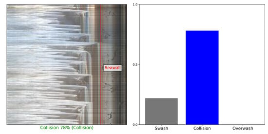
Prediction errors on the test set of Biarritz by the best CNN. The storm impact regime predicted is written under each timestack, and the ground truth is written in parentheses. The probabilities of belonging predicted by the CNN are represented on the right side of each timestack (red = prediction made by CNN, blue = ground truth). The red line in the timestack represents the position of the seawall.
Figure 6.
Prediction errors on the test set of Biarritz by the best CNN. The storm impact regime predicted is written under each timestack, and the ground truth is written in parentheses. The probabilities of belonging predicted by the CNN are represented on the right side of each timestack (red = prediction made by CNN, blue = ground truth). The red line in the timestack represents the position of the seawall.

Table 1.
CNN performances for both sites. Best models are in bold font.
| (a) Biarritz | ||||||
|---|---|---|---|---|---|---|
| CNN | Training Time (min) | Epochs | Time per Epoch (s) | Precision | Recall | -Score |
| Baseline | ||||||
| Custom CNN | 16.1 | 100 | 9.7 | / | 0.333 | 0.328 |
| AlexNet | 17.2 | 100 | 10.3 | / | 0.333 | 0.328 |
| VGG16 | 81.4 | 89 | 54.9 | / | 0.481 | 0.476 |
| Inception v3 | 40.0 | 69 | 34.8 | 0.721 | 0.714 | 0.713 |
| Class weights | ||||||
| Custom CNN | 4.6 | 28 | 9.9 | / | 0.603 | 0.474 |
| AlexNet | 3.8 | 21 | 10.9 | 0.568 | 0.777 | 0.609 |
| VGG16 | 43.4 | 46 | 56.6 | 0.574 | 0.832 | 0.645 |
| Inception v3 | 23.2 | 39 | 35.8 | 0.563 | 0.798 | 0.631 |
| Oversampling | ||||||
| Custom CNN | 10.6 | 26 | 24.6 | 0.642 | 0.880 | 0.718 |
| AlexNet | 11.8 | 27 | 26.1 | 0.716 | 0.885 | 0.777 |
| VGG16 | 69.6 | 28 | 149.1 | 0.783 | 0.851 | 0.813 |
| VGG16 Transfer | 49.9 | 20 | 149.6 | 0.869 | 0.865 | 0.866 |
| Inception v3 | 59.6 | 38 | 94.1 | 0.679 | 0.767 | 0.717 |
| Inception v3 Transfer | 34.5 | 21 | 98.6 | 0.777 | 0.786 | 0.780 |
| (b) Zarautz | ||||||
| CNN | Training Time (Min) | Epochs | Time per Epoch (s) | Precision | Recall | -Score |
| Baseline | ||||||
| Custom CNN | 22.5 | 49 | 27.5 | / | 0.637 | 0.616 |
| AlexNet | 24.0 | 48 | 30.0 | / | 0.628 | 0.616 |
| VGG16 | 202.1 | 72 | 168.4 | / | 0.635 | 0.617 |
| Inception v3 | 108.7 | 64 | 101.9 | / | 0.630 | 0.614 |
| Class weights | ||||||
| Custom CNN | 11.6 | 26 | 26.7 | 0.666 | 0.846 | 0.720 |
| AlexNet | 22.7 | 45 | 30.3 | 0.671 | 0.817 | 0.716 |
| VGG16 | 81.9 | 30 | 163.7 | 0.680 | 0.844 | 0.732 |
| Inception v3 | 89.3 | 53 | 101.1 | 0.654 | 0.838 | 0.710 |
| Oversampling | ||||||
| Custom CNN | 38.7 | 36 | 64.5 | 0.769 | 0.804 | 0.783 |
| AlexNet | 22.6 | 19 | 71.3 | 0.756 | 0.797 | 0.775 |
| VGG16 | 146.6 | 22 | 399.8 | 0.775 | 0.812 | 0.792 |
| VGG16 Transfer | 86.5 | 13 | 399.1 | 0.897 | 0.834 | 0.858 |
| Inception v3 | 97.7 | 24 | 244.2 | 0.777 | 0.801 | 0.784 |
| Inception v3 Transfer | 65.3 | 16 | 245.0 | 0.869 | 0.835 | 0.849 |
Table 2.
Confusion matrices obtained by the best models for both sites.
| (a) Biarritz (best model: OV VGG16 Transfer) | ||||
|---|---|---|---|---|
| Predicted | ||||
| Swash | Collision | Overwash | ||
| Observed | Swash | 1576 | 7 | 0 |
| Collision | 4 | 34 | 2 | |
| Overwash | 1 | 2 | 9 | |
| (b) Zarautz (best model: OV VGG16 Transfer) | ||||
| Predicted | ||||
| Swash | Collision | Overwash | ||
| Observed | Swash | 4265 | 40 | 0 |
| Collision | 13 | 617 | 8 | |
| Overwash | 0 | 25 | 30 | |
Table 3.
Classification results after correcting the misclassification in the test and validation sets.
Table 3.
Classification results after correcting the misclassification in the test and validation sets.
| CNN | Time (min) | Epochs | Time per Epoch (s) | Precision | Recall | F1 Score |
|---|---|---|---|---|---|---|
| Biarritz | ||||||
| Best model before corr. | 49.9 | 20 | 149.6 | 0.869 | 0.865 | 0.866 |
| Best model after corr. | 60 | 24 | 150 | 0.895 | 0.833 | 0.860 |
| Zarautz | ||||||
| Best model before corr. | 86.5 | 13 | 399.1 | 0.897 | 0.834 | 0.858 |
| Best model after corr. | 88.5 | 13 | 408.5 | 0.917 | 0.859 | 0.883 |
Table 4.
Performances of CNN learning from scratch, pre-trained with ImageNet, or pre-trained with the other site for Biarritz and Zarautz. “OV” stands for oversampling.
Table 4.
Performances of CNN learning from scratch, pre-trained with ImageNet, or pre-trained with the other site for Biarritz and Zarautz. “OV” stands for oversampling.
| CNN | Time (min) | Epochs | Time per Epoch (s) | Precision | Recall | -Score |
|---|---|---|---|---|---|---|
| Biarritz | ||||||
| VGG16 (OV) | 69.6 | 28 | 149.1 | 0.783 | 0.851 | 0.813 |
| VGG16 (OV) Pretraining with ImageNet | 49.9 | 20 | 149.6 | 0.869 | 0.865 | 0.866 |
| VGG16 (OV) Pretraining with Zarautz data | 47 | 19 | 148.4 | 0.826 | 0.832 | 0.823 |
| Zarautz | ||||||
| VGG16 (OV) | 81.9 | 30 | 163.7 | 0.680 | 0.844 | 0.732 |
| VGG16 (OV) Pretraining with ImageNet | 86.5 | 13 | 399.1 | 0.897 | 0.834 | 0.858 |
| VGG16 (OV) Pretraining with Biarritz data | 92 | 14 | 394.2 | 0.909 | 0.867 | 0.885 |
Publisher’s Note: MDPI stays neutral with regard to jurisdictional claims in published maps and institutional affiliations. |
© 2021 by the authors. Licensee MDPI, Basel, Switzerland. This article is an open access article distributed under the terms and conditions of the Creative Commons Attribution (CC BY) license (https://creativecommons.org/licenses/by/4.0/).
Share and Cite
MDPI and ACS Style
Callens, A.; Morichon, D.; Liria, P.; Epelde, I.; Liquet, B. Automatic Creation of Storm Impact Database Based on Video Monitoring and Convolutional Neural Networks. Remote Sens. 2021, 13, 1933. https://doi.org/10.3390/rs13101933
AMA Style
Callens A, Morichon D, Liria P, Epelde I, Liquet B. Automatic Creation of Storm Impact Database Based on Video Monitoring and Convolutional Neural Networks. Remote Sensing. 2021; 13(10):1933. https://doi.org/10.3390/rs13101933
Chicago/Turabian StyleCallens, Aurelien, Denis Morichon, Pedro Liria, Irati Epelde, and Benoit Liquet. 2021. "Automatic Creation of Storm Impact Database Based on Video Monitoring and Convolutional Neural Networks" Remote Sensing 13, no. 10: 1933. https://doi.org/10.3390/rs13101933
Note that from the first issue of 2016, this journal uses article numbers instead of page numbers. See further details here.