
Data Fusion of XRF and Vis-NIR Using Outer Product Analysis, Granger–Ramanathan, and Least Squares for Prediction of Key Soil Attributes


Precision Soil and Crop Engineering Group, Department of Environment, Faculty of Bioscience Engineering, Ghent University, 9000 Ghent, Belgium
*
Author to whom correspondence should be addressed.
Remote Sens. 2021, 13(11), 2023; https://doi.org/10.3390/rs13112023
Submission received: 14 April 2021
/
Revised: 12 May 2021
/
Accepted: 19 May 2021
/
Published: 21 May 2021
(This article belongs to the Special Issue Earth Observation in Support of Sustainable Soils Development)
Abstract
:Visible-near-infrared (vis-NIR) and X-ray fluorescence (XRF) are key technologies becoming pervasive in proximal soil sensing (PSS), whose fusion holds promising potential to improve the estimation accuracy of soil attributes. In this paper, we examine different data fusion methods for the prediction of key soil fertility attributes including pH, organic carbon (OC), magnesium (Mg), and calcium (Ca). To this end, the vis-NIR and XRF spectra of 267 soil samples were collected from nine fields in Belgium, from which the soil samples of six fields were used for calibration of the single-sensor and data fusion models while the validation was performed on the remaining three fields. The first fusion method was the outer product analysis (OPA), for which the outer product (OP) of the two spectra is computed, flattened, and then subjected to partial least squares (PLS) regression model. Two versions of OPA were evaluated: (i) OPA-FS in which the full spectra were used as input; and (ii) OPA-SS in which selected spectral ranges were used as input. In addition, we examined the potential of least squares (LS) and Granger–Ramanathan (GR) analyses for the fusion of the predictions provided by the single-sensor PLS models. Results demonstrate that the prediction performance of the single-sensor PLS models is improved by GR in addition to the LS fusion method for all soil attributes since it accounts for residuals. Resorting to LS, the largest improvements compared to the single-sensor models were obtained, respectively, for Mg (residual prediction deviation (RPD) = 4.08, coefficient of determination (R2) = 0.94, ratio of performance of inter-quantile (RPIQ) = 1.64, root mean square error (RMSE) = 4.57 mg/100 g), OC (RPD = 1.79, R2 = 0.69, RPIQ = 2.82, RMSE = 0.16%), pH (RPD = 1.61, R2 = 0.61, RPIQ = 3.06, RMSE = 0.29), and Ca (RPD = 3.33, R2 = 0.91, RPIQ = 1, RMSE = 207.48 mg/100 g). OPA-FS and OPA-SS outperformed the individual, GR, and LS models for pH only, while OPA-FS was effective in improving the individual sensor models for Mg as well. The results of this study suggest LS as a robust fusion method in improving the prediction accuracy for all the studied soil attributes.
1. Introduction
During recent decades, precision agriculture (PA) has emerged as a solution to increase farming efficiency while taking resource limitations and environmental conservation into account [1]. In PA, several proximal soil sensors—including electrical, mechanical, electromagnetic, electro-chemical, and optical sensors—are exploited in order to have accurate assessment of the farming input requirements of plants (crops) during the cropping season. Spectroscopy is one of the methods that is becoming pervasive in PA due to its potential in evaluating the properties of soils and plants [2,3,4] provided in speedy, cost-effective, and environmentally friendly ways. Reports show that the visible and near-infrared (vis-NIR) spectroscopy is the most promising technique in PA, whose performance in prediction of primary properties is usually better than that of the secondary properties [5,6,7,8]. Another powerful method of PSS is XRF spectrometry, which is extensively used in elemental analysis [9]. Nevertheless, its performance in analyzing low-Z elements—i.e., K, P, calcium (Ca), and magnesium (Mg)—is less promising [10,11]. Since neither vis-NIR nor XRF can measure all required soil properties satisfactorily, the hypothesis of the study was that the fusion of the data of the two sensors can improve the prediction accuracy of selected soil (NIR active and non-active) fertility attributes.
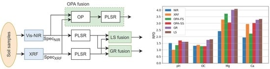
Two possible configurations for fusion of two (or more) kinds of spectrometers, namely, fusion after prediction and prediction after fusion, are shown in Figure 1.
In the former, appropriate prediction models using individual spectrometer data are first developed, whose predicted attributes are fused by resorting to multi-variate linear regression (MLR), referred to also as the Granger–Ramanathan (GR) fusion [12] and model averaging [13]. Adopting this fusion method of XRF and vis-NIR spectrometers in [13] resulted in the improvement of the overall prediction performance between 4% and 44% for different soil attributes. Note that in GR, the weights are computed by implicitly assuming statistical independence among the predictions’ residuals. However, their correlation is considered in the least squares (LS) fusion method [14]. The LS method was evaluated for fusion of vis-NIR and XRF prediction models in [15] using a limited number of soil samples collected from two fields in tropical soils in Brazil, showing LS outperform GR.
In the second fusion method, spectra of different spectrometers are fused first, before the resulting matrix (or vector) is subjected to regression analysis to establish calibration models (Figure 1b). This is referred to as spectral fusion (SF). Common approaches to spectral fusion include spectral concatenation (SC) and outer product analysis (OPA). In SC, different kinds of spectra are first normalized to a comparable range and then concatenated to form a single spectrum. The performance of SC in fusion of vis-NIR and XRF spectra was successful in accuracy improvement of OC and Mg predictions [15,16]. In OPA, the outer product (OP) of a pair of spectra is used as the input to a prediction model. It was shown to be effective in fusion of XRF and vis-NIR spectra for predicting soil chromium content (Cr) by [17]. In addition to SC and OPA, [16] proposed a novel SF method based on convolutional neural network (CNN) for fusion of XRF and vis-NIR spectra. This third SF method structure was successful in improvement of prediction accuracy of soil pH, OC, Mg, and Ca. No previous work was reported on the evaluation of OPA for the assessment of soil pH, OC, Mg, and Ca, in comparison with LS and GR fusion methods.
In this study, the goal was to assess the prediction performance of OPA against LS and GR fusion methods in improvement of the prediction accuracy of four soil attributes including pH, OC, Mg, and Ca using XRF and vis-NIR spectra. One problem with OPA is its demand for high computational resources due to a large matrix produced by OP. Here, we attempted to make OPA computationally more efficient by selecting important spectral and energy ranges of vis-NIR and XRF spectra for each attribute, instead of using full ranges. In LS fusion, the predictions given by the single-sensor PLS models were fused based on the LS method, in which the correlation existing among the residuals of the predictions given by XRF and vis-NIR spectra is considered. Moreover, to evaluate the LS fusion scheme, a noise modification step was introduced whose goal is to make the residual variance of the predictions given by the calibration set the same as that of the validation set. The performance of LS was also compared against GR.
2. Materials and Methods
2.1. Spectroscopy Analysis
In vis-NIR spectroscopy, a light source in the visible and near-infrared range of 300 nm to 2500 nm is illuminated to a soil sample and the resulting diffuse reflectance is detected [18]. Some soil attributes, such as OC, clay, and MC, have direct spectral responses in the NIR range, and hence, they are referred to as primary attributes that can be estimated by the spectrum analysis. It is also possible to estimate some other attributes that are highly correlated with the primary attributes but do not have a direct spectral response in the reflected spectra. In XRF spectroscopy, a certain amount of energy (between 1 KeV and 115 KeV) is radiated by a primary beam taken from an X-ray tube [18,19]. This excites each chemical element to emit secondary spectral lines with wavelengths characteristic of that element and intensities related to its concentration. The intensities are then measured by a detector and can be used to estimate corresponding attributes.
Since spectral properties of soils are highly correlated [20], their dimensionality is reduced prior to applying them to a regression model, including principal component regression (PCR), partial least squares (PLS) regression, and boosted regression trees (BRT), with PLS and BRT being the most popular because of their acceptable performances [21]. In this study, we adopted the PLS regression. Below is a brief description of multivariate statistical methods and data fusion methods adopted in this work.
2.2. Partial Least Squares (PLS) Regression
PLS is one of the popular and widely-used multivariate prediction methods in soil science [22]. It decomposes the matrix of the dependent variables into scores and loadings such that with size of depending on the number of the latent variables. This decomposition is done so that the covariance between scoring T and y is maximized [23].
2.3. Least Squares (LS) Fusion
From the perspective of signal processing, soil properties are considered as unknown deterministic variables (as they are not random). Hence the least squares (LS) method can be adopted in order to estimate them when some observations are available. LS assumes a noisy measurement model with its linear model given by [14]:
where is the ith measurement of the parameter , Hi denotes a linear mapping parameter, is the measurement noise, and m is the number of the available observations. Then, the estimated value is obtained by:
in which z indicates the vector including all samples i = 1, …, m, H is the aggregated matrix of all His, i = 1, …, m, and R indicates the covariance matrix of the samples’ noise. The solution to Equation (2) is given by:
The existence of the inverse of [HTR−1H] amounts to requiring the desired parameter to be observable [24]. Equation (3) clearly implicates a linear relationship between the measurements and the predicted value . However, to calculate the weights in LS according to (3), the covariance matrix R is computed based on the calibration set.
Equation (3) can be rewritten as:
where are the weights obtained via (3). On the other hand, Equation (4) also implicates a popular fusion method known in PA as Granger–Ramanathan (GR) fusion [12] in which the weights are learned through LR (Hereinafter, we avoid referring to this method as LR for consistency. However, we note that GR and LR are basically the same). In GR, the weights are trained in order to minimize the mean squared error, i.e., Equation (2) with R = I. In other words, the measurement noises of sensors—i.e., the residuals—are implicitly assumed to be statistically independent in the solution to GR. Therefore, GR and LS are equivalent in cases with uncorrelated measurement noises. However, as will be discussed later, our experiences show that the noises of the predictions given by XRF and vis-NIR prediction models are often correlated.
2.4. Outer Product Analysis (OPA)
The outer product (OP) of two vectors and computes the product of each element of and all elements of and collects all the products in matrix :
Therefore, includes the cross-correlation values between each sample of and all samples of . Considering the spectra of a soil sample as vectors, the cross-correlation may be advantageous in analysis. In outer product analysis (OPA), the OP matrix is flattened by putting the rows of the matrix along each other. Then, an appropriate modeling method, such as PLS, is used for prediction, as shown in Figure 2 [25].
Accordingly, OPA was initially used in spectroscopy by Barros et al. [26] for relating wavenumbers and wavelengths between vis-NIR and MIR domains. The method was exploited in [27] for studying the effect of temperature on the vis-NIR spectrum of water. Barros et al. [28] showed that the PCs of two vectors, instead of the vectors themselves, can be used for OPA in case the size of the vectors is large and hence to reduce the computational burden. The OPA method was adopted in [25] for fusion of the vis-NIR and MIR spectra where its effectiveness in improvement of the predictions of OC was shown.
In this paper, we examine OPA for fusion of the vis-NIR and XRF spectra. To this end, the procedure shown in Figure 2 is implemented.
2.5. Study Sites and Soil Sampling
In this study, we used in total 267 soil samples from different locations of nine fields in Flanders, Belgium. The soil samples were collected at 10–20 cm soil depth, with an average spatial sampling rate of 3.25 samples/ha during 2018. The fields included Bottelare (5 ha), Thierry (3 ha), Watermachine (6 ha), Beers (12 ha), Kouter (13 ha), Gingelomse (11 ha), Dal (6 ha), Kattestraat (5 ha), and Grootland (21 ha). The information of the study fields is provided in Table 1 with their locations shown in Figure 3. Topographically, the Gingelomse and Bottelare fields had mild undulations, but other fields’ surfaces were rather flat. In addition, there was a high percentage of salt (Ca++) in the soil of Watermachine and Beers located close to the North Sea. Across all fields, a general cropping rotation of maize, potato, sugar beets, and barley/wheat is being performed with an intermittent short-duration cover crop.
2.6. Laboratory Soil Measurement
Each soil sample was reduced to 400 g following standard coning and quartering methods [29]. Each fresh sample was mixed well and its non-soil contents including stones/gravels, grass, and stubble were removed. Then, it was separated into two parts of 200 g each. One part was used for optical measurements in laboratory while the chemical analysis was performed based on the other part. For optical measurements, samples were air-dried for more than two weeks, then they were crushed using an agate mortar and pestle and then they were sieved using a 2 mm stainless steel sieve.
2.6.1. Measurement by X-ray Fluorescence (XRF) Spectrometer
About 2 g of each sieved and dried soil sample was placed on a 30 mm open-ended PANalytical XRF cup with a 44.0 µm Chemplex prolene X-ray film. The film was well set noting that no air bubble exists below it while keeping it unfolded. Just before closing the end caps, we placed a cotton ball so that the soil was held firmly in its position. We used an Oxford XMET-8000 Expert handheld XRF spectrometer (Oxford Instruments, United Kingdom) which was equipped with an Rh X-ray tube (4 W, max. 50 KV, max. 200 µA) and an integrated large-area silicon drift detector (165 eV). Because of safety, the XRF working station was used when operating with the XRF device. The soil samples were put over the scanning window and were scanned in two operating conditions (15 KV at 30 µA; and 45 kV at 30 µA) three times, each time at different positions of the sample. Each scanning took 120 s indicating total scanning time of 360 s for one sample.
2.6.2. Measurement by Visible and Near-Infrared (vis-NIR) Spectrometer
We placed about 50 g of each dried and sieved soil sample into three Petri dishes (diameter = 2 cm and depth = 1 cm). In order to ensure maximum diffuse reflection and increase signal-to-noise ratio [30], each soil sample was gently pressed and leveled using a spatula. We scanned the soil samples using a CompactSpec vis-NIR spectrophotometer (Tec5 Technology for Spectroscopy, Germany) in diffuse reflectance mode, with wavelength range of 305–1700 nm. A 100% reflectance ceramic disc was scanned as the reference for the device calibration every 30 min. Ten spectra per Petri dish were collected, and the resultant 30 spectra per three dishes were averaged in one spectrum per sample.
2.7. Chemical Analysis in Laboratory
The other half part of each soil sample dedicated for the laboratory chemical analysis was kept at 4 °C within a cooling room and then was given to the Soil Survey of Belgium (BDB, Heverlee, Belgium) for chemical analysis of soil OC, pH, Ca, and Mg. OC was obtained using the dry combustion following Dumas principle (ISO 10694; CMA/2/II/A.7; BOC). Before OC measurement, total inorganic carbon compounds were removed by treating the soil samples with hydrochloric (HCl) acid. Soil pH, after shaking and equilibrium for 2 h in mol/l potassium chloride solution (KCl), was measured in the supernatant, using 1:2.5 soil to solution ratio. The available Mg and Ca were determined in ammonium lactate extract with inductively coupled plasma atomic emission spectroscopy (ISO 11885; CMA 2/I/B1). Figure 4 depicts the statistics of the laboratory-measured soil attributes for the soil samples of each field.
2.8. Spectra Pre-Processing
There exist several pre-processing methods for spectroscopy [5,31], since it impacts considerably the prediction accuracy [32]. The best pre-processing scheme is designed based on trial and error and experience and may depend on the desired soil attribute. Accordingly, we examined different pre-processing methods for both XRF and vis-NIR spectra in order to reach the best possible pre-processing steps.
For the vis-NIR spectra, the spectral range between 365 nm and 1600 nm was used since outside this range was noisy and lacked any meaningful information. There was an artifact (spectral jump) around 1045 nm, which is due to the junction of the spectra obtained by two different detectors of different wavelength ranges. This artifact was corrected by subtracting the jump value from the whole reflectance values after 1045 nm [33]. The corrected spectra of 10 randomly chosen samples are shown in Figure 5a. Figure 6a illustrates the pre-processing methods examined for the vis-NIR spectra: (i) R (raw-normalization): applying normalization (removing mean and scaling to unit variance—referred to as standard normal variate (SNV) [34]) on the raw spectra; (ii) S (smoothing-normalization): applying normalization after smoothing the raw spectra by the Savitzky–Golay filter [35], with a window of size 19 and a fitting polynomial of degree 2; and (iii) FD (smoothing-first derivative-normalization): here the first order Savitzky–Golay derivation was normalized.
For the XRF spectra, after several rounds of trial and error, the energy range smaller than 22.4 KeV was selected. The XRF intensities were divided by the live time existing in the report provided by the device in order to correct the counts per second (cps) values. The pre-processing schemes examined for the XRF spectra are depicted in Figure 5b. The first step of pre-processing the XRF spectra was baseline correction which removes existing slope in the spectra. The baseline-corrected spectra were considered as the raw XRF spectra denoted by R which are depicted in Figure 5b. Further treating the spectra by normalizing them with regard to the Compton peak at 20.17 KeV was denoted by C. Smoothing the raw (R) and Compton-normalized (C) spectra using the Savitzky–Golay filter with a window of size 5 and a fitting polynomial of degree 2 was also examined and denoted by RS and CS, respectively. The best pre-processing schemes were specified according to the cross-validation results of the single-sensor models.
Out of the 267 soil samples, 14 samples were detected as outliers using the Mahalanobis distance criterion [36]. We used the soil samples of six fields as the calibration set, while the samples of the remaining three fields were considered for validation. Since the range of each soil attribute was different in different fields (Figure 4), the calibration and validation sets were chosen so that their ranges are comparable in order to reduce the datasets’ impacts on the prediction performances [2,37].
2.9. Single-Sensor Modeling
The PLS model was adopted for predicting the soil attributes using single sensors. To establish the prediction models, first, the most important hyper-parameter of PLS is the number of the latent variables, which was optimized for each soil attribute according to the leave-one-out cross-validation results. Then, the optimal wavelength and energy ranges for vis-NIR and XRF, respectively, were obtained by grid search through all the regression coefficients with the RMSE of the leave-one-out cross-validation as the objective. More specifically, the regression coefficients were sorted first. Then, in each step, the variables with coefficients more than a threshold were used for cross-validation. The set of the variables giving the minimum RMSE was selected and used for calibrating the prediction models. After having the model calibrated, it was validated using the soil samples of the validation fields.
2.10. Fusion Models
Four fusion schemes were evaluated based on OPA, LS, and GR. As discussed in Section 2.3 and Section 2.4, OPA uses the spectral data for fusion while LS and GR fuse the predictions given by single-sensor models. In what follows, fusion of vis-NIR and XRF based on OPA and LS is elaborated. Note that GR is simply a linear regression model based on the outcomes of the vis-NIR and XRF PLS models [12,15]. More details of the method can be found in [15].
2.10.1. OPA-Based Fusion
In order to obtain positive values for OP of the two spectra, they were shifted up such that their minimum values become zero. Two OPA-based prediction models were evaluated:
- OPA-FS in which the full spectral ranges of vis-NIR and XRF were used. In other words, the OP operator was applied on the full spectral ranges.
- OPA-SS in which just the selected spectral ranges of the vis-NIR and XRF spectra, obtained during the calibration of the single-sensor models, were used.
In fact, OPA-FS includes all available information while just the most informative parts of the vis-NIR and XRF spectra, obtained in single sensor modeling (Figure 6), are used in OPA-SS. Since PLS is used in OPA, the same steps shown in Figure 6 were used for evaluation of OPA-FS and OPA-SS models.
2.10.2. LS-Based Fusion
Here, the goal is to improve the estimation accuracy by fusion of the predictions given by the vis-NIR and XRF models as shown in Figure 7. To use LS for fusion, the elements of the covariance matrix, in (3), are computed according to the calibration set by [14]:
where indicates the vector of m given cross-validation predictions given by model , and is the related reference values. Therefore, the covariance matrix is computed and the fused value is obtained by simply using (3) with and . The explicit closed form of (3) is obtained as:
where is the variance of the prediction of sensor , and is the covariance between the predictions of the two sensors.
2.10.3. Noise Modification
To evaluate the performance of the LS-based fusion as well as GR, the predictions given by the single-sensor PLS models are used (e.g., and in Figure 6). In fact, training of the whole system should be performed in two stages: (i) training the PLS models and (ii) training the data fusion scheme. However, those predictions of the PLS models that are based on the calibration set are more precise than the predictions based on the validation sets, as expected. In order to take advantage of all available predictions and not limiting to just the predictions of the validation set at the second stage of training, a noise modification step was applied to the calibration predictions.
We can model the prediction given by the PLS model k as:
where is the prediction residual assumed to be distributed according to the normal distribution. As expected and can be observed in Figure 7, the predictions given by the calibration set have less variance than the validation set. If the variances of the calibration and validation sets are, respectively, denoted by and , a noise should be added to the prediction k of the calibration set. After the noise modification—as shown in Figure 8—the whole available predictions, i.e., both calibration and validation predictions, can be used for training and testing the data fusion schemes.
2.11. Evaluation Criteria
The prediction performance of the single-sensor and fusion models were evaluated in terms of root mean square error (RMSE), ratio of performance to deviation (RPD), coefficient of determination (R2), and ratio of performance to inter-quartile (RPIQ). R2 depicts how much a model performs and better than using just a very well fitted hyperplane. RPD is obtained by dividing the standard deviation of the measurements by RMSE [8]. RPIQ is given by:
in which Q1 and Q3 are the upper bounds of the first and third quartiles of the measurements, respectively. In other words, the range covered by the second and third quartiles is used by RPIQ to estimate the prediction accuracy. This range might represent the spread of the soil attributes’ values better than their standard deviation which is used by RPD [8]. In fact, [38] SD is suitable for normally distributed measurements while the distribution of soil attributes is usually skewed. However, since RPD has been adopted extensively in the literature, we included it as one of the evaluation criteria. The single-sensor and sensor-fusion models were implemented and evaluated using Python and, especially, its scikit-learn package [39].
3. Results and Discussions
In order to have comparable calibration and validation sets, different fields were used for evaluating the prediction models of each soil attribute, as listed in Table 2. Figure 9 illustrates the box plots of the calibration and validation sets used for the prediction models of each soil attribute. As shown, although the selection of the calibration and validation fields was carefully made, large differences in the ranges of the calibration and validation set can still be observed, which will have negative influence on the prediction performance of the prediction models. The issue becomes worse if the range of the calibration set is smaller than that of the validation set [2,37], where part of the concentration range of the validation set will not be accounted for in the calibration models.
The optimal number of the latent variables used in the PLS models is listed in Table 3, showing a low number of latent variables used in all modeling schemes, reflecting robustness. The best pre-processing schemes were obtained according to the PLS modeling of vis-NIR and XRF resulted in the optimal number of latent variables. Comparing individual vis-NIR models against corresponding XRF models indicates that the latter groups of models were better just for Ca. For vis-NIR, the cross-validation results—shown in Figure 10 (for brevity in the figures, NIR denotes vis_NIR)—indicate that SNV alone was the best pre-processing scheme for pH and OC while SN and FD were the best pre-processing methods for Mg and Ca, respectively. In case of XRF, Compton normalization and in combination with smoothing (i.e., CS) improved the prediction accuracy of OC. For pH and Ca, just the baseline correction (i.e., R) was sufficient and more smoothing improved the prediction performance of Mg. It is worth noting that the inelastic scattering due to the Rh tube of the XRF device may result in misleading information that degrades the prediction performance. To neutralize this performance degradation, the XRF spectra are suggested to be normalized to the Compton peaks (Yılmaz and Boydaş, 2018). However, this was effective for OC only in the current work (Figure 10).
After optimizing the number of the latent variables according to the cross-validation analysis and selecting the best pre-processing schemes, the optimal wavelength and energy ranges were obtained as shown in Figure 11. Variable selection results in more effective and simpler prediction models which give better accuracies [40], as discussed in Section 3.1. The optimal spectral and energy ranges were used for validating the single-sensor models and comparing their performance with each other as well as the data fusion methods. The validation results are illustrated in Figure 12. In what follows, the validation results are explored in detail.
3.1. Assessment of Vis-NIR and XRF Individual Models
Comparing the validation results in Figure 12 with the best cross-validation results in Figure 10 shows that similar performances were obtained which indicates the robustness of the single-sensor models. The validation accuracies for OC and Mg from XRF were even improved compared to the cross-validation results which might be due to using the optimal energy ranges used in validation. In fact, wavelength and energy selection simplifies the prediction models by reducing the number of their parameters (weights). Therefore, the models will be trained more accurately using the same training dataset [40]. Moreover, just the informative parts of the spectra will be used while the non-contributing parts will be omitted. It is worth emphasizing that these results are independent validation results, as the models produced using data of six fields were validated using data of the remaining three fields that were not used in model calibration.
As shown in Figure 12, the predictions given by the vis-NIR spectra outperformed the XRF for pH only. Though XRF outperformed vis-NIR for Ca (RPD = 2.95) and Mg (RPD = 3.27), the performance of vis-NIR was also acceptable with RPD = 1.94 and RPD = 2.42 for Ca and Mg, respectively. Similar performance was reported by [41] for Ca based on vis-NIR modeling with a backpropagation neural network with latent variables derived from a PLS analysis used as input. The more accurate Ca and Mg predictions of XRF are attributed to the high intensity of fluorescence emission from Ca, compared to other elements [42,43]. It is interesting that the optimal energy range for Ca includes its related kα line at 3.69 KeV (Figure 11b). It is well-known that there is a positive correlation between XRF fluorescence intensity and the atomic mass of elements [44]. More specifically, the higher the atomic mass, the higher is the XRF intensity. That is why the XRF technology is very popular in the elemental analysis of heavy metals in soil environment [45] than the elements having lower atomic mass [11]. The validation results in this study coincide with the findings reported earlier [11], confirming that XRF is limited in prediction of light soil elements, such as those considered in the present work. Indeed, vis-NIR was proven in this work to be a better sensing technique than XRF for quantifying these light soil attributes.
The validation results implicate a better accuracy for the prediction of pH, OC, and Ca compared to those reported by [16], which might be due to more efficient pre-processing steps and using the optimal spectral and energy ranges in the current work. Note that the Mg accuracies obtained in this study were acceptable with RPD more than 2.3 for both vis-NIR and XRF models. The current study illustrates that selection of most significant optical bands is the way forward to improve the prediction accuracy of the studied soil parameters using vis-NIR and XRF spectroscopy.
3.2. Assessment of OPA-Based Fusion Methods
Figure 13 shows the OP result of the vis-NIR spectrum of a soil sample and its corresponding XRF spectrum. As seen, the OP is higher where there are significant changes in the spectra. Accordingly, OPA-PLS model accuracy is expected to be higher for the soil attributes, for which those significant changes are jointly used in their single-sensor predictions. In other words, if the optimal wavelength and energy ranges include significant changes in both vis-NIR reflectance and XRF intensity spectra, OPA is expected to improve the accuracy. Specifically, the optimal energy ranges of OC do not include any significant changes (e.g., around the XRF emission lines at 5.4, 6.08, 14.78, 18.91, and 19.21 KeV) which means their OP will not be informative. Hence, OPA-FS and OPA-SS failed in fusion of the two kinds of the spectra in predicting OC (Figure 12). However, the prediction accuracy of Mg was improved appropriately by OPA-FS, compared to the single-sensor models. In fact, OPA-FS outperformed OPA-SS in the prediction of Mg (RPD = 3.72, RPIQ = 1.51, RMSE = 4.98 mg/100 g). Comparing with the CNN-based spectral fusion proposed by [16], OPA was inferior in both accuracy and computational complexity, since it produces a high-dimensional matrix, to be used as input.
3.3. Assessment of LS
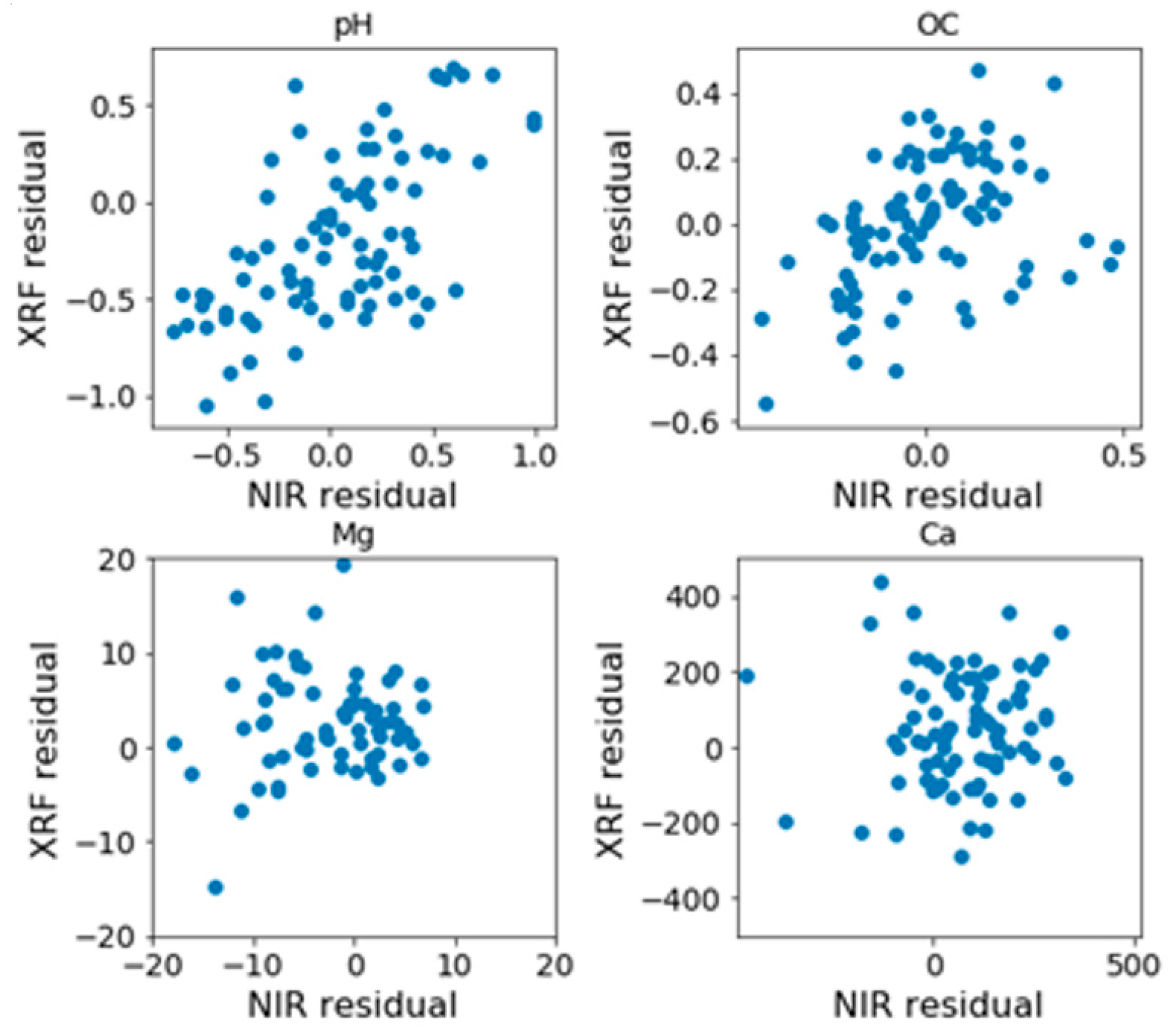
As discussed in Section 2.10.2, LS considers the correlation between the residuals of the predictions given by the PLS models. Figure 14 depicts that the prediction residuals of vis-NIR and XRF are correlated with their Pearson correlation coefficient listed in Table 4. Therefore, it is expected that LS performs at least as well as GR for cases with correlated noises. In fact, the sensors’ noises (residuals) are assumed to be statistically independent in most scenarios [46,47]. While this is true for different sensors, this is not the case in spectroscopy where the predictions are made based on spectra input (Figure 1a). Different kinds of spectra may share the same interference impact from the soil samples (e.g., due to existence of some other chemicals within the soil sample). This will result in correlated prediction residuals that should be taken into account when data are fused. The more correlation exists among residuals, the more improvement is expected from LS compared to GR. Similar comparative results were also observed by [15] for Brazilian soils. However, the results of this study are more credible since they were obtained after noise modification. Moreover, more samples were used and the fusion methods were evaluated in a non-spiking strategy using independent samples collected from three fields (validation set) that were not used in the calibration. In other words, no samples of the three validation fields were used in the calibration.
It is worth mentioning that redundancy should be noted when data fusion is performed. In other words, each piece of information should be counted once, and the fusion method should be able to distinguish the redundant information, while taking advantage of synergy in available data. This is accomplished in LS by considering the correlation among the prediction residuals. The more accurate the correlation is computed, the more improvement in prediction accuracy will be achieved. In this study, LS was shown to be a robust fusion method in terms of improving the prediction accuracy compared to the single-sensor models. This indicates that considering the correlation existing among the residuals improves the accuracy compared to training the linear regression coefficient with an objective function ignoring the correlation [48]. LS improved the single-sensor prediction accuracies for all four attributes and stood out as the best fusion method, except for Mg where OPA-FS accuracy was better.
4. Conclusions
In this paper, the individual performance of vis-NIR and XRF spectroscopy and their fusion were evaluated in an analysis of soil pH, OC, Mg, and Ca using 267 soil samples from nine fields in Belgium. Partial least squares regression (PLS) with different pre-processing schemes was examined for modeling individual sensor data with and without variable selection. The validation results reveal that the variable selection makes the single-sensor calibration models more efficient by reducing the number of the models’ parameters, resulting in improving their prediction accuracies.
For data fusion, two configurations were discussed, namely, prediction after fusion and fusion after prediction. For the former case, two spectral fusion methods based on outer product analysis (OPA) were examined: (i) OPA-FS which uses the outer product (OP) of the full spectral ranges of the vis-NIR and XRF spectra; and (ii) OPA-SS which considers the optimal spectral ranges of the two spectral kinds as input. OPA-FS was generally more effective than OPA-SS as it improved the predictions for pH and Mg with their ranges consisting of significant spectral changes. For the second fusion configuration, least squares (LS)-based fusion approach was elaborated and examined. Results reveal that, in general, the fusion models outperformed individual sensor models for all investigated soil properties. It was observed that the residuals of the predictions given by the single-sensor models are correlated while this correlation is ignored in the objective function of the more common Granger–Ramanathan (GR) fusion method. In LS, the correlation among the residuals of the predictions is considered. We demonstrated that LS performance is at least the same as the GR fusion method. In order to correctly evaluate the fusion schemes using all available samples, a noise modification step was introduced whose goal was to modify the noise variance given by the calibration set according to that of the validation set.
Overall, the validation results of this study suggested LS as the most robust fusion method in terms of reaching high accuracy across all key attributes. By LS, the following independent prediction accuracies were achieved: RPD = 4.08, R2 = 0.94, RPIQ = 1.64, RMSE = 4.57 mg/100 g for Mg; RPD = 3.33, R2 = 0.91, RPIQ = 1, RMSE = 207.48 mg/100 g for Ca; RPD = 1.61, R2 = 0.61, RPIQ = 3.06, RMSE = 0.29 for pH; and RPD = 1.79, R2 = 0.69, RPIQ = 2.82, RMSE = 0.16% for OC. However, OPA-FS fusion method outperformed all individual sensor models and fusion models including LS just for Mg.
Examining the LS method for fusion of other types of spectra (e.g., vis-NIR with MIR and XRF) and also specifying the informative wavelength ranges for each attribute and using just those ranges in prediction modeling and fusion can be considered as interesting future topics.
Author Contributions
Conceptualization, S.H.J. and A.M.M.; methodology, S.H.J.; software, S.H.J.; validation, S.H.J. and A.M.M.; formal analysis, S.H.J.; investigation, S.H.J. and A.M.M.; resources, S.H.J. and A.M.M.; data curation, S.H.J.; writing—original draft preparation, S.H.J.; writing—review and editing, A.M.M.; visualization, S.H.J.; supervision, A.M.M.; project administration, A.M.M.; funding acquisition, A.M.M. Both authors have read and agreed to the published version of the manuscript.
Funding
This research was funded by Research Foundation Flanders (FWO), grant number G0F9216N.
Institutional Review Board Statement
Not applicable.
Informed Consent Statement
Not applicable.
Data Availability Statement
The data presented in this study are available on request from the corresponding author. The data are not publicly available since they are considered as confidential for the Precision Scoring group at Ghent University for the moment.
Conflicts of Interest
The authors declare no conflict of interest.
References
- Mouazen, A.M.; Maleki, M.R.; De Baerdemaeker, J.; Ramon, H. Monitoring. In Agricultural Internet of Things and Decision Support for Precision Smart Farming; Castrignanò, A., Buttafuoco, G., Khosla, R., Mouazen, A., Moshou, D., Naud, O., Eds.; Academic Press: Cambridge, MA, USA, 2019; pp. 36–138. [Google Scholar]
- Stenberg, B.; Rossel, R.A.V.; Mouazen, A.M.; Wetterlind, J. Chapter Five—Visible and Near Infrared Spectroscopy. In Soil Science; Sparks, D.L., Ed.; Academic Press: Cambridge, MA, USA, 2010; pp. 163–215. [Google Scholar]
- Guzmán, J.A.Q.; Rivard, B.; Sánchez-Azofeifa, G.A. Discrimination of liana and tree leaves from a Neotropical Dry Forest using visible-near infrared and longwave infrared reflectance spectra. Remote Sens. Environ. 2018, 219, 135–144. [Google Scholar] [CrossRef]
- Ben-Dor, E.; Banin, A. Visible and near-infrared (0.4–1.1 μm) analysis of arid and semiarid soils. Remote Sens. Environ. 1994, 48, 261–274. [Google Scholar] [CrossRef]
- Mouazen, A.; De Baerdemaeker, J.; Ramon, H. Effect of wavelength range on the measurement accuracy of some selected soil constituents using visual-near infrared spectroscopy. J. Near Infrared Spectrosc. 2006, 14, 189–199. [Google Scholar] [CrossRef]
- Marín-González, O.; Kuang, B.; Quraishi, M.Z.; Munóz-García, M. Ángel; Mouazen, A.M. Online measurement of soil properties without direct spectral response in near infrared spectral range. Soil Tillage Res. 2013, 132, 21–29. [Google Scholar] [CrossRef] [Green Version]
- Munnaf, M.A.; Nawar, S.; Mouazen, A.M. Estimation of secondary soil properties by fusion of laboratory and online measured Vis–NIR spectra. Remote Sens. 2019, 11, 2819. [Google Scholar] [CrossRef] [Green Version]
- Chang, C.-W.; Laird, D.A.; Mausbach, M.J.; Hurburgh, C.R. Near-infrared reflectance spectroscopy-principal components regression analyses of soil properties. Soil Sci. Soc. Am. J. 2001, 65, 480–490. [Google Scholar] [CrossRef] [Green Version]
- Wang, D.; Chakraborty, S.; Weindorf, D.C.; Li, B.; Sharma, A.; Paul, S.; Ali, N. Synthesized use of VisNIR DRS and PXRF for soil characterization: Total carbon and total nitrogen. Geoderma 2015, 243–244, 157–167. [Google Scholar] [CrossRef]
- Kaniu, M.; Angeyo, K.; Mwala, A.; Mwangi, F. Energy dispersive X-ray fluorescence and scattering assessment of soil quality via partial least squares and artificial neural networks analytical modeling approaches. Talanta 2012, 98, 236–240. [Google Scholar] [CrossRef] [PubMed]
- Nawar, S.; Delbecque, N.; Declercq, Y.; De Smedt, P.; Finke, P.; Verdoodt, A.; Van Meirvenne, M.; Mouazen, A.M. Can spectral analyses improve measurement of key soil fertility parameters with X-ray fluorescence spectrometry? Geoderma 2019, 350, 29–39. [Google Scholar] [CrossRef]
- Granger, C.W.J.; Ramanathan, R. Improved methods of combining forecasts. J. Forecast. 1984, 3, 197–204. [Google Scholar] [CrossRef]
- O’Rourke, S.; Stockmann, U.; Holden, N.; McBratney, A.; Minasny, B. An assessment of model averaging to improve predictive power of portable vis-NIR and XRF for the determination of agronomic soil properties. Geoderma 2016, 279, 31–44. [Google Scholar] [CrossRef]
- Papoulis, A.; Pillai, S.U. Probability, Random Variables and Stochastic Processes, 4th ed.; McGraw-Hill: New York, NY, USA, 2002. [Google Scholar]
- Tavares, T.R.; Molin, J.P.; Javadi, S.H.; De Carvalho, H.W.P.; Mouazen, A.M. Combined use of vis-NIR and XRF sensors for tropical soil fertility analysis: Assessing different data fusion approaches. Sensors 2020, 21, 148. [Google Scholar] [CrossRef]
- Javadi, S.H.; Munnaf, M.A.; Mouazen, A.M. Fusion of Vis-NIR and XRF spectra for estimation of key soil attributes. Geoderma 2021, 385, 114851. [Google Scholar] [CrossRef]
- Xu, D.; Chen, S.; Rossel, R.V.; Biswas, A.; Li, S.; Zhou, Y.; Shi, Z. X-ray fluorescence and visible near infrared sensor fusion for predicting soil chromium content. Geoderma 2019, 352, 61–69. [Google Scholar] [CrossRef]
- Zude, M. Optical Monitoring of Fresh and Processed Agricultural Crops; CRC Press: Boca Raton, FL, USA, 2009. [Google Scholar]
- Tavares, T.R.; Molin, J.P.; Nunes, L.C.; Alves, E.E.N.; Melquiades, F.L.; De Carvalho, H.W.P.; Mouazen, A.M. Effect of X-Ray Tube Configuration on Measurement of Key Soil Fertility Attributes with XRF. Remote. Sens. 2020, 12, 963. [Google Scholar] [CrossRef] [Green Version]
- Mouazen, A.M.; Kuang, B. On-line visible and near infrared spectroscopy for in-field phosphorous management. Soil Tillage Res. 2016, 155, 471–477. [Google Scholar] [CrossRef]
- Gholizadeh, A.; Borůvka, L.; Saberioon, M.; Vašát, R. A memory-based learning approach as compared to other data mining algorithms for the prediction of soil texture using diffuse reflectance spectra. Remote Sens. 2016, 8, 341. [Google Scholar] [CrossRef] [Green Version]
- Nawar, S.; Cipullo, S.; Douglas, R.K.; Coulon, F.; Mouazen, A.M. The applicability of spectroscopy methods for estimating potentially toxic elements in soils: State-of-the-art and future trends. Appl. Spectrosc. Rev. 2020, 55, 525–557. [Google Scholar] [CrossRef]
- Casa, R.; Castaldi, F.; Pascucci, S.; Basso, B.; Pignatti, S. Geophysical and hyperspectral data fusion techniques for in-field estimation of soil properties. Vadose Zone J. 2013, 12, 201. [Google Scholar] [CrossRef]
- Bar-Shalom, Y.; Li, X.-R.; Kirubarajan, T. Estimation with Applications to Tracking and Navigation; John Wiley & Sons, Inc.: New York, NY, USA, 2001. [Google Scholar]
- Terra, F.S.; Rossel, R.A.V.; Demattê, J.A. Spectral fusion by Outer Product Analysis (OPA) to improve predictions of soil organic C. Geoderma 2019, 335, 35–46. [Google Scholar] [CrossRef]
- Barros, A.S.; Safar, M.; Devaux, M.F.; Robert, P.; Bertrand, D.; Rutledge, D.N. Relations between Mid-Infrared and Near-Infrared Spectra Detected by Analysis of Variance of an Intervariable Data Matrix. Appl. Spectrosc. 1997, 51, 1384–1393. [Google Scholar] [CrossRef]
- Jaillais, B.; Pinto, R.; Barros, A.; Rutledge, D. Outer-product analysis (OPA) using PCA to study the influence of temperature on NIR spectra of water. Vib. Spectrosc. 2005, 39, 50–58. [Google Scholar] [CrossRef]
- Barros, A.; Pinto, R.; Bouveresse, D.J.-R.; Rutledge, D. Principal component transform—Outer product analysis in the PCA context. Chemom. Intell. Lab. Syst. 2008, 93, 43–48. [Google Scholar] [CrossRef]
- Mukhopadhyay, S.; Maiti, S.K. Techniques for Quantative Evaluation of Mine Site Reclamation Success: Case Study; Elsevier: Amsterdam, The Netherlands, 2018; pp. 415–438. [Google Scholar]
- Mouazen, A.; Saeys, W.; Xing, J.; De Baerdemaeker, J.; Ramon, H. Near Infrared Spectroscopy for Agricultural Materials: An Instrument Comparison. J. Near Infrared Spectrosc. 2005, 13, 87–97. [Google Scholar] [CrossRef]
- Moura-Bueno, J.M.; Dalmolin, R.S.D.; Caten, A.T.; Dotto, A.C.; Demattê, J.A. Stratification of a local VIS-NIR-SWIR spectral library by homogeneity criteria yields more accurate soil organic carbon predictions. Geoderma 2019, 337, 565–581. [Google Scholar] [CrossRef]
- Rinnan, Å.; Berg, F.V.D.; Engelsen, S.B. Review of the most common pre-processing techniques for near-infrared spectra. TrAC Trends Anal. Chem. 2009, 28, 1201–1222. [Google Scholar] [CrossRef]
- Mouazen, A.; Maleki, M.; Cockx, L.; Van Meirvenne, M.; Van Holm, L.; Merckx, R.; De Baerdemaeker, J.; Ramon, H. Optimum three-point linkage set up for improving the quality of soil spectra and the accuracy of soil phosphorus measured using an on-line visible and near infrared sensor. Soil Tillage Res. 2009, 103, 144–152. [Google Scholar] [CrossRef] [Green Version]
- Barnes, R.J.; Dhanoa, M.S.; Lister, S.J. Standard normal variate transformation and de-trending of near-infrared diffuse reflectance spectra. Appl. Spectrosc. 1989, 43, 772–777. [Google Scholar] [CrossRef]
- Savitzky, A.; Golay, M.J.E. Smoothing and differentiation of data by simplified least squares procedures. Anal. Chem. 1964, 36, 1627–1639. [Google Scholar] [CrossRef]
- De Maesschalck, R.; Jouan-Rimbaud, D.; Massart, D.L. The Mahalanobis distance. Chemom. Intell. Lab. Syst. 2000, 50, 1–18. [Google Scholar] [CrossRef]
- Nawar, S.; Mouazen, A.M. Optimal sample selection for measurement of soil organic carbon using on-line vis-NIR spectroscopy. Comput. Electron. Agric. 2018, 151, 469–477. [Google Scholar] [CrossRef]
- Bellon-Maurel, V.; Fernandez-Ahumada, E.; Palagos, B.; Roger, J.-M.; McBratney, A. Critical review of chemometric indicators commonly used for assessing the quality of the prediction of soil attributes by NIR spectroscopy. TrAC Trends Anal. Chem. 2010, 29, 1073–1081. [Google Scholar] [CrossRef]
- Pedregosa, F.; Varoquaux, G.; Gramfort, A.; Michel, V.; Thirion, B.; Grisel, O.; Duchesnay, E.; Vanderplas, J.; Passos, A.; Cournapeau, D.; et al. Scikit-learn: Machine learning in python. J. Mach. Learn. Res. 2011, 12, 2825–2830. [Google Scholar]
- Hu, L.; Yin, C.; Ma, S.; Liu, Z. Rapid detection of three quality parameters and classification of wine based on Vis-NIR spectroscopy with wavelength selection by ACO and CARS algorithms. Spectrochim. Acta Part A Mol. Biomol. Spectrosc. 2018, 205, 574–581. [Google Scholar] [CrossRef] [PubMed]
- Mouazen, A.; Kuang, B.; De Baerdemaeker, J.; Ramon, H. Comparison among principal component, partial least squares and back propagation neural network analyses for accuracy of measurement of selected soil properties with visible and near infrared spectroscopy. Geoderma 2010, 158, 23–31. [Google Scholar] [CrossRef]
- Teixeira, A.F.D.S.; Weindorf, D.C.; Silva, S.H.G.; Guilherme, L.R.G.; Curi, N. Portable X-ray fluorescence (pXRF) spectrometry applied to the prediction of chemical attributes in Inceptisols under different land uses. Ciência e Agrotecnologia 2018, 42, 501–512. [Google Scholar] [CrossRef]
- Silva, S.H.G.; Teixeira, A.F.D.S.; De Menezes, M.D.; Guilherme, L.R.G.; Moreira, F.M.D.S.; Curi, N. Multiple linear regression and random forest to predict and map soil properties using data from portable X-ray fluorescence spectrometer (pXRF). Ciência e Agrotecnologia 2017, 41, 648–664. [Google Scholar] [CrossRef]
- Russ, J.C. Fundamentals of Energy Dispersive X-ray Analysis. In Fundamentals of Energy Dispersive X-ray Analysis; Elsevier: Amsterdam, The Netherlands, 1984; pp. 208–219. [Google Scholar]
- Soodan, R.K.; Pakade, Y.B.; Nagpal, A.; Katnoria, J.K. Analytical techniques for estimation of heavy metals in soil ecosystem: A tabulated review. Talanta 2014, 125, 405–410. [Google Scholar] [CrossRef] [PubMed]
- Javadi, S.H. Detection over sensor networks: A tutorial. IEEE Aerosp. Electron. Syst. Mag. 2016, 31, 2–18. [Google Scholar] [CrossRef]
- Javadi, S.H.; Farina, A. Radar networks: A review of features and challenges. Inf. Fusion 2020, 61, 48–55. [Google Scholar] [CrossRef] [Green Version]
- Chang, N.-B.; Bai, K. Multisensor Data Fusion and Machine Learning for Environmental Remote Sensing; CRC Press: Boca Raton, FL, USA, 2018. [Google Scholar]
Figure 1.
Two possible configurations for data fusion in spectroscopy: (a) fusion after prediction and (b) prediction after fusion (spectral fusion).
Figure 1.
Two possible configurations for data fusion in spectroscopy: (a) fusion after prediction and (b) prediction after fusion (spectral fusion).

Figure 2.
The outer product analysis (OPA) [25] method in fusion of spectral data.
Figure 2.
The outer product analysis (OPA) [25] method in fusion of spectral data.

Figure 3.
Belgium map with the geographic locations of the studied fields identified.

Figure 4.
The box plot of the laboratory-measured soil organic carbon (OC), pH, magnesium (Mg), and calcium (Ca) per each field including Grootland (Gr), Beers (Be), Kouter (Ko), Bottelare (Bo), Dal (Da), Kattestraat (Ka), Gingelomse (Gi), Watermachine (Wa), and Thierry (Th). Since the ranges of Ca in Grootland and Beers were much larger than those of other fields, they are depicted separately.
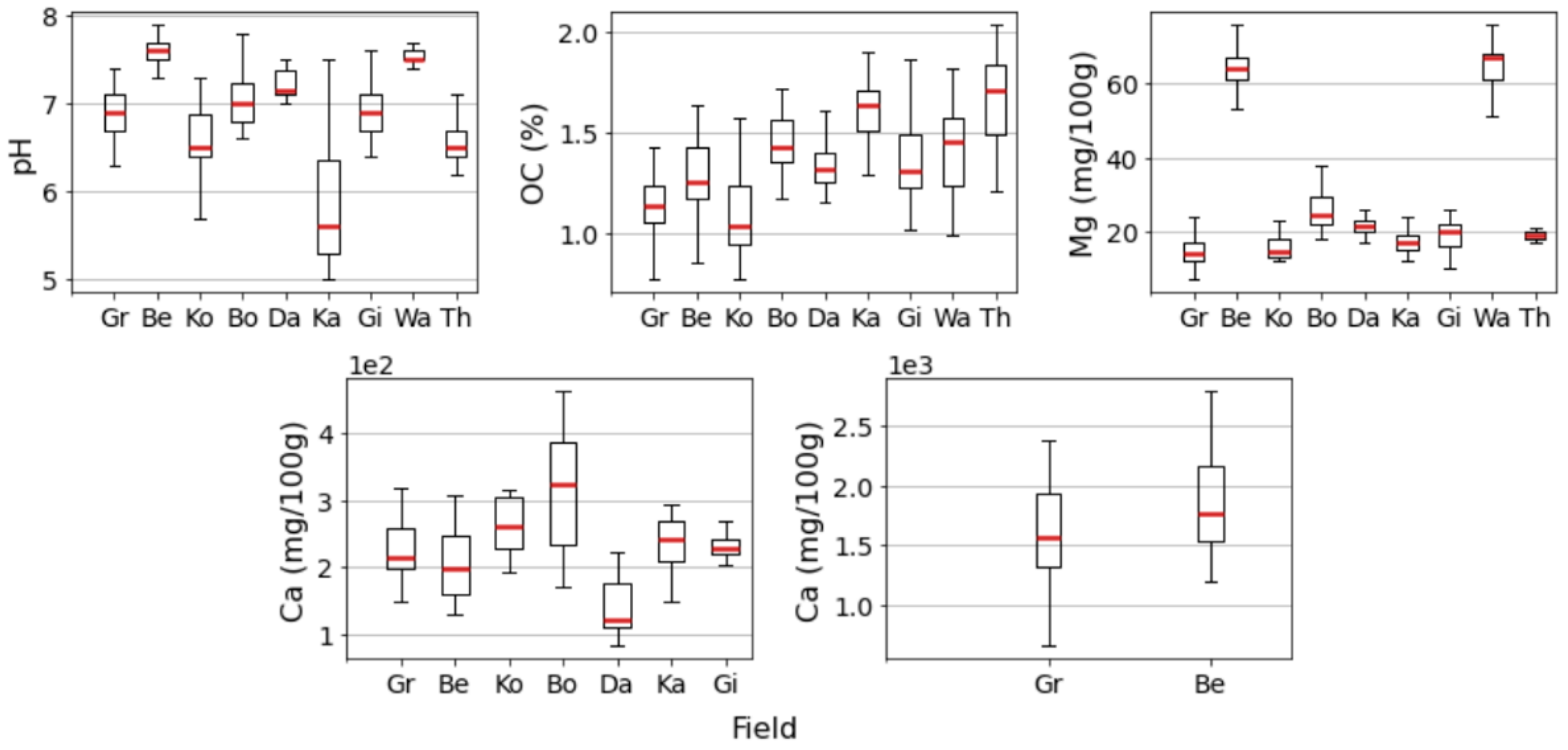
Figure 5.
The visible-near-infrared (vis-NIR) spectra (a) and X-ray florescence (XRF) spectra (b) of 10 soil samples chosen randomly from 267 soil samples used after removal of outliers.
Figure 5.
The visible-near-infrared (vis-NIR) spectra (a) and X-ray florescence (XRF) spectra (b) of 10 soil samples chosen randomly from 267 soil samples used after removal of outliers.
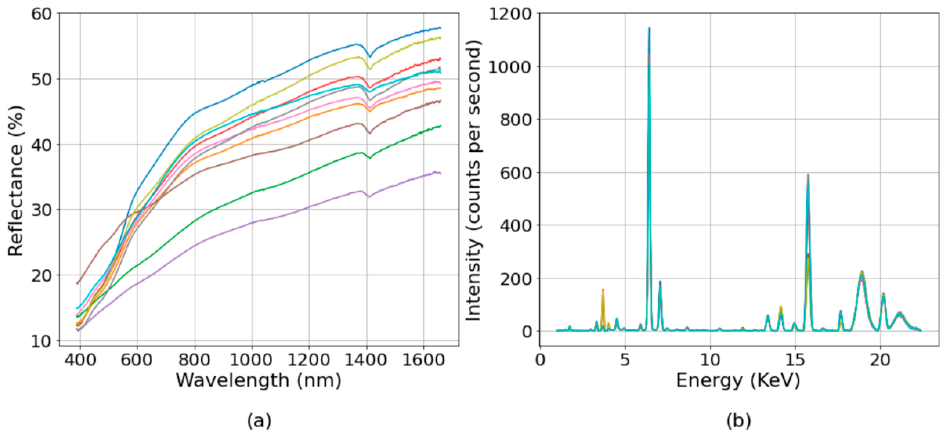
Figure 6.
(a) The pre-processing steps for the visible-near-infrared (vis-NIR) spectra including raw-normalization (R), smoothing using Savitzky–Golay filter (SGF) and then normalization (S), and first derivative (FD) and then normalization (FD). Normalization is based on standard normal variate (SNV). (b) The pre-processing steps for the X-ray fluorescence (XRF) spectra including raw (R), Compton-normalized (C), Compton-normalized-smoothed (CS), and raw-smoothed (RS).
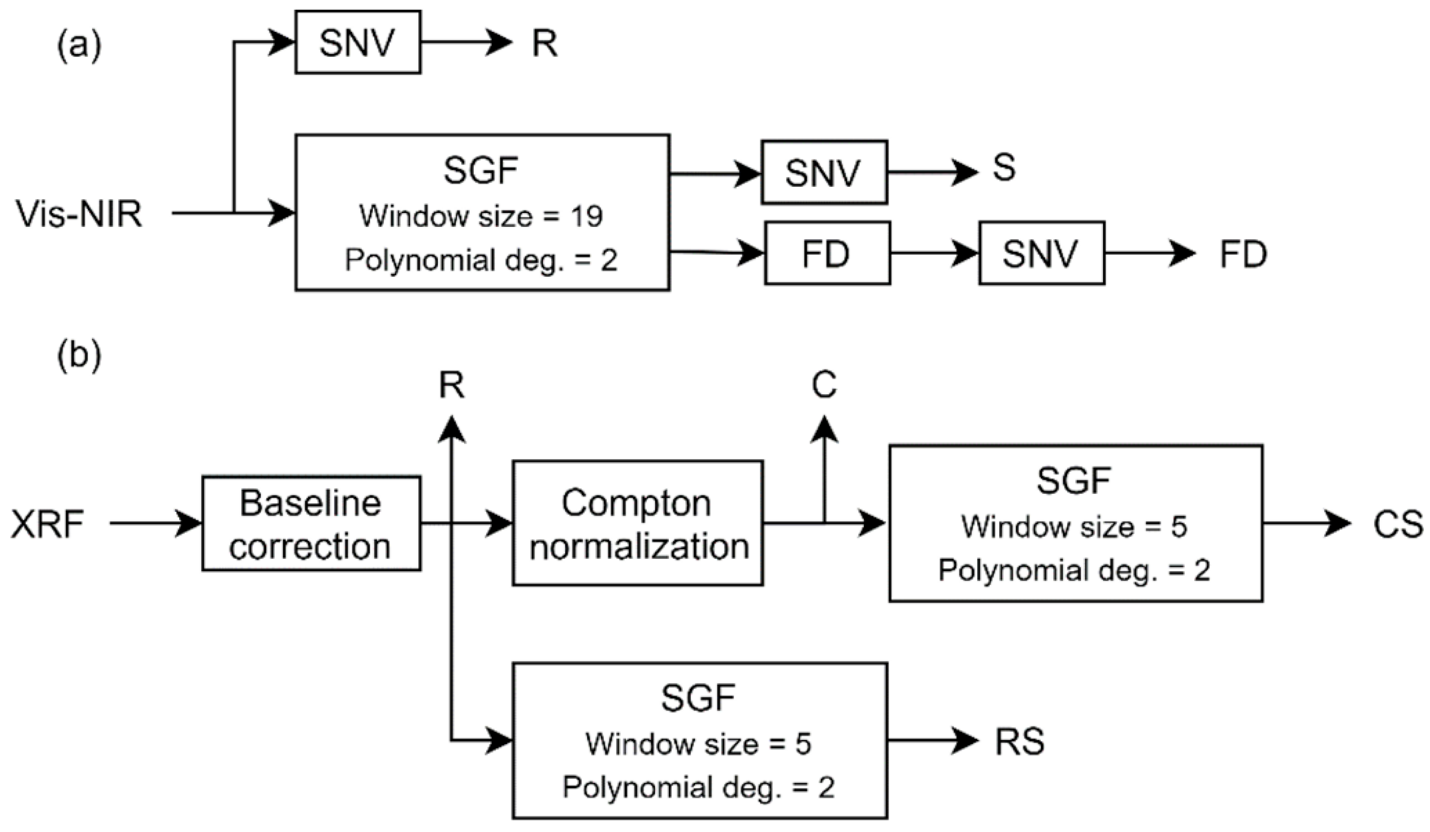
Figure 7.
Fusion of the predictions given by the visible-near-infrared (vis-NIR) and X-ray fluorescence (XRF) spectra.
Figure 7.
Fusion of the predictions given by the visible-near-infrared (vis-NIR) and X-ray fluorescence (XRF) spectra.

Figure 8.
Modifying the residuals (noises) of the calibration predictions given by the partial least squares (PLS) models.
Figure 8.
Modifying the residuals (noises) of the calibration predictions given by the partial least squares (PLS) models.
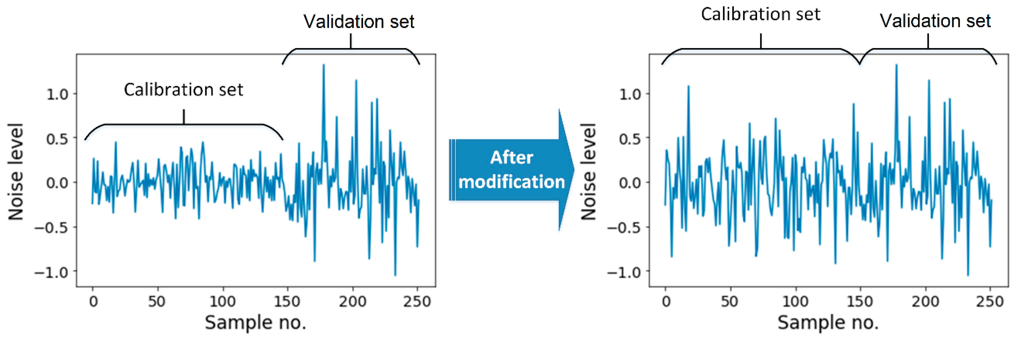
Figure 9.
Box plots of the soil attributes and the calibration and validation datasets for pH, organic carbon (OC), magnesium (Mg), and calcium (Ca).
Figure 9.
Box plots of the soil attributes and the calibration and validation datasets for pH, organic carbon (OC), magnesium (Mg), and calcium (Ca).

Figure 10.
The prediction performance of partial least squares (PLS) in cross-validation modeling of visible-near-infrared (NIR) and X-ray fluorescent (XRF) spectra, under different pre-processing strategies for NIR: R: raw spectra normalized, S: smoothed normalized, FD: first derivative normalized; and for XRF: C: Compton-normalized, RS: raw spectra smoothed, CS: Compton-normalized and smoothed. RMSE: root mean square error; RPD: ratio of performance to deviation; R2: coefficient of determination; RPIQ: ratio of performance to inter-quartile.
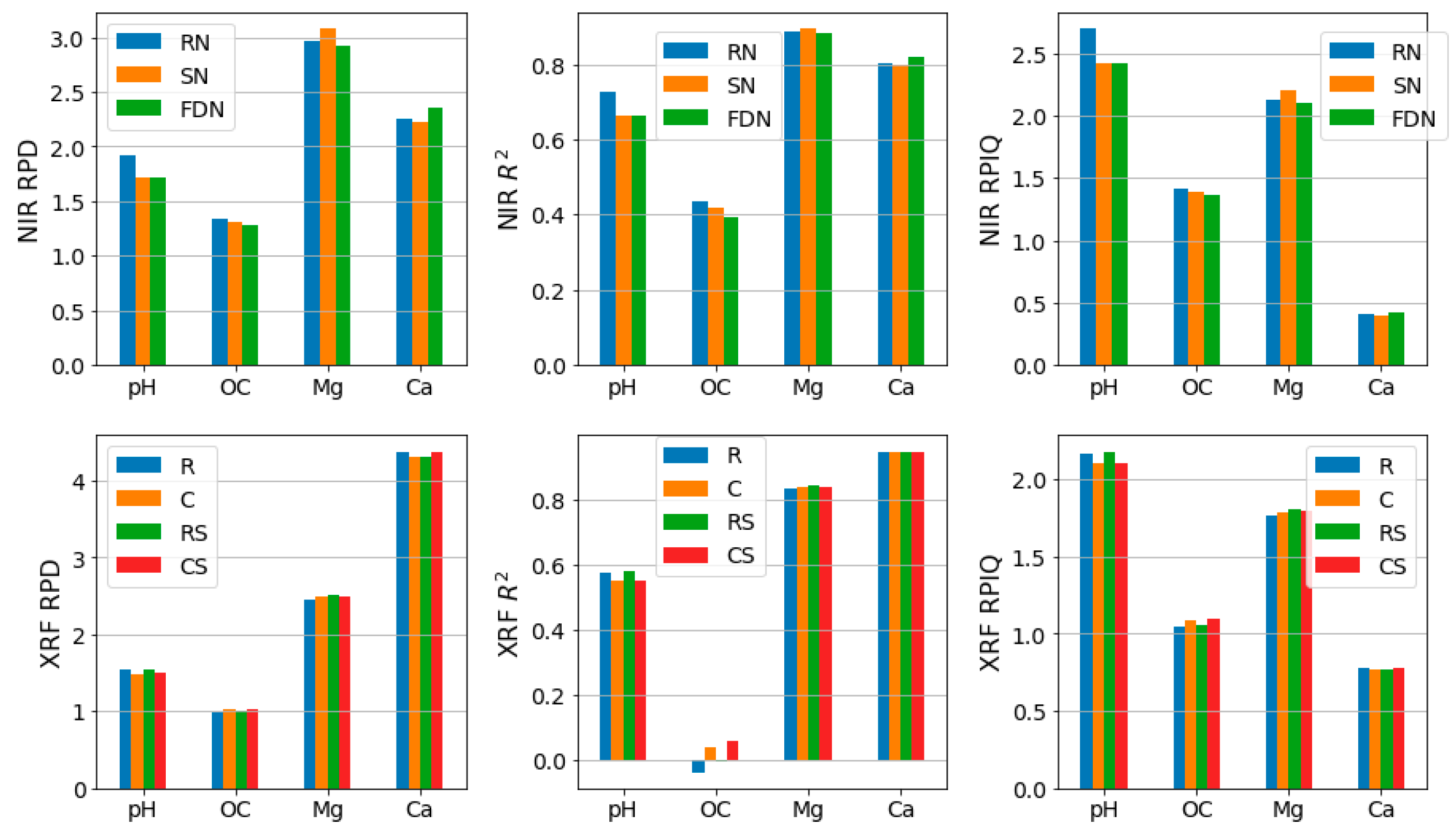
Figure 11.
The selected spectral and energy ranges for prediction of pH, organic carbon (OC), magnesium (Mg), and calcium (Ca) using (a) visible-near-infrared (vis-NIR) and (b) X-ray fluorescence (XRF).
Figure 11.
The selected spectral and energy ranges for prediction of pH, organic carbon (OC), magnesium (Mg), and calcium (Ca) using (a) visible-near-infrared (vis-NIR) and (b) X-ray fluorescence (XRF).
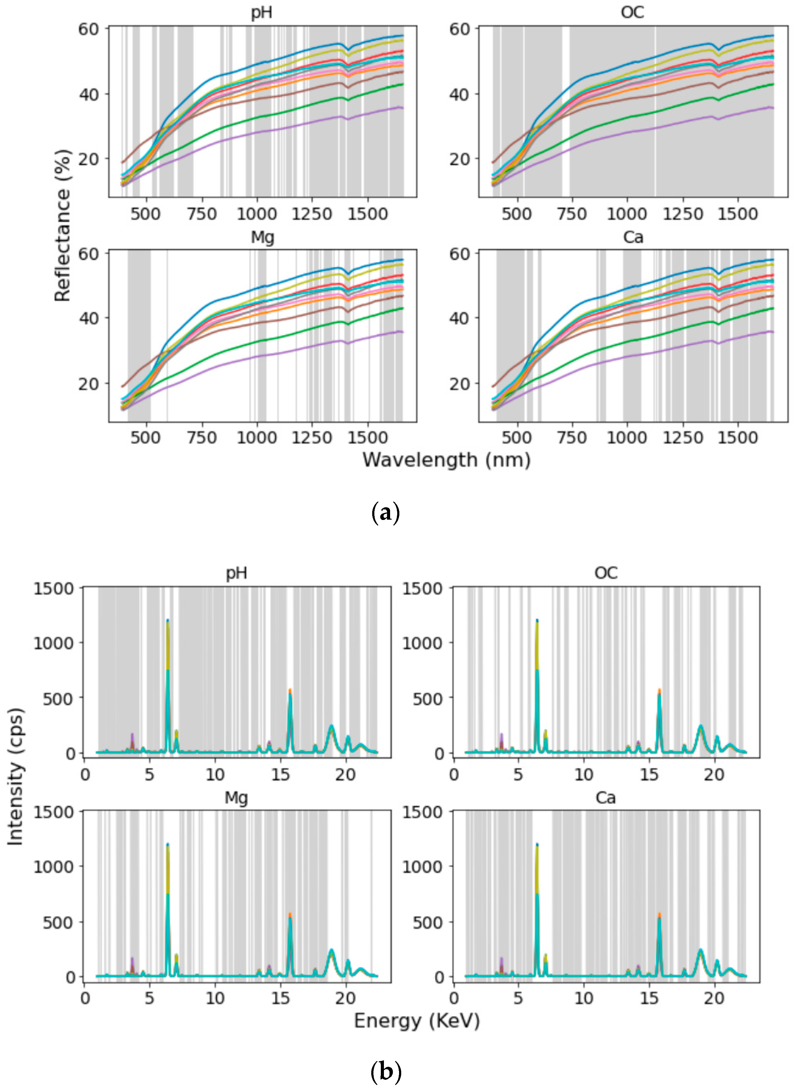
Figure 12.
Comparison of single-sensor partial least squares (PLS) modeling of visible-near-infrared (NIR) and X-ray fluorescent (XRF) with different data fusion schemes including outer product analysis (OPA), Granger–Ramanathan (GR), and least squares (LS) in terms of (a) root mean square error (RMSE), (b) ratio of performance to inter-quartile (PRIQ), (c) coefficient of determination (R2), and (d) ratio of performance to deviation (RPD). The soil attributes are: pH, organic carbon (OC), magnesium (Mg), and calcium (Ca).


Figure 13.
Outer product (OP) of the visible-near-infrared (vis-NIR) spectrum of a soil sample and its X-ray fluorescent (XRF) spectrum.
Figure 13.
Outer product (OP) of the visible-near-infrared (vis-NIR) spectrum of a soil sample and its X-ray fluorescent (XRF) spectrum.
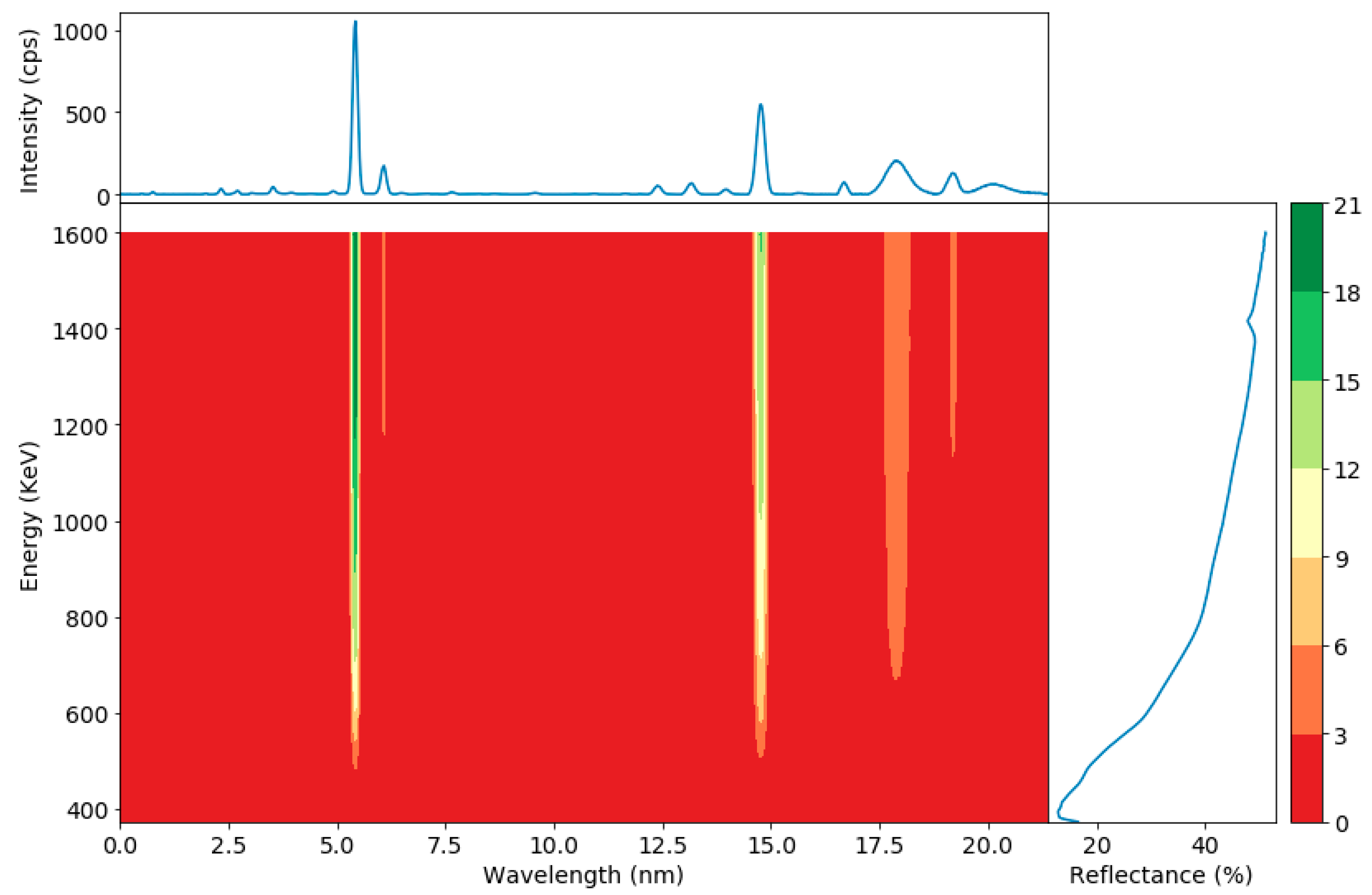
Figure 14.
The correlation between the residuals of the predictions given by visible-near-infrared (vis-NIR) and X-ray fluorescence (XRF) models.
Figure 14.
The correlation between the residuals of the predictions given by visible-near-infrared (vis-NIR) and X-ray fluorescence (XRF) models.

Table 1.
The information of the study fields in different areas of Flanders in Belgium.
| Field Name | Location | Date of Sampling (2018) | No. of Samples | Crop Type | Soil Texture | Average MC * (%) | Average OC ** (%) |
|---|---|---|---|---|---|---|---|
| Bottelare | Melle | Nov. | 23 | Maize | Light loam to light clay | 14.64 | 1.60 |
| Thierry | Moeskroen | Aug. | 13 | Wheat | Light sandy to sandy loam | 15.56 | 1.66 |
| Watermachine | Veurne | Aug. | 19 | Wheat | Heavy clay | 19.86 | 1.35 |
| Beers | Veurne | Aug. | 38 | Oil seed rape | Heavy clay | 19.30 | 1.29 |
| Kouter | Huldenberg | Jul./Aug. | 40 | Burley | Silt to silt loam | 3.63 | 1.10 |
| Gingelomse | Landen | Dec. | 37 | Barley | Light to heavy loam | 22.79 | 1.34 |
| Dal | Landen | Dec. | 21 | Sugar beet | Light to heavy loam | 23.02 | 1.38 |
| Kattestraat | Landen | Aug. | 19 | Barley | Light to heavy loam | 8.75 | 1.47 |
| Grootland | Landen | Oct. | 57 | Wheat | Light to heavy loam | 19.67 | 1.16 |
* MC: Moisture content. ** OC: Organic carbon.
Table 2.
The fields that were used for validation of the prediction models of each soil attribute.
| Attribute | Validation Fields |
|---|---|
| pH | Grootland, Gingelomse, Thierry |
| OC | Grootland, Kattestraat, Thierry |
| Mg | Grootland, Watermachine, Thierry |
| Ca | Kouter, Dal, Watermachine |
OC: organic carbon; Mg: magnesium; Ca: calcium; Na: sodium.
Table 3.
The number of the latent variables used in the partial least squares (PLS) models of individual visible-near-infrared (vis-NIR) and X-ray fluorescence (XRF) spectra and fusion models by outer product analysis (OPA) with full spectra as input (OPA-FS) and selected spectra ranges as input (OPA-SS).
| Vis-NIR | XRF | OPA-FS | OPA-SS | ||||||
|---|---|---|---|---|---|---|---|---|---|
| Pre-Processing | R | S | FD | R | C | RS | CS | ||
| pH | 2 | 2 | 4 | 6 | 2 | 6 | 2 | 2 | 2 |
| OC | 4 | 4 | 3 | 5 | 5 | 5 | 5 | 2 | 3 |
| Mg | 6 | 7 | 4 | 3 | 4 | 3 | 4 | 3 | 2 |
| Ca | 7 | 9 | 4 | 5 | 6 | 5 | 6 | 2 | 3 |
The pre-processing methods are raw (R), smoothed (S), first derivative (FD), Compton normalization (C), raw-smoothing (RS), and Compton-normalization-smoothing (CS). OC: organic carbon; Mg: magnesium; Ca: calcium.
Table 4.
The Pearson correlation coefficient (ρ) between the residuals of the predictions given by visible-near-infrared (vis-NIR) and X-ray fluorescence (XRF) models.
Table 4.
The Pearson correlation coefficient (ρ) between the residuals of the predictions given by visible-near-infrared (vis-NIR) and X-ray fluorescence (XRF) models.
| pH | OC | Mg | Ca | |
|---|---|---|---|---|
| ρ | 0.34 | 0.38 | 0.17 | −0.2 |
OC: organic carbon; Mg: magnesium; Ca: calcium; Na: sodium.
Publisher’s Note: MDPI stays neutral with regard to jurisdictional claims in published maps and institutional affiliations. |
© 2021 by the authors. Licensee MDPI, Basel, Switzerland. This article is an open access article distributed under the terms and conditions of the Creative Commons Attribution (CC BY) license (https://creativecommons.org/licenses/by/4.0/).
Share and Cite
MDPI and ACS Style
Javadi, S.H.; Mouazen, A.M. Data Fusion of XRF and Vis-NIR Using Outer Product Analysis, Granger–Ramanathan, and Least Squares for Prediction of Key Soil Attributes. Remote Sens. 2021, 13, 2023. https://doi.org/10.3390/rs13112023
AMA Style
Javadi SH, Mouazen AM. Data Fusion of XRF and Vis-NIR Using Outer Product Analysis, Granger–Ramanathan, and Least Squares for Prediction of Key Soil Attributes. Remote Sensing. 2021; 13(11):2023. https://doi.org/10.3390/rs13112023
Chicago/Turabian StyleJavadi, S. Hamed, and Abdul M. Mouazen. 2021. "Data Fusion of XRF and Vis-NIR Using Outer Product Analysis, Granger–Ramanathan, and Least Squares for Prediction of Key Soil Attributes" Remote Sensing 13, no. 11: 2023. https://doi.org/10.3390/rs13112023
Note that from the first issue of 2016, this journal uses article numbers instead of page numbers. See further details here.