Article

Remotely Sensed Ecological Protection Redline and Security Pattern Construction: A Comparative Analysis of Pingtan (China) and Durban (South Africa)

1
School of Geographical Science, Fujian Normal University, Fuzhou 350007, China
2
Department of Transdisciplinary Science and Engineering, School of Environment and Society, Tokyo Institute of Technology, Ookayama 2-12-1 W8-5, Meguro, Tokyo 152-8552, Japan
3
Irrigation and Hydraulics Engineering Department, College of Engineering, Mansoura University, 60 Elgomhoria Street, Mansoura 35516, Egypt
4
Fujian Provincial Key Laboratory of Subtropical Resources and Environment, Fujian Normal University, Fuzhou 350007, China
5
College of Environmental Science & Engineering, Fujian Normal University, Fuzhou 350007, China
6
Faculty of Geography, Yunnan Normal University, Chenggong District, Kunming 650500, China
7
Center of Sustainable Forest Management and Remote Sensing, Volga State University of Technology, 424000 Yoshkar-Ola, Russia
8
Council for Geoscience, 280 Pretoria Street, Silverton, Private Bag X112, Pretoria 0001, South Africa
*
Author to whom correspondence should be addressed.
Remote Sens. 2021, 13(15), 2865; https://doi.org/10.3390/rs13152865
Submission received: 22 May 2021 / Revised: 5 July 2021 / Accepted: 7 July 2021 / Published: 22 July 2021
(This article belongs to the Special Issue Geographic Data Analysis and Modeling in Remote Sensing)

Abstract

:
The unprecedented regional urbanization has brought great pressure on the ecological environment. Building an ecological security pattern and guide regional land and space development is an important technique to ensure regional ecological security and stability to achieve sustainable development. In this study, the Pingtan Island of China and the Durban city of South Africa were chosen as case study area for a comparative study of different scales. The importance of ecosystem services and ecological sensitivity were evaluated, respectively. The core area of landscape which is vital for ecological function maintenance was extracted by morphological spatial pattern analysis (MSPA) and landscape connectivity analysis. Furthermore, the ecological sources were determined by combining the results of ecological protection redline delimitation and core area landscape extraction. The potential ecological corridors were identified based on the minimum cumulative resistance model, and the ecological security pattern of study areas was constructed. The results showed that the ecological protection redline areas of Pingtan and Durban were 42.78 km2 and 389.07 km2, respectively, which were mainly distributed in mountainous areas with good habitat quality. Pingtan ecological security pattern is composed of 15 ecological sources, 16 ecological corridors, 10 stepping stone patches and 15 ecological obstacle points. The total length of corridors is 112.23 km, which is radially distributed in the form of “one ring, three belts”. The ecological security pattern of Durban is composed of 15 ecological sources, 17 ecological corridors, 11 stepping stone patches and 18 ecological obstacle points. The total length of corridors is 274.25 km, which is radially distributed in the form of “two rings and three belts”. The research results can provide an important reference for the land space construction planning and ecological restoration projects in Pingtan and Durban.

Graphical Abstract

1. Introduction

The combined impact of urbanization, the rapid growth of population and land use dramatic changes led to ecological problems including forest and grass degradation, loss of biodiversity and aggravation of soil erosion. This has brought about dramatic changes in the ecological environment and brought great pressure on human life. The ecological environment is facing great challenges, threatening people’s life and the development of the country. Protecting regional ecological security has become an important work to ensure regional stability and sustainable development.
Ecological security patterns (ESP) refer to the spatial layout scheme of the point, line and plane composed of the key parts of the natural landscape [1]. It is of great significance to protect the regional biodiversity, maintain the functional integrity of the regional ecosystem and realize the smart growth of the city [2]. The related theories and methods of ESP were further improved by Kongjian Yu [3], and scholars have carried out a lot of research [4,5,6]. At present, using the minimum cumulative resistance (MCR) model to extract ecological sources and identify potential ecological corridors has gradually become the main method of ESP construction [7,8]. As the starting point of species diffusion and migration, the ecological source area is a key component of ESP [9]. At present, the identification methods of ecological sources can be divided into direct identification method and comprehensive evaluation identification method. The direct identification method is to directly identify the important ecological land such as nature reserves, scenic spots and forest parks in the regional planning as the ecological sources [10]. This method ignores the overall ecological environment of the study area, and the division of nature reserves and scenic spots is relatively new and slow. With time, the divided nature reserves lack timeliness. Due to the influence of human factors, the ecological environment may have changed, which leads to the inaccurate identification of ecological sources. The comprehensive evaluation and identification is to comprehensively evaluate the ecological environment quality of the study area from multiple factors and angles. The patch with better ecological quality is identified as the ecological sources by using the superposition of spatial analysis technology [11,12]. The evaluation system based on comprehensive factors can be used to evaluate the quality of regional ecological environment. It comprehensively reflects the regional ecological security situation from different angles and effectively identifies the source area. In recent years, some scholars have introduced the ecological protection redline and morphological analysis method into the study of ecological security patterns. It provided new reference and research ideas for the extraction of ecological sources.
In 2011, China put forward the concept of ecological protection redline, which provides a new idea for ecological environment protection with bottom-line thinking [13]. As an important innovation of the ecological protection system, the ecological protection redline delimits the ecological control area with the bottom line thinking [14]. It can ensure the stability of regional ecosystem function, maintain the pattern of ecological security. The implementation of ecological protection redline policy is conducive to promoting the balance of resources and environment and the unification of economic and ecological benefits [15,16]. Therefore, combining with the ecological protection redline to construct the regional ecological security pattern can better control the regional ecological elements and maintain the regional ecological security.
In this paper, Pingtan Island in Fujian Province of China and Durban in South Africa are selected as research areas. The random forest method is used for land use classification based on Landsat 8 oli image. Based on the evaluation of ecosystem service function importance and ecological sensitivity, GIS spatial analysis technology is used to delimit the ecological protection redline. Morphological spatial pattern analysis (MSPA) combined with landscape connectivity evaluation was used to identify the core area landscape. The ecological source area was extracted by combining the results of MSPA and the ecological protection redline. The extraction of ecological sources is based on ecosystem service function, ecological sensitivity and landscape connectivity of core area. Considering not only the ecosystem service value to humans and the response of ecological process to environmental change, but also the structure and function of patches, the core ecological patches with high regional connectivity are extracted. In addition, there is a lack of evaluation on the importance of ecological sources in previous studies. In this paper, based on the data of Zhuhai-1 hyperspectral satellite, the vegetation index of Pingtan red-edge was calculated to evaluate the ecological sources. The potential ecological corridors were identified based on the MCR model, and the relative importance of corridors was determined based on the gravity model. Taking the intersection of corridors as the ecological nodes and the intersection of corridors and main roads as the ecological obstacle points, the ecological security patterns of Pingtan Island and Durban are constructed, respectively. The results can provide the basis for the planning of land space and ecological security pattern of Pingtan and Durban, and also provide the reference for the construction of regional ecological security pattern.

2. Materials and Methods

2.1. Survey and Data Sources of Study Areas

2.1.1. Study Area

Pingtan Island (25°15′–25°45′ N, 119°32′–120°10′ E) is the main area in Pingtan County (Figure 1a). Pingtan Island is located in the eastern part of Fujian Province, with an area of 267.13 km2. The terrain is low and flat, with an annual average temperature of 19.0–19.9 °C. It belongs to the subtropical marine monsoon climate, with an annual rainfall of 900–1200 mm and distinct dry and rainy seasons. The soil types of the island are mainly latosol and coastal aeolian sandy soil, and the vegetation is mainly plantation planted in the 1960s. The vegetation community is single and has been degraded. As the closest Chinese mainland to Taiwan, it is an important window to Taiwan trade. In 2009, it was granted the Pingtan comprehensive experimentation area. With the development of Pingtan, the dramatic change of land use has brought great challenges to the biodiversity and ecosystem services in Pingtan.
Durban (Figure 1b) is a port city in KwaZulu Natal province, South Africa, with an area of 2292 km2. The climate of Durban is subtropical, with an annual rainfall of about 1000 mm, an average annual temperature of 16.0–25 °C and abundant sunshine [17,18]. It is the first beach city on the east coast of Africa. The rapid development of suburban industry has led to the recovery of the mainland economy. The establishment of the Durban Investment Promotion Association (DIPA) has promoted the development of Durban into a modern pioneering city. At the same time of economic development, the ecological environment of Durban is facing many pressures. Among them, the most prominent problems are species habitat destruction, alien invasive species and pollution [19,20].
Pingtan is an island city, while Durban is a coastal city, which has coastal commonness, and both cities are in the subtropical region. Pingtan and Durban are both in special geographical location. Pingtan is an important window for China’s mainland trade with Taiwan (China), while Durban is the gateway port city of South Africa. In recent years, Pingtan and Durban have developed rapidly. At the same time, the ecological security of the two places has also been greatly challenged. Therefore, how to coordinate the development of urban social economy and ecological security is very important.

2.1.2. Data Sources

The main data used in this paper are shown in Table 1, including Landsat 8 oli image data of Pingtan (imaging time: 2 April 2017) and DEM data, with a spatial resolution of 30 m (from geospatial data cloud: http://www.gscloud.cn/ (accessed on 25 January 2021)). Pingtan soil data, with a spatial resolution of 30 m (from Nanjing Soil Research Institute: http://www.issas.ac.cn/ (accessed on 7 March 2021)). Pingtan basic geographic information data (from the China Geographic Information Resources Directory Service System: https://www.webmap.cn/ (accessed on 27 January 2021)) and Pingtan administrative division data. Zhuhai-1 satellite image data (imaging time: 16 March 2020; Spatial resolution: 10 m). Landsat 8 oli image data of Durban (imaging time: 3 June 2017) and DEM data, with a spatial resolution of 30 m (from the United States Geological Survey (USGS): (https://earthexplorer.usgs.gov/ (accessed on 18 April 2021)). Soil data of Durban, with a spatial resolution of 1 km (from Harmonized World Soil Database: http://www.fao.org/ (accessed on 18 April 2021)). The acquired soil data were drawn manually, and the resolution was converted to 30 m. Basic geographic information data (from the open street map: (http://openstreetmap.org/ (accessed on 20 April 2021))) and the data of administrative divisions in Durban. Landsat 8 oli image data was used for land use classification and vegetation coverage calculation after remote sensing image preprocessing. According to the actual situation of Pingtan Island and Durban, the land use types were divided into six categories: Agriculture, Forest land, Build-up land, Grassland, Water body and Undeveloped land. The random forest classifier was used for classification. After testing, the overall classification accuracy is more than 88%, which meets the research needs. DEM was used to extract elevation and slope. Basic geographic information data was used to extract road and railway networks. Zhuhai-1 satellite image data was used to calculate the red-edge vegetation index.
After map projection and clipping, the extracted data was converted into 30 m × 30 m grid data.

2.2. Delimitation Method of Ecological Protection Redline

According to “Ecological Redline Delimitation Guide” issued by the general office of the Ministry of environmental protection of China, the importance of ecosystem service function and ecological sensitivity of study areas were evaluated. According to the references [21,22] and the characteristics of ecological environment in study areas, three indicators were selected for evaluating the importance of ecosystem services and six factors for the ecological sensitivity (Table 2). The flow chart of ecological protection redline delimitation is shown in Figure 2.

2.2.1. Ecosystem Services Evaluation

Based on the characteristics of study areas and the availability of data, the importance of ecosystem services was evaluated by three factors: soil and water conservation function, carbon sequestration and oxygen release function and biodiversity maintenance function. Soil erosion, carbon storage and habitat quality were used to characterize the three factors.

Soil Erosion

The universal soil loss equation (USLE) was used to evaluate the soil erosion in study areas:
A = R · K · L · S · C · P
In the formula, A is annual soil erosion, unit: t/hm2; R is rainfall erosivity factor, unit: MJ mm/(hm2·h a); K is soil erodibility factor, unit: t h/(MJ mm); L S is slope length factor; C is vegetation and management factor [23]; P is soil conservation factor [24].

Carbon Storage

The carbon storage module based on invest model is used to calculate the carbon storage in study areas:
C k t = C k a b o v e + C k b e l o w + C k s o i l
C = 0 5 S k + C k t
where, C k t is the total carbon density of land use type k (t/hm2); C k a b o v e is the aboveground biomass carbon density of k (t/hm2); C k b e l o w is the density of underground biological carbon of k (t/hm2); C k s o i l is the soil carbon density of k (t/hm2); C is the carbon storage of study areas (t); S k is the area of land use type k (hm2). Based on the research results of Li, Wu, Ringius and Johnson, the soil carbon density data of study areas is determined [25,26,27,28].

Biodiversity Maintenance Function

The habitat quality module based on invest model was used to evaluate the habitat quality of study areas:
Q i j = H j [ 1 D i j 2 D i j 2 + k 2 ]
where: Q i j is the habitat quality of the i th grid of land use type j ; H j is the habitat suitability of land type j ; D i j is the habitat stress level of grid i inland type j . In this paper, build-up land, agriculture and undeveloped land are selected as the threat factors; k is the semi saturation constant, which is set as 0.5 here.
According to the natural breakpoint method, the evaluation results of three different ecosystem services were classified into five grades, and the importance of each grade decreased gradually. The most important levels of ecosystem service function factors were extracted and intersected to get the ecological redline.

2.2.2. Ecological Sensitivity Assessment

Combined with the actual situation of study areas and the reference literature [29], six ecological sensitivity indices were selected for ecological sensitivity evaluation (Table 3). Among them, the elevation and slope were calculated by DEM. The distance from railway and important water area was calculated by buffer analysis. Different land types were assigned values to divide the ecological sensitivity of different land-use types. Fractional vegetation coverage was calculated by remote sensing image data. The comprehensive index evaluation method was used to evaluate the six selected indices [30]. The calculation formula is as follows:
S m = n = 1 m   w n × x m n
where, w n is the weight of the n th evaluation factor; x m n is the value of the n th evaluation factor on the m th pixel, S m is the comprehensive evaluation result of the ecological sensitivity of the m th pixel. Weight w n the setting was determined by the analytic hierarchy process combined with relevant reference [31]. The six selected factors were weighted and superimposed to obtain the comprehensive evaluation results of ecological sensitivity. The results were graded and assigned according to the natural breakpoint method, and the extremely sensitive areas were extracted as the ecological protection redline areas.

2.3. Ecological Sources Identification

The morphological spatial pattern analysis (MSPA) method [32,33] was used to extract the core patches with the best ecological function. In addition, the landscape connectivity of patches in the core area was analyzed [32,33], so as to determine the ecological sources [34].

2.3.1. Core Area Patch Extraction Based on MSPA Method

First, the raster data of land use types were reclassified, and the forest land among the six land types was taken as the foreground value, and the other land types were taken as the background value. It was imported into Guidos toolbox (Joint Research Centre, Ispra, Italy.)for MSPA analysis, and seven kinds of landscapes with different functions were obtained.

2.3.2. Evaluation of Landscape Connectivity

The grid data from MSPA analysis was converted into vector data, and the patches in the core area were extracted, and the landscape connectivity was evaluated by Conefor 2.6 (Universidad Politécnica de Madrid, Madrid, Spain.). The calculation formula is as follows:
P C = i = 1 n j = 1 n a i × a j × P i j A L 2
d P C = P C P C r e m o v e P C × 100 %
Among them, a i and a j represent the area of patch i and patch j , respectively; n represents the total number of regional patches; P i j is the maximum probability of species directly spreading between patch i and patch j ; A L is the total land area of study areas P C r e m o v e represents the possible connectivity index for removing this patch. P C is the possible connectivity index, and d P C is the plaque importance index. The larger the value, the higher the importance of the patch.

2.4. Minimal Cumulative Resistance Model

2.4.1. Resistance Surface Construction

The Minimal Cumulative Resistance (MCR) model reflects the possibility of species passage in the landscape by calculating the cost of species moving from the ecological sources to the destination [35]. The calculation formula of the MCR model is as follows:
M C R = f m i n v = n u = m D u v × R u
Among them, D u v is the spatial distance from the source point u to the spatial unit v ; R u is the resistance coefficient of the spatial unit u to the movement of the species.
The key to the construction of the Minimal Cumulative Resistance model is the selection of ecological sources and the construction of the resistance surface. The disturbance of human activities and the quality of the ecological environment are the main sources of resistance in the movement of species. Based on reference to related literature, this paper established a basic resistance surface according to the degree of impact of different landscape types by human activities (Table 4) [36,37]. The fractional vegetation coverage and habitat quality were used to correct the basic resistance surface to construct the final resistance surface. The specific formula is as follows:
R i = F V C i F V C j × H Q i H Q j × R 0
where: R i represents the revised ecological resistance coefficient, F V C i is the fractional vegetation coverage of grid unit i , F V C n is the average fractional vegetation coverage of land use type j corresponding to grid unit i ; H Q i is the habitat quality index of grid unit i , H Q j is the average value of the habitat quality index of land use type j corresponding to grid unit i ; R 0 is the relative resistance coefficient of the grid before correction.

2.4.2. Resistance Surface Construction Extraction of the Ecological Corridors

Based on the cost distance module of Arcgis 10.2 (Environmental Systems Research Institute, Redlands, CA, USA), the resistance surface of cumulative consumption between source areas was calculated and the potential ecological corridors was identified. Based on the gravity model, the interaction strength between patches in the ecological source area was calculated. In addition, the important ecological corridors were extracted to construct the ecological security pattern [37,38,39]. The formula is as follows:
G u v = N u × N v D u v 2 = [ 1 P u × ln ( S u ) ] [ 1 P v × ln ( S v ) ] ( L u v L m a x ) 2 = L m a x 2 ln ( S u ) × ln ( S v ) L u v 2 P u P v
where: N u and N v are the weights of patches u and v ; D u v is the standardized value of the corridors resistance between patches u and v ; P u and P v represent the overall resistance values of patches u and v , respectively; S u and S v are the area of the patches u and v ; L U V is the cumulative resistance value of the corridors between the patches u and v ; L m a x is the maximum value of the cumulative resistance in all the corridors; G u v represents the interaction strength between the patches u and v .

2.5. Ecological Sources Identification Calculation of Red-Edge Vegetation Index Based on Hyperspectral Image

In the 1980s, the emergence of hyperspectral remote sensing injected new vitality into the field of remote sensing [40]. Hyperspectral remote sensing has the advantages of rich information and high spectral resolution, which greatly improves the accuracy and reliability of quantitative remote sensing [41]. The development of hyperspectral technology has further enriched the study of vegetation index [42,43]. Some scholars found that the red edge region between Red and NIR band has a good correlation with chlorophyll, leaf area index, and other parameters. These indices characterize the growth status of green plants, which can be used to monitor the growth status of green plants. The growth and health status of vegetation reflect the ecological security status of the region to a large extent. Therefore, the hyperspectral data of Zhuhai-1 was used to monitor the growth and health of vegetation in Pingtan through the red-edge vegetation index. In addition, the ecological level of different ecological sources was evaluated accordingly.
Four kinds of red-edge vegetation indices were selected for calculation, including Red-edge Normalized Difference Vegetation Index (NDVIred-edge), Modified Red-edge Simple Ratio Index (MSRred-edge), Chlorophyll Red-edge Index (CIred-edge) and novel Inverted Red-edge Chlorophyll Index (IRECI). Since some bands needed for red-edge vegetation index could not be obtained from Zhuhai-1 satellite, the nearest band was used instead. The specific calculation formula is shown in Table 5. According to the formula in Table 5, the red-edge vegetation indices were calculated, and the results were normalized to eliminate the errors caused by different vegetation index dimensions.

3. Results

3.1. Analysis of Ecosystem Service Function and Ecological Sensitivity

3.1.1. Analysis of the Importance of Ecosystem Services

According to the method mentioned in Section 2.2.1, the soil erosion, habitat quality and carbon storage of Pingtan and Durban were calculated, respectively. The results are shown in the Figure 3. It can be seen from the Figure 3a,d that Pingtan is more seriously eroded in the western coastal area, while Durban is more seriously eroded in the southeast coastal area, which is greatly disturbed by human activities. Figure 3b,e shows that in Pingtan and Durban forest land and grassland had better habitat quality, they are the important parts to maintain the stability of ecosystem. Figure 3c,f shows that the carbon storage of Pingtan and Durban is higher in the area where forest land is concentrated. The value of carbon fixation and oxygen release of forest is the basis of life support of the earth.
The three indices were graded by natural breakpoint method, and the regions with the strongest ecosystem service function were extracted for superposition. According to the superposition results, the final redline of ecosystem service function importance was drawn.

3.1.2. Analysis of the Ecological Sensitivity

According to the indices selected in Section 2.2.2, index extraction and sensitivity grading were carried out, and the sensitivity grading results of each index are shown in Figure 4 and Figure 5. According to the weight assigned by AHP, the final ecological sensitivity grading result is obtained by weighted superposition, as shown in Figure 6. It can be seen from the figure that the ecologically sensitive areas in Pingtan are mainly concentrated and dense woodland, and the main drinking water source area of Pingtan is Sanshiliujiao Lake. The ecological sensitive areas in Durban are mainly forest land areas with higher inland altitude and close to main rivers.

3.2. Analysis of Ecological Protection Redline

3.2.1. Pingtan Ecological Protection Redline Analysis

According to the above research methods, the ecological function importance and ecological sensitivity of Pingtan and Durban were evaluated, respectively. Combined with the actual situation of study areas, the small patches with an area of fewer than 0.5 km2 (Pingtan) and 2 km2 for (Durban) were deleted.
The results of the ecological protection redline based on ecosystem service function evaluation are shown in Figure 7a. The results of the ecological protection redline based on the comprehensive evaluation of ecological sensitivity are shown in Figure 7b. The area statistics of ecological sensitivity evaluation results are shown in Table 6. Among them, non-sensitive areas and low sensitive areas account for more than 55% of the area of Pingtan Island, which indicates that the ecological sensitivity of Pingtan Island is generally good. In addition, highly and extremely sensitive areas account for 25.57% of the total area. These areas are ecologically fragile areas in Pingtan, and the ecological environment is easily affected by human and natural factors. The results of the ecological protection redline based on ecosystem service importance assessment and ecological sensitivity assessment were superimposed. As shown in Figure 7c, the ecological protection redline area is 42.78 km2, accounting for 15.01% of the total land area of Pingtan Island. It is mainly distributed in the mountain areas of Pingtan plain town, Zhonglou Township and Liushui town in the north and Beicuo town in the southwest. These areas are the main forest distribution areas in Pingtan, with good ecological environment quality, and are also important areas to maintain biodiversity and ecosystem stability. It should be protected within the redline of ecological protection. There is no organic connection between the north and the south of the ecological protection redline area, which is not conducive to the material and energy exchange within the region.

3.2.2. Durban Ecological Protection Redline Analysis

The results of the ecological protection redline in Durban according to ecosystem service function assessment are shown in Figure 8a. The results of the ecological protection redline based on the comprehensive evaluation of ecological sensitivity are shown in Figure 8b. The statistical results of ecologically sensitive areas are shown in Table 6. Among them, the non-sensitive area and low sensitive area accounted for 39.27% of the total area of Durban, which is lower than Pingtan. The extremely sensitive area accounted for 18.17% of the total area, which is higher than Pingtan, indicating that the overall ecological sensitivity of Durban is more sensitive than Pingtan. The ecological environment of Durban is more vulnerable to human and natural factors.
As shown in Figure 8c, the redline of ecological protection in Durban covers an area of 389.07 km2, accounting for 17.17% of the total land area of the city. It is mainly distributed in the mountainous areas in the central and northwest parts of the city. These areas are of good ecological environment quality and important for maintaining biodiversity and ecosystem stability. Compared with Pingtan, the ecological protection redline area is more evenly distributed, but the Northeast coastal area is lacking contact with the inland. This area is the main cultivated land distribution area in Durban, and is greatly affected by human disturbance.

3.3. Analysis of Ecological Sources

In this paper, seven different landscape types were obtained through MSPA analysis (Figure 9). According to the classification statistics of different landscape types (Table 7), the core areas of Pingtan and Durban are 43.11 km2 and 286.42 km2, respectively, accounting for 51.54% and 53.66% of each prospect element type. According to the attribute selection, the patches in the core area were exported and input into Conefor 2.6 (Universidad Politécnica de Madrid, Madrid, Spain). The importance index DPC of the patches in the core area was calculated. The ecological protection redline patches with an area of more than 1 km2 (Pingtan) and more than 8 km2 (Durban) and the patches with DPC greater than 5.0 (Pingtan and Durban) were taken as the ecological source areas, respectively. As shown in Figure 10, the extracted Pingtan ecological source area is 31.95 km2, accounting for 11.2% of the total area of Pingtan Island. The extracted Durban ecological source area is 108.18 km2, accounting for 4.78% of the total area of Durban. It can be seen from Figure 10 that the landscape connectivity of the Pingtan region is good. The connectivity of forest landscape in the north and southwest region is strong, while the connectivity of landscape in the middle and southeast region is weak. The patches lacking connection between different regions have fault phenomenon, which is not conducive to species migration. Among them, patch 10, patch 9 and patch 11 act as bridges between North and south, east and west, respectively. They play an important role in maintaining the material and energy exchange between different ecological sources. It can be seen from Figure 9b that the landscape connectivity of woodland in the Northwest and central part of Durban is better than that in the South and eastern coastal area, and the forest distribution is more concentrated than that in Pingtan. Compared with Pingtan, the patch area of forest in Durban is smaller and the distribution is more scattered.

3.4. Analysis of Ecological Corridors

3.4.1. Analysis of Pingtan Ecological Corridors

As shown in Figure 11a, a total of 105 potential ecological corridors were generated by using the MCR model. There are a large number of paths overlapping in the potential ecological corridors with high redundancy. The gravity model was used to evaluate the importance of potential corridors. The results are shown in Table 8. It can be seen from Table 8 that the importance of patches varies greatly, and the importance of adjacent patches is much greater than that of patches with a long distance. Corridor construction costs a lot of resources and costs. According to the results of the gravity model, the replaceable part of the potential ecological corridors was eliminated, and the redundancy between corridors was reduced. Finally, 16 ecological corridors were obtained. As shown in Figure 12a, the total length of the corridors is 112.23 km, which is radially distributed in the form of “one ring and three belts”. Ecological process is affected by human activities and natural factors, among which human factors have a greater impact on the ecological process. To ensure that the corridors width is suitable for species migration to the greatest extent, buffer analysis was used to calculate the area proportion of each land use type under different corridor widths. As shown in Table 9, when the corridor width increases, the proportion of build-up land and agriculture increases, and the corridor is also affected by human activities. According to the research of Ford et al. on the corridor width [47], combined with the species situation in Pingtan, the corridor width is determined as 100~300 m. The corridor width can provide better migration space for species, and is less affected by human activities.
The ecological node is the most vulnerable place of regional ecological function [48,49]. In this paper, the intersection of corridors was selected as the ecological node, and a total of 10 ecological nodes were selected. Ecological obstacle points are the corridor breakpoints that affect species migration and material and energy exchange between source areas. In this paper, the intersection points of main roads and ecological corridors were extracted as ecological obstacle points, and a total of 15 obstacle points were extracted.

3.4.2. Analysis of Durban Ecological Corridors

As shown in Figure 11b, a total of 120 potential ecological corridors were generated by using the MCR model. The results of the importance evaluation of potential corridors by using the gravity model are shown in Table 10. According to the results of the gravity model, the replaceable parts of potential ecological corridors were eliminated, and the redundancy between corridors was reduced. Finally, 17 ecological corridors were obtained. As shown in Figure 12b, the total length of the corridors is 274.25 km, which is radially distributed with “two rings and three belts”. The statistical results of the area proportion of various land-use types under different widths of the corridors are shown in Table 11. When the corridor width increases, the area proportion of build-up land and agriculture increases, and the corridor is also affected by human activities. The corridor width was determined as 400–800 m according to the actual situation. According to the intersection of corridors and corridors and main roads, 11 ecological nodes and 18 ecological obstacle points were extracted.

3.5. Analysis of Red-Edge Vegetation Index

In order to further evaluate the ecological security status of Pingtan, the hyperspectral satellite image of Zhuhai-1 was used to calculate four red-edge vegetation indices. The red-edge vegetation indices were normalized, and the results are shown in Figure 13. The Zhuhai-1 satellite images used in the study did not cover the whole study area. The mean values of vegetation indices of different land-use types were taken in the study, which approximately represented the mean values of all classes in the whole study area. Based on the classification results and the calculation results of vegetation index, the mean values of red-edge vegetation index of different land types were calculated, as shown in Table 12. It can be seen from Table 12 that the average value of four vegetation indices of forest land in Pingtan is the highest, while the average value of build-up land is the lowest. The order of Red-edge Normalized Difference Vegetation Index (NDVIred-edge) and Red-edge Simple Ratio Index (MSRred-edge) was forest > water > grassland > agriculture > undeveloped land > build-up land. The order of Chlorophyll Red-edge Index (CIred-edge) and novel Inverted Red-edge Chlorophyll Index (IRECI) was forest > grassland > water > agriculture > undeveloped land > build-up land.
Based on the results of ecological sources extraction and vegetation index, the average values of four red-edge vegetation indices in different ecological source areas were counted. The average values of the four vegetation indices were superimposed with equal weight to obtain the comprehensive vegetation index (VIS). Since the hyperspectral image does not cover the whole study area, the mean value of 14 source patches except source 2 is calculated, as shown in Table 13. The statistical results of the comprehensive vegetation index were visualized, as shown in Figure 14. It can be seen from Table 13 that source 12 is the ecological source patch with the highest mean value of comprehensive vegetation index, source 3 is the lowest. Source 12, 13 and 15 are the ecological source patches with higher vegetation index, while source 3, 4 and 5 are the ecological source patches with lower vegetation index. The vegetation index can reflect the growth and health status of plants. As an important component of the ecosystem, vegetation not only provides habitat and food sources for animals but also plays a role in regulating the balance of carbon and oxygen. Therefore, the ecological source areas with better growth and health status of vegetation play a more critical role in the ecological security pattern.

3.6. Analysis of the Ecological Security Pattern

3.6.1. Pingtan Ecological Security Pattern

Pingtan ecological security pattern is composed of ecological sources, ecological corridors, stepping stones and ecological protection redline. There are 16 corridors with a total length of 112.23 km, and the area of ecological protection redline is 42.78 km2. As can be seen from Figure 15a, except for some areas of patches 7, 9 and 10 which are not within the ecological protection redline, the other ecological source patches are within the ecological protection redline. From the results of red-edge vegetation indices, patches 12, 13 and 15 are ecological source patches with better vegetation growth and health. They are conducive to maintaining the integrity of the ecosystem, and the protection of these ecological source areas should be strengthened. From the results of the gravity model, the interaction between patch 3 and patch 4 is the strongest. The results show that the resistance of material and energy exchange between these patches is small and the possibility of species migration is high. Therefore, the construction of the corridors should be strengthened to avoid the damage caused by human factors. In addition, patch 9, patch 10 and patch 11, as the bridge connecting the north and south, east and west, play a mediating role in the communication between the endogenous areas of the island. Therefore, the protection of the corridors associated with them is also very important, which is of great significance to the construction of the overall ecological security pattern of Pingtan. Stepping stones were transformed from ecological nodes, and they are the rest patches in the process of species migration. It is necessary to carry out key construction to ensure the smooth progress of species migration. The ecological obstacle point is the break point in the corridors network, which affects the flow of ecological process and needs to be repaired by vegetation planting and other methods.

3.6.2. Ecological Security Pattern in Durban

In the construction of ecological security pattern in Durban, there are 17 corridors with a total length of 274.25 km; The ecological protection redline area is 389.07 km2. As can be seen from Figure 15b, except for some areas in patch 6 and 14 which are not within the ecological protection redline area, other ecological source patches are within the ecological protection redline area. From the results of the gravity model, the interaction between patch 15 and patch 16 is the strongest. Therefore, the construction of the corridors should be strengthened to avoid the damage caused by human factors. In addition, patch 3, patch 4 and patch 15 are the bridges connecting the east and west of Durban. Therefore, the protection of their associated corridors should be strengthened, which is of great significance to the construction of the overall ecological security pattern Durban. It is worth mentioning that the ecological barriers in Durban are mainly distributed in the middle of the region, which is the corridors between patch 12, patch 13, patch 14 and patch 15. This may be due to the dense distribution of roads in this area. Therefore, the corridors construction in this area should fully consider the road distribution characteristics and vegetation coverage, and adjust according to local conditions.

4. Discussion

Taking Pingtan Island of China and Durban of South Africa as research areas. According to the results of ecosystem service function importance assessment and ecological sensitivity assessment, the ecological protection redline was divided. Using MSPA method and landscape connectivity evaluation combined with ecological protection redline to extract ecological sources. Based on the hyperspectral image of Zhuhai-1, four red-edge vegetation indices in Pingtan were calculated and the vegetation growth and health status in the ecological source area were monitored. The MCR model was used to build the ecological security pattern of study areas. It has a certain reference value for the protection and construction of the regional ecological environment, and is conducive to the protection of biodiversity and the maintenance of ecosystem stability in study areas. The constructed ecological security pattern is composed of ecological sources, ecological corridors, stepping stones and ecological protection redline. The total area of Pingtan ecological sources is 31.95 km2, accounting for 11.2% of the total area of the island, mainly distributed in the mountainous areas of the north and southwest of Pingtan. There are 16 important ecological corridors, with a total length of 112.23 km, radially distributed in the form of “one ring and three belts” and the corridor width is set at 100–300 m. As an important stepping stone of material and energy exchange, there are 10 ecological nodes and 15 ecological obstacles to be repaired. The total ecological source area of Durban is 108.18 km2, accounting for 4.78% of the total area of Durban, mainly distributed in the central and Northwest Mountainous Areas of Durban. There are 17 important ecological corridors, with a total length of 274.25 km, radially distributed in the form of “two rings and three belts”, and the corridor width is set at 400–800 m. As an important stepping stone of material and energy exchange, there are 11 ecological nodes and 18 ecological obstacles to be repaired.
In this paper, vegetation coverage and habitat quality were used to modify the basic resistance surface. At present, there is no standard for the setting of ecological resistance values. Even though it has been modified, there is still subjectivity in the setting of basic resistance for different land-use types. There is a time error between Zhuhai-1 hyperspectral satellite data and Landsat 8 oli remote sensing image, which may affect the results. The selection of ecological nodes and obstacle points is relatively simple. The intersection points between corridors and corridors and main roads were selected as ecological nodes and ecological obstacle points, respectively. Using the intersection points of roads and corridors to extract ecological obstacle points is a lack of consideration for future land use planning. In addition, in the determination of corridor width, different size buffers were established to compare different widths affected by human activities, but only the corridor width range is determined, not the specific value. In the future, the corridor width setting and the extraction of ecological nodes and ecological obstacles can be further studied.

Author Contributions

Conceptualization, Q.L. and J.S.; data curation, Q.L. and J.S.; formal analysis, Q.L., J.S. and A.E.; funding acquisition, J.S., X.L., J.W., E.K. and A.T.; investigation, Q.L.; methodology, Q.L., A.E., J.S. and X.L.; project administration, J.S., X.L., J.W., E.K. and A.T.; resources, Q.L., J.S. and X.L.; software, Q.L.; supervision, J.S., X.L. and Q.L.; validation, Q.L.,A.E., J.S. and X.L.; visualization, Q.L.; writing—original draft, Q.L.; writing—review and editing, Q.L., A.E., J.S., X.L., J.W., E.K. and A.T. All authors have read and agreed to the published version of the manuscript.

Funding

This work was supported in by the Multigovernment International Science and Technology Innovation Cooperation Key Project of the National Key Research and Development Program of China (grant number 2018YFE0184300), RFBR, and NRF according to the research project No 19-55-80010\19 and GIS and Remote Sensing for Sustainable Forestry and Ecology (SUFOGIS) (598838-EPP-1-2018-EL-EPPKA2-CBHE-JP).

Institutional Review Board Statement

Not applicable.

Informed Consent Statement

Not applicable.

Data Availability Statement

Not applicable.

Acknowledgments

The author thanks the organizations that provided the original data: China Geospatial Data Cloud Platform (http://www.gscloud.cn/ (accessed on 25 January 2021)); the United States Geological Survey (https://earthexplorer.usgs.gov/ (accessed on 18 April 2021)); Nanjing Soil Research Institute, China (http://www.issas.ac.cn/ (accessed on 7 March 2021)); Harmonized World Soil Database (http://www.fao.org/ (accessed on 18 April 2021)); China Geographic Information Resources Directory Service System (https://www.webmap.cn/ (accessed on 27 January 2021)); Open Street Map (http://openstreetmap.org/ (accessed on 20 April 2021)).

Conflicts of Interest

The author declares no conflict of interests.

References

  1. Knaapen, J.P.; Scheffer, M.; Harms, B. Estimating habitat isolation in landscape planning. Landsc. Urban Plan. 1992, 23, 1–16. [Google Scholar] [CrossRef]
  2. Abass, K.; Buor, D.; Afriyie, K.; Dumedah, G.; Segbefi, A.Y.; Guodaar, L.; Garsonu, E.K.; Adu-Gyamfi, S.; Forkuor, D.; Ofosu, A.; et al. Urban sprawl and green space depletion: Implications for flood incidence in Kumasi, Ghana. Int. J. Disaster Risk Reduct. 2020, 51, 101915. [Google Scholar] [CrossRef]
  3. Yu, K. Security patterns and surface model in landscape ecological planning. Landsc. Urban Plan. 1996, 36, 1–17. [Google Scholar] [CrossRef]
  4. Wang, D.; Chen, J.; Zhang, L.; Sun, Z.; Wang, X.; Zhang, X.; Zhang, W. Establishing an ecological security pattern for urban agglomeration, taking ecosystem services and human interference factors into consideration. PeerJ 2019, 7, e7306. [Google Scholar] [CrossRef] [PubMed]
  5. De Montis, A.; Ganciu, A.; Cabras, M.; Bardi, A.; Mulas, M. Comparative ecological network analysis: An application to Italy. Land Use Policy 2019, 81, 714–724. [Google Scholar] [CrossRef]
  6. Su, Y.; Chen, X.; Liao, J.; Zhang, H.; Wang, C.; Ye, Y.; Wang, Y. Modeling the optimal ecological security pattern for guiding the urban constructed land expansions. Urban For. Urban Green. 2016, 19, 35–46. [Google Scholar] [CrossRef]
  7. Dong, J.; Dai, W.; Shao, G.; Xu, J. Ecological Network Construction Based on Minimum Cumulative Resistance for the City of Nanjing, China. ISPRS Int. J. Geo Inf. 2015, 4, 2045–2060. [Google Scholar] [CrossRef] [Green Version]
  8. Liu, Y.; Cui, N.; Han, R.; Guo, L. Establishing Ecological Security Patterns Based on Reconstructed Ecosystem Services Value in Rapidly Urbanizing Areas: A Case Study in Zhuhai City, China. Sustainability 2020, 12, 6629. [Google Scholar] [CrossRef]
  9. Jiang, W.; Cai, Y.; Tian, J. The application of minimum cumulative resistance model in the evaluation of urban ecological land use efficiency. Arab. J. Geosci. 2019, 12, 714. [Google Scholar] [CrossRef]
  10. Li, F.; Ye, Y.; Song, B.; Wang, R. Evaluation of urban suitable ecological land based on the minimum cumulative resistance model: A case study from Changzhou, China. Ecol. Model. 2015, 318, 194–203. [Google Scholar] [CrossRef]
  11. Chen, C.; Shi, L.; Lu, Y.; Yang, S.; Liu, S. The Optimization of Urban Ecological Network Planning Based on the Minimum Cumulative Resistance Model and Granularity Reverse Method: A Case Study of Haikou, China. IEEE Access 2020, 8, 43592–43605. [Google Scholar] [CrossRef]
  12. Li, S.; Xiao, W.; Zhao, Y.; Xu, J.; Da, H.; Lv, X. Quantitative Analysis of the Ecological Security Pattern for Regional Sustainable Development: Case Study of Chaohu Basin in Eastern China. J. Urban Plan. Dev. 2019, 145, 04019009. [Google Scholar] [CrossRef]
  13. Lü, Y.; Ma, Z.; Zhang, L.; Fu, B.; Gao, G. Redlines for the greening of China. Environ. Sci. Policy 2013, 33, 346–353. [Google Scholar] [CrossRef]
  14. Bai, Y.; Jiang, B.; Wang, M.; Li, H.; Alatalo, J.M.; Huang, S. New ecological redline policy (ERP) to secure ecosystem services in China. Land Use Policy 2016, 55, 348–351. [Google Scholar] [CrossRef] [Green Version]
  15. Gao, J.; Wang, Y.; Zou, C.; Xu, D.; Lin, N.; Wang, L.; Zhang, K. China’s ecological conservation redline: A solution for future nature conservation. Ambio 2020, 49, 1519–1529. [Google Scholar] [CrossRef]
  16. Jia, Z.; Ma, B.; Zhang, J.; Zeng, W. Simulating Spatial-Temporal Changes of Land-Use Based on Ecological Redline Restrictions and Landscape Driving Factors: A Case Study in Beijing. Sustainability 2018, 10, 1299. [Google Scholar] [CrossRef] [Green Version]
  17. Zungu, M.M.; Maseko, M.S.T.; Kalle, R.; Ramesh, T.; Downs, C.T. Factors affecting the occupancy of forest mammals in an urban-forest mosaic in EThekwini Municipality, Durban, South Africa. Urban For. Urban Green. 2020, 48, 126562. [Google Scholar] [CrossRef]
  18. Shivambu, T.C.; Shivambu, N.; Downs, C.T. Aspects of the feeding ecology of introduced Rose-ringed Parakeets Psittacula krameri in the urban landscape mosaic of Durban, KwaZulu-Natal Province, South Africa. J. Ornithol. 2021, 162, 397–407. [Google Scholar] [CrossRef]
  19. Davids, R.; Rouget, M.; Boon, R.; Roberts, D. Identifying ecosystem service hotspots for environmental management in Durban, South Africa. Bothalia 2016, 46, 1–18. [Google Scholar] [CrossRef]
  20. Jagarnath, M.; Thambiran, T.; Gebreslasie, M. Modelling urban land change processes and patterns for climate change planning in the Durban metropolitan area, South Africa. J. Land Use Sci. 2019, 14, 81–109. [Google Scholar] [CrossRef]
  21. Qiao, X.; Gu, Y.; Zou, C.; Xu, D.; Wang, L.; Ye, X.; Yang, Y.; Huang, X. Temporal variation and spatial scale dependency of the trade-offs and synergies among multiple ecosystem services in the Taihu Lake Basin of China. Sci. Total Environ. 2019, 651, 218–229. [Google Scholar] [CrossRef]
  22. Firozjaei, M.K.; Sedighi, A.; Argany, M.; Jelokhani-Niaraki, M.; Arsanjani, J.J. A geographical direction-based approach for capturing the local variation of urban expansion in the application of CA-Markov model. Cities 2019, 93, 120–135. [Google Scholar] [CrossRef]
  23. Fu, B.; Liu, Y.; Lü, Y.; He, C.; Zeng, Y.; Wu, B. Assessing the soil erosion control service of ecosystems change in the Loess Plateau of China. Ecol. Complex. 2011, 8, 284–293. [Google Scholar] [CrossRef]
  24. Azizian, A.; Koohi, S. The effects of applying different DEM resolutions, DEM sources and flow tracing algorithms on LS factor and sediment yield estimation using USLE in Barajin river basin (BRB), Iran. Paddy Water Environ. 2021, 19, 453–468. [Google Scholar] [CrossRef]
  25. Li, Z.P.; Han, F.X.; Su, Y.; Zhang, T.L.; Sun, B.; Monts, D.L.; Plodinec, M.J. Assessment of soil organic and carbonate carbon storage in China. Geoderma 2007, 138, 119–126. [Google Scholar] [CrossRef]
  26. Wu, H.B.; Guo, Z.T.; Peng, C.H. Land use induced changes of organic carbon storage in soils of China. Glob. Chang. Biol. 2003, 9, 305–315. [Google Scholar] [CrossRef]
  27. Ringius, L. Soil carbon sequestration and the CDM: Opportunities and challenges for Africa. Clim. Chang. 2002, 54, 471–495. [Google Scholar] [CrossRef]
  28. Johnson, J.L.; Raw, J.L.; Adams, J.B. First report on carbon storage in a warm-temperate mangrove forest in South Africa. Estuar. Coast. Shelf Sci. 2020, 235, 106566. [Google Scholar] [CrossRef]
  29. Wei, S.; Pan, J.; Liu, X. Landscape ecological safety assessment and landscape pattern optimization in arid inland river basin: Take Ganzhou District as an example. Hum. Ecol. Risk Assess. Int. J. 2020, 26, 782–806. [Google Scholar] [CrossRef]
  30. Dai, X.; Li, Z.; Lin, S.; Xu, W. Assessment and zoning of eco-environmental sensitivity for a typical developing province in China. Stoch. Environ. Res. Risk Assess. 2012, 26, 1095–1107. [Google Scholar] [CrossRef]
  31. Manolaki, P.; Zotos, S.; Vogiatzakis, I.N. An integrated ecological and cultural framework for landscape sensitivity assessment in Cyprus. Land Use Policy 2020, 92, 104336. [Google Scholar] [CrossRef]
  32. Ye, H.; Yang, Z.; Xu, X. Ecological Corridors Analysis Based on MSPA and MCR Model—A Case Study of the Tomur World Natural Heritage Region. Sustainability 2020, 12, 959. [Google Scholar] [CrossRef] [Green Version]
  33. Li, S.; Xiao, W.; Zhao, Y.; Lv, X. Incorporating ecological risk index in the multi-process MCRE model to optimize the ecological security pattern in a semi-arid area with intensive coal mining: A case study in northern China. J. Clean. Prod. 2020, 247, 119143. [Google Scholar] [CrossRef]
  34. Miao, Z.; Pan, L.; Wang, Q.; Chen, P.; Yan, C.; Liu, L. Research on Urban Ecological Network under the Threat of Road Networks—A Case Study of Wuhan. ISPRS Int. J. Geo Inf. 2019, 8, 342. [Google Scholar] [CrossRef] [Green Version]
  35. Peng, J.; Pan, Y.; Liu, Y.; Zhao, H.; Wang, Y. Linking ecological degradation risk to identify ecological security patterns in a rapidly urbanizing landscape. Habitat Int. 2018, 71, 110–124. [Google Scholar] [CrossRef]
  36. Huang, J.; Hu, Y.; Zheng, F. Research on recognition and protection of ecological security patterns based on circuit theory: A case study of Jinan City. Environ. Sci. Pollut. Res. 2020, 27, 12414–12427. [Google Scholar] [CrossRef]
  37. Shi, F.; Liu, S.; Sun, Y.; An, Y.; Zhao, S.; Liu, Y.; Li, M. Ecological network construction of the heterogeneous agro-pastoral areas in the upper Yellow River basin. Agric. Ecosyst. Environ. 2020, 302, 107069. [Google Scholar] [CrossRef]
  38. Guo, R.; Wu, T.; Liu, M.; Huang, M.; Stendardo, L.; Zhang, Y. The Construction and Optimization of Ecological Security Pattern in the Harbin-Changchun Urban Agglomeration, China. Int. J. Environ. Res. Public Health 2019, 16, 1190. [Google Scholar] [CrossRef] [Green Version]
  39. Kong, F.; Yin, H.; Nakagoshi, N.; Zong, Y. Urban green space network development for biodiversity conservation: Identification based on graph theory and gravity modeling. Landsc. Urban Plan. 2010, 95, 16–27. [Google Scholar] [CrossRef]
  40. Bioucas-Dias, J.M.; Plaza, A.; Camps-Valls, G.; Scheunders, P.; Nasrabadi, N.; Chanussot, J. Hyperspectral Remote Sensing Data Analysis and Future Challenges. IEEE Geosci. Remote Sens. Mag. 2013, 1, 6–36. [Google Scholar] [CrossRef] [Green Version]
  41. Plaza, A.; Benediktsson, J.A.; Boardman, J.W.; Brazile, J.; Bruzzone, L.; Camps-Valls, G.; Chanussot, J.; Fauvel, M.; Gamba, P.; Gualtieri, A.; et al. Recent advances in techniques for hyperspectral image processing. Remote Sens. Environ. 2009, 113, S110–S122. [Google Scholar] [CrossRef]
  42. Hansen, P.M.; Schjoerring, J.K. Reflectance measurement of canopy biomass and nitrogen status in wheat crops using normalized difference vegetation indices and partial least squares regression. Remote Sens. Environ. 2003, 86, 542–553. [Google Scholar] [CrossRef]
  43. Ju, C.; Tian, Y.; Yao, X.; Cao, W.; Zhu, Y.; Hannaway, D. Estimating Leaf Chlorophyll Content Using Red Edge Parameters. Pedosphere 2010, 20, 633–644. [Google Scholar] [CrossRef]
  44. Gamon, J.; Surfus, J.S. Assessing leaf pigment content and activity with a reflectometer. New Phytol. 1999, 143, 105–117. [Google Scholar] [CrossRef]
  45. Fourty, T.; Baret, F.; Jacquemoud, S.; Schmuck, G.; Verdebout, J. Leaf optical properties with explicit description of its biochemical composition: Direct and inverse problems. Remote Sens. Environ. 1996, 56, 104–117. [Google Scholar] [CrossRef]
  46. Gitelson, A.A.; Gritz, Y.; Merzlyak, M.N. Relationships between leaf chlorophyll content and spectral reflectance and algorithms for non-destructive chlorophyll assessment in higher plant leaves. J. Plant Physiol. 2003, 160, 271–282. [Google Scholar] [CrossRef]
  47. Frampton, W.J.; Dash, J.; Watmough, G.; Milton, E.J. Evaluating the capabilities of Sentinel-2 for quantitative estimation of biophysical variables in vegetation. ISPRS J. Photogramm. Remote Sens. 2013, 82, 83–92. [Google Scholar] [CrossRef] [Green Version]
  48. Ford, A.T.; Sunter, E.J.; Fauvelle, C.; Bradshaw, J.L.; Ford, B.; Hutchen, J.; Phillipow, N.; Teichman, K.J. Effective corridor width: Linking the spatial ecology of wildlife with land use policy. Eur. J. Wildl. Res. 2020, 66, 1–10. [Google Scholar] [CrossRef]
  49. Dai, L.; Liu, Y.; Luo, X. Integrating the MCR and DOI models to construct an ecological security network for the urban agglomeration around Poyang Lake, China. Sci. Total Environ. 2021, 754, 141868. [Google Scholar] [CrossRef] [PubMed]
Figure 1. Geographical location of Study Area. (a) Geographical location of Pingtan Island (The remote sensing image is displayed by Landsat 8 oli band 5, 4 and 3 in color synthesis, the red part represents forest land and the imaging time was April 2017) (b) Geographical location of Durban (The remote sensing image is displayed by Landsat 8 oli band 5, 4 and 3 in color synthesis, and the red part represents forest land, and the imaging time was June 2017).
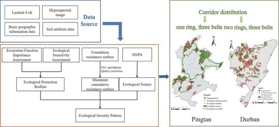
Remotesensing 13 02865 g001
Figure 2. Flow chart of ecological protection redline delimitation.
Remotesensing 13 02865 g002
Figure 3. Evaluation index of ecosystem service function. (a) Soil erosion results of Pingtan. (b) Habitat quality results of Pingtan. (c) Carbon sequestration results of Pingtan. (d) Soil erosion results of Durban. (e) Habitat quality results of Durban. (f) Carbon sequestration results of Durban.
Remotesensing 13 02865 g003
Figure 4. Pingtan ecological sensitivity evaluation index.
Remotesensing 13 02865 g004
Figure 5. Durban ecological sensitivity evaluation index.
Remotesensing 13 02865 g005
Figure 6. Ecological sensitivity results. (a) Ecological sensitivity results of Pingtan. (b) Ecological sensitivity results of Durban.
Remotesensing 13 02865 g006
Figure 7. Pingtan Island Ecological redline. (a) Pingtan Island Ecological protection redline based on ecosystem service function. (b) Pingtan Island Ecological protection redline based on ecological sensitivity. (c) Pingtan Island Ecological redline.
Remotesensing 13 02865 g007
Figure 8. Durban Ecological redline. (a) Durban Ecological protection redline based on ecosystem service function. (b) Durban Ecological protection redline based on ecological sensitivity. (c) Durban Ecological redline.
Remotesensing 13 02865 g008
Figure 9. MSPA analysis results. (a) MSPA analysis results of Pingtan. (b) MSPA analysis results of Durban.
Remotesensing 13 02865 g009
Figure 10. Result of ecological sources extraction. (a) Result of ecological sources extraction of Pingtan. (b) Result of ecological sources extraction of Durban.
Remotesensing 13 02865 g010
Figure 11. Potential ecological corridors. (a) Potential ecological corridors of Pingtan. (b) Potential ecological corridors of Durban.
Remotesensing 13 02865 g011
Figure 12. Construction of ecological corridors. (a) Construction of ecological corridors of Pingtan. (b) Construction of ecological corridor of Durban.
Remotesensing 13 02865 g012
Figure 13. Results of Red-edge vegetation index. (a) Red-edge Normalized Difference Vegetation Index (NDVIred-edge) results of Pingtan. (b) Modified Red-edge Simple Ratio Index (MSRred-edge) results of Pingtan. (c) Chlorophyll Red-edge Index (CIred-edge) results of Pingtan. (d) novel Inverted Red-edge Chlorophyll Index (IRECI) of Pingtan.
Remotesensing 13 02865 g013aRemotesensing 13 02865 g013b
Figure 14. Vegetation index of the ecological source area.
Remotesensing 13 02865 g014
Figure 15. Ecological security pattern. (a) Ecological security pattern of Pingtan. (b) Ecological security pattern of Durban.
Remotesensing 13 02865 g015
Table 1. Data Sources.
DataStudy AreaYearResolutionData Source
Landsat 8 OLIPingtan201730 mGeospatial Data Cloud Platform (http://www.gscloud.cn/ (accessed on 25 January 2021))
Durban201730 mUnited States Geological Survey (https://earthexplorer.usgs.gov/ (accessed on 18 April 2021))
Zhuhai-1Pingtan202010 mProject team purchase (https://www.obtdata.com (accessed on 11 September 2020))
DEMPingtan201030 mGeospatial Data Cloud Platform (http://www.gscloud.cn/ (accessed on 25 January 2021))
Durban200030 mUnited States Geological Survey (https://earthexplorer.usgs.gov/ (accessed on 18 April 2021))
Soil DataPingtan——30 mNanjing Soil Research Institute (http://www.issas.ac.cn/ (accessed on 7 March 2021))
Durban——1 kmHarmonized World Soil Database (http://www.fao.org/ (accessed on 18 April 2021))
Geographic Information DataPingtan2017VectorNational Catalogue Service For Geographic Information (https://www.webmap.cn/ (accessed on 27 January 2021))
Durban2020VectorOpen Street Map(http://openstreetmap.org/ (accessed on 20 April 2021))
Table 2. Evaluation index system of Ecological Protection Redline.
Target Layer ACriterion Layer BIndex Layer CIndicator Meaning
Delimitation of ecological protection redlineImportance of ecosystem services B1Soil and water conservation function C1/t/hm2·aDifference between potential soil erosion and actual soil erosion
Carbon fixation and oxygen release C2/tCarbon storage calculated by carbon storage module of invest model
Biodiversity maintenance function C3Habitat index calculated by habitat quality module of invest model
Ecological sensitivity B2Elevation C4/mThe altitude of the evaluation unit
Slope C5Evaluate the steepness and slowness of surface units
Distance from railway C6/mInfluence degree of railway factors on the evaluation unit
Land-use type C7Land use mode of the evaluation unit
Distance from important waters C8/mThe distance between the evaluation unit and the important water area
Vegetation coverage C9Vegetation coverage of evaluation unit
Table 3. Grading standard and weight of ecological sensitivity assessment factors.
FactorWeightNot SensitiveMildly SensitiveModerately SensitiveHighly SensitiveExtremely Sensitive
12345
Elevation ×1/m0.08<5050–100100–200200–300>300
Slope ×2/°0.10<55–1010–1515–25>25
Distance to railway ×3/m0.05<500500–10001000–20002000–3000>3000
Land-use type ×40.24Build-up landUndeveloped landAgricultureGrasslandWater body; Forest land
Distance to important water area ×5/m0.18>500300–500100–30050–100<50
Fractional Vegetation coverage ×60.10<0.180.18–0.390.39–0.620.62–0.82>0.82
Habitat Quality ×70.25<0.10.1–0.30.3–0.70.7–0.95>0.95
Table 4. Relative resistance coefficient of species movement.
Land Use TypeRelative Drag (R0)
Forest land1
Grassland50
Build-up land500
Water body10
Agriculture; Undeveloped land100
Table 5. Red-edge Vegetation Indices and calculation formulas.
IndexFormulaCorresponding Bands of Zhuhai-1 SatelliteDescribe
NDVIred-edge ( ρ 750 ρ 705 ) / ( ρ 750 + ρ 705 ) b19, b16Red-edge Normalized Difference Vegetation Index (NDVIred-edge). The valley and peak with red-edge are used to replace the NIR and Red band in traditional NDVI. It is related to leaf area index and chlorophyll content [44].
MSRred-edge ( ρ 750 ρ 445 ) / ( ρ 705 + ρ 445 ) b19, b16, b1Modified Red-edge Simple Ratio Index. It corrects the reflection effect of leaves and can be used to monitor the growth of vegetation canopy [45].
CIred-edge ( ρ 750 800 / ρ 690 725 ) 1 b19, b15Chlorophyll Red-edge Index. It shows a significant linear relationship with chlorophyll and nitrogen content [46].
IRECI ( ρ 783 ρ 665 ) / ( ρ 705 / ρ 740 ) b22, b13, b16, b19Novel Inverted Red-edge Chlorophyll Index. It has a good correlation with the chlorophyll content of plant canopy, which can be used to characterize the chlorophyll content of plants [47].
Table 6. Statistics of ecologically sensitive area.
Sensitivity LevelPingtanDurban
Area (km2)Proportion (%)Area (km2)Proportion (%)
Insensitive area79.9328.04322.6214.24
Low sensitive area78.3727.69567.0625.03
Moderately sensitive area53.8618.89483.5521.34
Highly sensitive area42.2614.82480.6621.22
Extremely sensitive area30.6610.75411.5918.17
Table 7. Statistics of different landscape types.
Landscape TypePingtanDurban
Area (km2)Proportion of Landscape in Prospect (%)Area (km2)Proportion of Landscape in Prospect (%)
Core Area43.1151.54286.4253.66
Islet6.377.6261.4711.51
Perforation2.12.519.561.79
Edge Area18.6922.350.080.01
Loop2.332.7820.123.77
Bridge3.994.7766.0812.38
Branch7.058.4390.0716.87
Table 8. Patch importance matrix based on Gravity Model of Pingtan.
Plaque Number123456789101112131415
11.34.03.82.7585.470.169.327.817.96.93.84.34.74.6
26.10.60.51.51.93.01.50.91.00.60.70.70.7
343,914.332.45.84.47.23.613.02.215.017.919.818.5
432.55.54.16.73.412.22.114.817.619.518.2
53.72.94.62.36.71.5109.3129.1157.3122.8
646.450.321.033.16.45.46.26.76.6
72015.9420.620.618.24.14.75.15.0
84175.323.635.56.77.78.38.1
910.120.93.43.84.14.0
103.712.113.214.613.7
11 2.12.42.52.5
125290.623,988.62850.4
1319,346.816,312.4
147155.7
15
Table 9. Area proportion of land-use types with different corridor widths of Pingtan.
Land Use TypesCorridor Width (m)
50100200300400
Forest land0.580.550.540.540.54
Grassland0.050.060.060.060.06
Agriculture0.120.140.160.170.17
Undeveloped land0.040.040.040.040.04
Water body0.120.100.090.080.07
Build-up land0.090.100.110.120.13
Table 10. Patch importance matrix based on Gravity Model of Durban.
Plaque Number12345678910111213141516
113.516.45.9395.5311.8629.11642.471.3147.7150.9553.484.174.214.746.5
25.622.110.815.422.418.89.829.719.131.927.685.96.260.5
34.318.431.120.917.010.226.525.421.418.214.48.511.0
45.47.29.77.55.311.68.111.99.516.911.813.4
5405.6189.8240.642.1124.1185.0181.277.746.416.631.1
6187.5224.345.0475.41500.1180.5266.376.830.349.5
71449.6314.5253.2118.4996.5143.4125.618.378.3
840.4155.734.0116.437.537.18.525.7
960.734.5118.338.137.78.626.1
10364.9627.6290.4211.828.2122.7
11129.0598.8111.643.268.7
12332.7252.419.6141.4
13275.525.5142.4
1431.1174.0
152814.7
16
Table 11. Area proportion of land-use types with different corridor widths of Durban.
Land Use TypesCorridor Width (m)
1002004008001200
Forest land67.7663.2258.3953.8750.41
Grassland1.521.722.032.732.89
Agriculture10.6012.9416.8121.3225.08
Undeveloped land10.6010.339.187.936.95
Water body0.030.070.130.160.19
Build-up land9.4911.7213.4713.9914.49
Table 12. Mean value of vegetation index of different land types.
Land Use TypesNDVIrgMSRrgCIrgIRECI
Undeveloped land0.380.260.100.09
Water body0.510.370.130.11
Build-up land0.340.220.080.07
Grassland0.500.350.160.14
Agriculture0.400.270.120.10
Forest land0.610.460.240.18
Table 13. Mean value of Vegetation Index in different ecological sources.
Ecological SourceNDVIrgMSRrgCIrgIRECIVIs
10.250.480.250.160.28
30.220.410.220.170.25
40.210.430.210.170.26
50.220.430.220.170.26
60.280.500.280.200.31
70.260.530.260.180.31
80.290.500.290.210.33
90.230.430.230.180.26
100.240.520.240.160.29
110.240.430.240.170.27
120.420.680.420.270.45
130.350.580.350.220.37
140.310.530.310.210.34
150.330.540.330.220.36
Publisher’s Note: MDPI stays neutral with regard to jurisdictional claims in published maps and institutional affiliations.

