
Snow Cover Variability in the Greater Alpine Region in the MODIS Era (2000–2019)


Department of Environmental Science and Policy, Università degli studi di Milano, Via Celoria 2, 20139 Milano, Italy
*
Author to whom correspondence should be addressed.
Remote Sens. 2021, 13(15), 2945; https://doi.org/10.3390/rs13152945
Submission received: 14 June 2021
/
Revised: 16 July 2021
/
Accepted: 23 July 2021
/
Published: 27 July 2021
(This article belongs to the Special Issue Recent Advances in Cryospheric Sciences)
Abstract
:Snow cover is particularly important in the Alps for tourism and the production of hydroelectric energy. In this study, we investigate the spatiotemporal variability in three snow cover metrics, i.e., the length of season (LOS), start of season (SOS) and end of season (EOS), obtained by gap-filling of MOD10A1 and MYD10A1, daily snow cover products of MODIS (Moderate-resolution Imaging Spectroradiometer). We analyze the period 2000–2019, evaluate snow cover patterns in the greater Alpine region (GAR) as a whole and further subdivide it into four subregions based on geographical and climate divides to investigate the drivers of local variability. We found differences both in space and time, with the northeastern region having generally the highest LOS (74 ± 4 days), compared to the southern regions, which exhibit a much shorter snow duration (48/49 ± 2 days). Spatially, the variability in LOS and the other metrics is clearly related to elevation (r2 = 0.85 for the LOS), while other topographic (slope, aspect and shading) and geographic variables (latitude and longitude) play a less important role at the MODIS scale. A high interannual variability was also observed from 2000 to 2019, as the average LOS in the GAR ranged between 41 and 85 days. As a result of high variability, no significant trends in snow cover metrics were seen over the GAR when considering all grid cells. Considering 500-m elevation bands and subregions, as well as individual grid points, we observed significant negative trends above 3000 m a.s.l., with an average of −17 days per decade. While some trends appeared to be caused by glacierized areas, removing grid cells covered by glaciers leads to an even higher frequency of grid cells with significant trends above 3000 m a.s.l., reaching 100% at 4000 m a.s.l. Trends are however to be considered with caution because of the limited length of the observation period.
1. Introduction
Snow cover is an essential parameter in the Earth’s energy budget and hydrological cycle. It has a large-scale cooling effect modulating the albedo of our planet and reflecting solar radiation back into space [1]. It provides a significant contribution to runoff in many populated areas of the world, where it represents a primary source of drinking water [2] and supports irrigation, the industry and energy production [3]. It helps feeding and preserving glaciers [4] and insulates the soil, influencing the thermal regime of permafrost, its distribution and properties [5]. Snow cover phenology further modulates habitat interactions of several plant and animal species [6,7,8], and changes in the seasonality of snow cover in high mountain ecosystems might put the survival of some species at risk [9,10]. In the European Alps, meltwater from snow cover makes up a consistent share of runoff used for hydropower generation [11,12]; snow also plays a vital role for the economy of the Alpine region by supporting winter tourism through skiing and other winter sports [4,13]. These activities are, in fact, dependent on the snow depth and distribution, and they are severely affected by the current climate change, which can lead to a reduction in snow cover as the increasing air temperature leads to more precipitation falling as rain and earlier snowmelt in the spring [14]. Moreover, snow may cause natural disasters such as avalanches or floods as a consequence of the melting process [15,16].
Across the Alps, changes in the duration, onset and melt-out dates of snow cover have already been observed at several locations from in-situ weather station records: Valt and Cianfarra [17] reported a decrease in winter and spring snow cover durations since the 1950s at a rate between 0.4 and 5 days per decade from stations located in the eastern and western Italian Alps, while Bocchiola and Diolaiuti [18] observed negative trends in the snow depth starting in the 1990s from a record of 40 stations located in the Adamello region. In the French Alps, a decrease in the average snow depth of −39 cm between 1960 and 1990 and 1990 and 2017 was reported by Lejeune et al. [19] at Col de Porte (1325 m a.s.l.); in Switzerland, a step like decrease in snow days between 20% and 60% since the end of the 1980s was observed by Marty [20], while in Austria, a decrease in the winter snow cover duration between 1980 and 2000 compared to 1896–1916 was found significant at stations in the southern region of the country [13]. The negative trend in Alpine snow cover duration was further confirmed by Matiu et al. [21] on the basis of an analysis of more than 800 station records from 1971 to the present.
While ground stations are able to provide snow cover observations up to the 1950s, or even to the 1900s [13], the data are sparse, often incomplete and representative only of a small area around the point of measurement, which can affect the assessment of long term trends and lead to issues if the snow cover data are to be used for the estimation of runoff and for projecting future changes in the freshwater availability of river systems [22]. Satellite records are thus often used to complement or substitute in-situ observations: the snow cover duration in the Northern hemisphere since 1967 is, for instance, available from a combination of satellites through the NOAA (National Oceanic and Atmospheric Administration) snow cover extent climate data record; however, the coarse resolution of this product (approximately 200 km) and its binary snow grid make it difficult to observe trends in mountain regions [3]. Observations from the AVHRR (Advanced Very-High-Resolution Radiometer) sensor available from a suite of NOAA satellites have also been used to estimate the snow cover variability since the mid-1980s, e.g., in the Alps [23] and Central Asia [24] at a 1-km spatial resolution, but the processing of AVHRR data in the early period is complicated by a lack of scenes and the presence of only one thermal channel for discrimination between snow and clouds [24], which limit its applicability. The sensor that has showed the greatest potential for snow cover studies is, in fact, MODIS (Moderate-resolution Imaging Spectroradiometer). Compared to AVHRR, MODIS benefits from a finer spatial resolution (500 m) and the availability of validated snow cover products such as MOD10A1 [25], and although it has a shorter period of data coverage (since 2000), it has now reached 20 years in orbit, building an invaluable data record and approaching the minimum time required for climatological analysis. Several studies have employed MODIS, based on either the daily or the 8-day product, to investigate the spatial distribution and interannual variability in snow cover at the regional scale and to estimate the runoff characteristics [16,26,27]. Some studies have also included the Alps as part of a larger area: for instance, Dietz et al. [28] observed snow cover characteristics in Europe from 2000 to 2011, while Notarnicola et al. [29] investigated snow cover changes over major mountain chains of the planet from 2000 to 2018. However, a detailed investigation of the spatial patterns of snow cover, temporal changes and their drivers in the Alps using the most recent MODIS observations is lacking. In this study, we focus on the Greater Alpine Region (GAR) and use MODIS data from 2000 to 2019 to investigate patterns of snow cover variability in space and time.
After the Introduction (Section 1), the presentation of the Study area (Section 2.1), Data (Section 2.2) and the Methods adopted for the analysis (Section 2.3 and Section 2.4), we (1) describe the spatial patterns in snow cover onset, duration and melt-out (Section 3.1); (2) investigate the influence of topographic and geographic variables as drivers of snow cover variability (Section 3.2) and (3) examine the interannual variability and trends in snow cover metrics from 2000 to 2019 (Section 3.3). Then, the results are discussed in Section 4, and finally, some conclusive remarks are given in Section 5.
2. Materials and Methods
2.1. Study Area
The GAR is defined in this study as the area between 4 and 19°E longitude, 43 and 49°N latitude, as in the HISTALP (Historical Instrumental Climatological Surface Time Series Of The Greater Alpine Region) grid [30]. We further identified four subregions to investigate the spatial variability of the snow cover and its links to the topographic and geographic variables by splitting the GAR along a geographic north–south and east–west divide. The north–south division follows the main topographic divide of the Alpine chain, running along the border between Italy to the south and Austria/Switzerland to the north; west of the Alpine chain, the division follows the divide between the basin of the Rhone River and the rivers flowing directly into the Mediterranean Sea, while, to the east, the line follows the divide between the basin of the Danube River and the rivers flowing into the Adriatic Sea. The east–west divide is also based on European river basins. North of Italy, the separation follows the divide between the Rhine and Danube River basins. In Italy, the line follows the divide between the Po and Adige basins, then Po and Reno and Arno and Tevere (see Figure 1). While previous studies have used dimensionality reduction techniques for the identification of subregions [21,30], we chose river-based divisions in this study, as the snow cover variability has important implications for the freshwater availability of river systems. The climate of the GAR is rather diverse, ranging from maritime influences from the Mediterranean Sea and the Atlantic Ocean to continental features in the Eastern European plains and inner Alpine valleys [30]. The Alpine region has experienced over the past several decades a significantly higher temperature trend than the Earth’s average, with the HISTALP database reporting a temperature increase of about 1.5 °C in the past 150 years both in low- and high-elevation areas [30]. Additionally, precipitation variability and changes in its seasonality have been documented [31]. In contrast, in this area, the emission of pollutants has strongly decreased over the past decades, causing a significant trend in all variables connected to atmospheric transparency, with the only exception of high-level areas that fall outside the atmospheric layer directly influenced by ground-based pollutant emissions [32,33]. The average elevation of the area is slightly above 600 m, with areas above 1000 m making up 19% of the total (see Figure 1). The elevation is not uniform across the four subregions: the southeastern region has the highest mean elevation (723 m a.s.l.), while the southwestern has the lowest (493 m a.s.l.), with a frequency peak around 280–300 m a.s.l. The northwestern region features a frequency peak around 480–500 m a.s.l.
2.2. Snow Cover and Ancillary Data
To identify snow-covered pixels in the GAR, we employed data from the MOD10A1 and MYD10A1 products, generated by the US National Snow and Ice Data Center (NSIDC), at a 500-m resolution [34]. All scenes from 2000 to 2019 were automatically downloaded and subset to the GAR domain using the Google Earth Engine platform (https://developers.google.com/earth-engine/datasets/catalog/MODIS_006_MOD10A1, last accessed on 26 July 2021 and https://developers.google.com/earth-engine/datasets/catalog/MODIS_006_MYD10A1, last accessed on 26 July 2021). MOD10A1 scenes are processed from the data acquired by MODIS onboard Terra platform, with a morning overpass (approximately 10:30 a.m. at the equator), while MYD10A1 is generated from the radiance acquired by MODIS onboard the AQUA platform, cycling the Earth on an afternoon overpass (approximately 1:30 p.m. at the equator). The basis of snow classification is the normalized difference snow index (NDSI), which uses reflected solar radiation in the visible (band 4, 0.545–0.565 μm) and shortwave infrared (band 6, 1.628–1.672 μm for MODIS Terra; band 7, 2.105–2.155 μm for MODIS Aqua) bands (see Equation (1) for MODIS Terra; the one for MODIS Aqua uses band 7 in place of band 6) to increase the contrast between snow-covered and snow-free surfaces [25].
Data screening is carried out to remove uncertain snow detections, while clouds are masked using a combination of tests based on visible, shortwave and longwave infrared channels [35,36]. In this study, we used the daily albedo grid of MOD10A1 and MYD10A1 products, which, for each grid point, provides a combination of scene classification (snow, land, water or cloud) and an albedo value for snow. Grid values 1–100 are reserved for snow/ice with its corresponding albedo (in percentage), while land surfaces are classified as 125, water and ocean as 137 and 139, respectively, and cloud as 150. Other values represent error conditions [34]. To mask water pixels (lakes, rivers and sea), we used the MODIS land cover product MCD12Q1, which includes several classification schemes, to discriminate between land cover types on a yearly basis. We employed the classification from the Annual International Geosphere-Biosphere Programme in a conservative way, so that grid points classified as water in any year were masked in our analysis.
We further obtained the elevation of the grid points from the ALOS (Advanced Land Observing Satellite) Global Digital Surface Model “ALOS World 3D-30m (AW3D30)” Digital Elevation Model [37] for the entire study area with a resolution of 30 m and resampled the Digital Elevation Model (DEM) to 500 m for consistency with the MODIS products. From the resampled DEM, we derived the slope and aspect to analyze the contribution of the topography to the variability in snow cover. We also calculated the shading index based on the number of hours a grid point lies in topographic shadow over a year. A grid point theoretically receiving solar radiation 24 h a day 365 days a year would have a shading index of 0, while a grid point that is always in shadow would have a shading index of 1. Topographic shading was calculated based on the procedure described by Senese et al. [38]. We also extracted the latitude and longitude of each pixel using the grid centroid. Data processing was carried out in a MATLAB environment and ArcGIS Pro 2.7.
2.3. Cloud Cover and Gap Filtering
While MODIS snow products provide observations on a daily basis, the presence of cloud cover can lower the data availability in the study area; as with data in the spectral range of visible radiation, it is impossible to observe the surface beneath clouds. Cloud cover can be rather high in the Alpine region: in the winter, low clouds can form in the valleys and persist for several days, while in the summer, the Alpine ridge features local spots of high cloud cover caused by convection. As a result, the 5-year mean cloud cover over the GAR can exceed 80% [39]. A number of different approaches have been proposed to filter cloud cover data and reveal the value of the grid points underneath, mostly based on a combination of spatial and temporal filters [40,41,42]. In this study, we adapted the method proposed by Gafurov and Bárdossy [43]. To apply cloud cover filtering, we first reclassified each MOD10A1 and MYD10A1 scene to obtain three surface classes: snow-covered, snow-free and cloud-covered. Thus, the grid values between 1 and 100 were reclassified as snow-covered (with a value of 1); land, ocean and water were reclassified as snow-free areas (with a value of 0), while cloud cover was reclassified to −1. Error values were also reclassified as cloud cover for the purpose of filtering. Additionally, a few gaps in data acquisition occurred in the early years of MODIS; we treated these days as grids with 100% cloud cover. Note that we chose to include all grid points classified as snow by MOD10A1 and MYD10A1, which might also include those that are only partly snow-covered and permanent ice.
The approach by Gafurov and Bárdossy [43] followed a series of steps by combining Terra and Aqua products and applying different temporal and spatial filters to obtain a binary grid where each point was reclassified as either snow-covered or snow-free. The steps are briefly summarized:
- Step 1: Combination of MOD10A1 and MYD10A1 products. By taking advantage of the different overpass time of Terra and Aqua satellites and the movement of clouds in between, the surfaces beneath clouds can be partly revealed. Let MODi,j,t be the snow cover grid point of the MOD10A1 product at each date t for grid row i and column j and MYDi,j,t the corresponding value of MYD10A1 for the same date and grid location. This step assumes that no snowmelt or snowfall occurred during the overpass of the two satellites on the same day. Snow cover from the MOD10A1 product forms the basis of the snow grid used in further processing steps, as this product is considered more accurate than its counterpart obtained from Aqua observations [44]. Thus, if MODi,j,t is cloud-free, the combination grid Si,j,t will retain its value, while if MODi,j,t is covered by clouds, Si,j,t will use the value of the MYDi,j,t grid point, i.e.,
This step has been applicable since the launch of the Aqua satellite in 2002; before this date, the MOD10A1 product was used without changes.
- Step 2: Temporal combination of adjacent dates. Cloud cover can vary greatly from one day to the other. Thus, a combination of snow cover data from adjacent dates can be used to infer the presence of snow on a cloud-covered date, assuming that no snowmelt or snowfall occurred on the adjacent dates. For each grid point Si,j at date t, the grids at date t − 1 and t + 1 are considered. If a grid point is snow-covered on both dates, Si,j,t becomes snow-covered. The same occurs for snow-free pixels. If the surface conditions on date t − 1 and t + 1 are different, the pixel is left unchanged.
If the grid point remains cloud-covered after the first iteration, a further combination of dates ((t − 1, t + 2) and (t − 2, t + 1)) is also considered to slightly extend the interpolation period while keeping a reasonable assumption that no snowmelt or snowfall processes occur. Thus, if a pixel remained cloud-covered after the application of Equation (3), Equation (4) was also applied.
- Step 3: Calculation of the snow transition elevation. This step is based on finding the snow cover elevation range on a certain date. For each date t, the elevation of the maximum snowline (above which all pixels are snow-covered) and minimum snowline (elevation below which all pixels are snow-free) are calculated. This step then assumes that no snow should be found in cloudy pixels below the minimum snowline and that all cloudy pixels above the maximum snowline should be covered by snow. A grid point is then reclassified as snow if its elevation Hi,j is higher than the maximum snowline and as snow-free if its elevation is lower than the minimum snowline, following Equation (5):
This step is only applied if the total cloud cover in the GAR on date t does not exceed 30%, as suggested by Gafurov and Bárdossy [43], because it might otherwise lead to an incorrect estimate of the snowlines and introduce large errors.
- Step 4: Spatial interpolation. In this step, a plus sign-shaped neighborhood of four points around each grid point is considered (i.e., points Si−1,j, Si+1,j, Si,j−1 and Si,j+1). If at least 3 out of four of these points are snow-covered (snow-free), the grid point is reclassified as snow-covered (snow-free). The assumption of this point is based on spatial autocorrelation, so that the middle grid point will, with high probability, have the same surface type as the nearby grid points.
- Step 5: Combination of snowline elevation and spatial interpolation. In this step, the 3 × 3 neighborhood of each grid point is examined, and the elevation and snow cover of each non-cloudy pixel is considered; the central point is reclassified as snow-covered if any of the neighboring points is snow-covered and its elevation is lower than that of the central point, i.e.,
This step is based on the decrease in temperature with increasing elevation; thus, snow on adjacent grid points lying at a higher elevation should melt later compared to grid points at a lower elevation.
- Step 6: Temporal combination. In the final step, we iteratively consider the subsequent dates for all points that have remained cloud covered after the application of steps 1–5. For each grid point, dates (t + 1, …, t + n) are considered until a date is found where the point Si,j,t+n is snow-covered or snow-free. The value of the grid point on date t + n is then assigned to grid point Si,j,t. This step might introduce the largest uncertainty, since it assumes no snowfall or snowmelt occurred during the interpolation period, which might not necessarily be true if the number of cloud-covered days is large.
2.4. Calculation of Snow Cover Metrics (Length, Start and End of the Snow Season)
Three metrics (length, start and end of the snow season) were used to describe the spatial and temporal patterns of the snow cover variability in this study. The metrics are based on the calculations of the snow cover duration for each grid point over a fixed period. The length of the snow season (LOS) is defined as the number of days of snow cover in a hydrological year, i.e., from 1 October to 30 September of the following year, following Equation (7).
where k is the day of the hydrological year, ranging between 1 and 365 or 366 for leap years. We defined the start and end of the snow cover season based on the fixed-date method described in the work by Wang and Xie [45]. The start of the snow season (SOS) is defined with respect to the number of snow cover days between the 1st of October and the 25th of January, which was found as the day with the highest snow cover on average in the GAR considering all years.
Here, D is the number of days from the start of the hydrological year to the 25th of January; the snow cover duration is also summed up from 1 October to 25 January. Lastly, we defined the end of the snow season (EOS) with respect to the number of snow days between the 25th of January and the 30th of September as:
Here, D is the number of days from the start of the hydrological year to the 25th of January, and the snow cover duration is summed up from the 25th of January to the 30th of September. This method thus does not consider transient snowfall and melt-out events, which would require the definition of multiple start and end dates, or the choice of a threshold of days to filter these events out, as in Notarnicola [29]. In areas of low elevation, the SOS and EOS do not reflect a continuous snow period but, rather, the number of snow cover days in the early part of the hydrological year (SOS, before the 25th of January) and late part of the hydrological year (EOS, between the 25th of January and 30th of September). For high elevation regions, where snow cover is reasonably continuous, the correspondence between the day of the hydrological year and date is reported in Table 1 for each 15-day period.
For each of the three metrics, we calculated the trends over the period 2000–2018 (corresponding to hydrological years 2000 to 2001 and 2018 to 2019). The significance of the trends was evaluated using the nonparametric Mann–Kendall test [46], which is used to identify monotonic (but not necessarily linear) trends in a time series. We calculated the slope and intercept of the trends using the Theil-Sen estimator [47] which is more robust to outliers compared to ordinary least-squares linear regression.
3. Results
3.1. Means of Snow Cover Metrics over the GAR
Along the Alpine chain, at elevations between 1500 and 3000 m a.s.l., the average snow duration (LOS) over the 2000–2019 period was 202 ± 3 days. This value was obtained when calculating the mean LOS value over all the grid points in this elevation interval (bright green pixels in Figure 2a—the mean elevation of these grid points is 2050 m a.s.l.) for every year and then performing the mean over the 20-year period, while the uncertainty was expressed as the standard error of the 20-year mean. The highest values were found for glaciers, whose average LOS was 360 ± 4 days (blue pixels in Figure 2a). The very high LOS values of glaciers depend on the fact that, for them, the snow period is often very long but, also, from the fact that MODIS does not distinguish between snow-covered and snow-free glaciers. The other mountain regions in the GAR outside the main Alpine chain, i.e., the Jura, Vosges, Black forest, Bavarian forest, Dinaric Alps, Cevennes and Apennines, with elevations between 1000 and 1500 m a.s.l., also showed a high average LOS, with a value of 106 ± 4 days (see yellow pixels in Figure 2a). In contrast, low-lying areas (elevations lower than 500 m a.s.l.) south of the Alps, such as the Po plain and the mouth of the Rhone in Southern France, located in the southwestern (SW) region, had an average LOS under 10 days (red pixels in Figure 2a). However, in these areas, the LOS does often not reflect a continuous snow cover period but only the number of snow cover days over an entire year.
Aside from the Po plain and the mouth of the Rhone area, a slightly higher duration of the snow season was observed in the other low elevation areas in the GAR. This is the case of the eastern side of the Alps, particularly in the northeastern (NE) region, which had the highest average LOS for grid points with elevations lower than 500 m a.s.l. (45 ± 4 days) and at all elevations (74 ± 4 days). The snow cover duration was also relatively high in the northwestern (NW) region (60 ± 2 days considering all grid points and 25 ± 2 days for elevations lower than 500 m a.s.l.), while the southeastern (SE) and SW region had very similar values, with 49 ± 2 days for all points, 11 ± 1 days at elevations <500 m a.s.l. in the SE region compared to 48 ± 2 days at all elevations and 13 ± 2 days at elevations <500 m a.s.l. in the SW region.
The start of the snow season (SOS) was, on average, around day 33 ± 2 of the hydrological year at elevations between 1500 and 3000 m a.s.l. of the Alpine chain (see bright green pixels in Figure 2b), day 63 ± 2 of the hydrological year for the other mountain regions in the GAR at elevations between 1000 and 1500 m a.s.l. and gradually earlier for higher-relief areas (day 3 of the hydrological year on average at elevations >3000 m a.s.l.; see the blue pixels in Figure 2b). In contrast, in low-relief areas (elevation <500 m a.s.l.), the SOS started, on average, on day 97 ± 2 of the hydrological year (orange pixels in Figure 2b), even if, in these areas, SOS does often not correspond to the start of a continuous snow cover period. As observed with the LOS, the NE region showed the earliest SOS on average considering all elevations (day 76 ± 2 of the hydrological year, compared to 86 ± 1 for the NW region, 92 ± 1 for the SE region and 93 ± 1 for the SW region, which includes the Po plain).
The end of season (EOS) generally occurred around day 235 ± 2 of the hydrological year at elevations between 1500 and 3000 m a.s.l. of the Alpine chain and day 169 ± 2 of the hydrological year for the other massifs in the GAR at elevations between 1000 and 1500 m a.s.l. (yellow pixels in Figure 2c). Above 3000 m a.s.l., the EOS occurred, on average, on day 346 ± 1 of the hydrological year, while, at elevations below 500 m a.s.l., such as across the Po plain and in the mouth of the Rhone area, the average EOS occurred on day 128 ± 2 of the hydrological year (red pixels in Figure 2c). Additionally, in this case, at low elevations, the EOS does often not correspond to the end of a continuous snow cover period. For the EOS, a slightly later value was observed for the NE region (day 150 ± 3 of the hydrological year compared to day 145 ± 1 of the hydrological year in the NW region). In the SE region, snow disappeared earlier than in all other regions (average EOS: day 141 ± 1 of the hydrological year in the SE region and 142 ± 1 in the SW region).
3.2. Factors Explaining the Spatial Variability in the Snow Cover
The main geographical variable determining the LOS is elevation. The strong relationship between LOS and elevation is evident from Figure 3, where we represented, for each 5-m interval of the elevation range of the GAR, several quantiles of the distribution of the corresponding LOS average values in the period 2000–2019. Considering the medians (violet points) of the distributions of the LOS values in the different 5-m elevation intervals, the relationship between LOS and elevation showed a very strong correlation between 1000 and 3000 m a.s.l. (Kendall’s Tau = 0.99). The same plot showed a similar behavior for different percentiles of the distributions of the LOS values in the 5-m elevation intervals, even if the range in which the relationship between the LOS percentile and elevation was linear changes among the percentiles. At an elevation about 100 m a.s.l., a jump in the average LOS occurred; this was caused by a number of lakes/rivers and humid areas that were not properly filtered by the water masks in MOD10A1/MYD10A1 and the additional mask from MCD12Q1 and were observed as snow-covered for up to 80 days by the MODIS snow products (see Figure 3).
Figure 3 also gives evidence that the values of LOS corresponding to a certain elevation have a large variability, with ranges often covering an interval larger than 100 days, suggesting that LOS depends not only on elevation but, also, on other climatic characteristics.
To highlight the rather wide range of LOS values corresponding to a given elevation, we represent in Figure 4 the difference between the average LOS of each grid point in the period 2000–2019 and the average LOS of all grid points falling in the same 5-m elevation interval.
The contrast between the grid points on the northern and southern sides of the Alps is striking; in the NE region, 91% of grid points have a higher LOS compared to those in their respective 5-m elevation range, whereas, in the NW region, the percentage of grid points with a higher LOS is much lower, 33%, owing to the inclusion of warm areas, e.g., in Southern France. In the SW and SE regions, 82% and 80% of the grid points have a lower snow duration compared to those at similar elevations. In contrast, the Po basin is rather homogeneous, with differences lower than 10 days (positive and negative) compared to areas at the same elevation. In Figure S1, we further represent the spatial distribution of the LOS grid point values, expressed in terms of the percentiles in the distribution of the GAR LOS values falling in the corresponding 5-m elevation intervals.
A clear distinction is evident between the points north of the Alps and south of the Alps, particularly in the NE region, where 82% of grid points have a percentile above the median and 46% above the 75th percentile, owing to the inclusion in this area of rather cold regions, such as the NE plains and the Balkan Peninsula north of the Danube River. In the NW region, 70% of the points have a percentile below the median, which is observed as a balance between the areas of Switzerland and Germany, with a larger number of points falling above the 50th percentile and a larger number of areas where the percentiles are lower the median, particularly in France towards the mouth of the Rhone. This latter pattern is also observed in the SW region, where 16% of grid points fall below the 5th percentile with respect to the elevation and 61% below the 25th percentile. In the SE region, an interesting difference is observed in the eastern part of Po basin north of the Apennine chain, where the LOS of the grid points is above the 75th percentile of the points located in the same elevation range (see Figure S1). Elsewhere in this region, most grid points fall below the median with respect to elevation: 10% below the 5th percentile and 53% below the 25th.
To investigate the geographic and topographic drivers of the snow cover variability in the GAR, we performed a linear regression on each metric using elevation, slope, aspect, shading, latitude and longitude as the independent variables. Latitude and longitude were included as the proxies for climatic variability in the area. This regression explains a high percentage of the variances in all three metrics, with the highest R2 for the LOS (0.91, see Table 2). Looking at individual variables, the most important factor overall is elevation, which alone explains up to 85% of the variability in the LOS and 86% in the EOS, while, for the SOS, a lower percentage of the variance is explained. The other variables appear less important. Moving from the GAR to the four subregions, the explained variance generally increases for all three metrics, with the LOS and the NW region having the highest R2 (0.94) and SOS in the NE region, the EOS in the SW region the lowest ones (0.89).
In order to better highlight the effect of these other variables, we considered the relation of the LOS, SOS and EOS with elevation, and we removed the effect of elevation from the data by subtracting the average value of the LOS, SOS and EOS in their respective 5-m elevation intervals. We subjected these residuals to the same multivariate analysis we performed for the LOS, SOS and EOS, obtaining an explained variance of 48%, 52% and 36%, respectively. Considering individual variables, latitude and longitude can explain most of the variance in the residuals of the three metrics, especially the SOS, with 32% of variance explained by latitude and 15% by longitude, while the two variables contribute to explaining 26% and 15% of the LOS. Neither aspect nor slope or shading can explain significant amounts of variance in these residuals in the GAR (max. 3% SOS explained by aspect), which indicates that the higher values we obtained for slope and for shading in Table 2 were actually caused by the fact that these variables have a significant correlation with elevation (Kendall’s Tau is 0.75 for aspect and 0.03 for slope, both significant at the 99% confidence level).
We then repeated the analysis concerning the residuals using 1000-m elevation ranges, as well as different LOS classes (LOS < 180 days, 180 < LOS < 330 and LOS > 330).
If we consider separate 1000-m elevation ranges, latitude appears to explain most of the residual variance, up to 34% for the LOS between 1000 and 2000 m a.s.l., and generally more for the SOS compared to the EOS and LOS (see Table 3); in general, the importance of all the variables tends to decrease with elevation, although there are some exceptions, e.g., aspect, which explains 18% of the variance in the SOS between 2000 and 3000 m a.s.l. As concerns slope, the variable explains a minimal amount of the variance, except for the EOS below 1000 m a.s.l., which might suggest a longer permanence of snow on sloping surfaces in this elevation band. Considering all variables in a multivariate regression, the maximum amount of explained variance is 57% for the SOS between 1000 and 2000 m a.s.l. Among the four subregions, the NW one shows the highest amount of explained variance between 1000 and 2000 m a.s.l. for all three metrics, ranging between 78% (SOS) and 68% (LOS) (see Table S1).
Considering the different LOS classes, a similar pattern was observed, as latitude explains most of the residual variance, up to 35% for the SOS for the grid points with the average LOS < 330 days (see Table 4), and the importance of the variables tends to decrease with the increasing average LOS. The multivariate regression showed a higher amount of explained variance below 180 days of the average LOS and the highest explained variance for the SOS (53%). Considering the different regions, the NW region is the one with the highest amount of residual variance explained below 180 days of the average LOS (58% in SOS), while the SE region is the one with the lowest amount (17% of the SOS for grid points with an average LOS < 180 days) (see Table S2).
3.3. Interannual Variability in Snow Cover Metrics and Trend Analysis
The standard deviations of the grid point LOS records in the 2000–2019 period (Figure 5a) show higher values (>20 days) for the high-relief areas on the southern side of the Alps, compared to the northern side. This is also highlighted when standardizing the standard deviation for elevation by subtracting the average standard deviation in 5-m elevation intervals (see Figure S2). The southern side of the Alpine chain thus shows a lower average LOS but a higher interannual variability (see Figure 4 and Figure S2). In contrast with high-relief areas, grid points located in low-relief areas in the southern regions (Balkan Peninsula, eastern Po basin and mouth of the Rhone) have a generally low standard deviation (<10 days), although this is often caused by the fact that the LOS of these points is 0 over multiple years. The lowest values are those of glaciers, whose standard deviation is generally close to 0. Compared to the plains south of the Alps, the northern ones generally have LOS grid point records with larger standard deviations, and the NE region shows the highest average standard deviation of the LOS records of 24 days, whereas, in the other regions, the average standard deviation of the LOS records is rather similar, ranging between 16 and 17 days.
Besides the standard deviation of the LOS grid point records, it is also interesting to present the ratios between these values and the corresponding average values (Figure 5b), which shows rather high values in many areas, as 4% of the pixels have higher LOS standard deviations than the LOS average. The errors of the average LOS grid point values are indeed lower because of the averaging over the 20-year period. However, these rather high values suggest that a LOS climatology with a 20-year period of observations might still have some uncertainty caused by the high year-to-year variability of the LOS grid point records. This problem particularly concerns low-elevation areas that often do not have a continuous snow cover period.
In order to complete the presentation of the standard deviations of the grid-point LOS records, we present in Figure 5c several quantiles of the distribution of the grid point ratios between the LOS standard deviations and LOS mean values in each 5-m interval of the GAR elevation range. Here, a decrease in this ratio is evident with the increasing elevation, with values above 1 for the 99th percentile of the distribution of the ratio below 1000 m a.s.l. and all percentiles nearing 0 above 2500 m a.s.l., indicating a higher and important role of the interannual variability of the LOS records on the ratios at low elevations than at high elevations. The figure also shows the same jump at elevations about 100 m a.s.l. observed in Figure 3, which appears to be caused by the erroneous classification of some water bodies.
We further examined the interannual variability of the snow cover metrics over the period of investigation, 2000–2019, by calculating the average of the different snow cover metrics for each year over the GAR and considering the individual regions and elevation bands. In the GAR, a high year-to-year variability was observed in the LOS, ranging from 41 days in 2006 to 85 days in 2005 (see Figure 6). Considering the four subregions, the NE region always showed the highest LOS, ranging between 43 and 110 days, while the SW and SE had the lowest (32–67 days). A similar high variability was observed for the SOS, which ranged over the GAR between day 72 of the hydrological year in 2010 and day 96 in 2006 (see Figure S3), and the EOS, which was observed to vary between day 134 of the hydrological year in 2001 and day 161 in 2004 (see Figure S4). No significant trends were observed for these metrics over the GAR, owing to the large interannual variability.
Considering the separate 500-m elevation bands, we observed that the lowest values of the LOS occurred nearly always in 2006 for all subregions and elevation bands below 3000 m a.s.l. (see Figure 6 and Figure 7). In contrast, years with above-average LOS were more heterogeneous among the subregions and elevations, with no prevalence of a specific year. An above-average LOS was observed for example in 2005 below 2000 m a.s.l. in the NE and SE regions, in 2012 between 1000 and 3000 m a.s.l. in most regions and in 2003 between 2000 and 3000 m a.sl. in all the subregions (see Figure 7). A high year-to-year variability was observed particularly below 500 m a.s.l., where the average LOS can range between 5 days (SW region in 2016) and 84 days (NE region in 2005) and between 1500 and 2000 m a.s.l., with a range of 87 days (SW region). The variability decreased with the elevation; between 3000 and 3500 m a.s.l., the LOS ranged between 316 days (SW region, 2017) and 359 days (NE region, 2000), while, above 4500 m a.s.l., the range was approximately 5 days in the NW region. Between 3000 and 4000 m a.s.l, significant trends at the 90% and 95% confidence levels were observed for the NW, NE and SW regions. Between 3000 and 3500 m a.s.l., the trends ranged between −5.4 and −6.3 days per decade, while the trends between 3500 and 4000 m a.s.l. were much lower in magnitude (see Table 5).
Compared to the LOS, a more heterogeneous pattern with respect to the years of maxima and minima was observed for the SOS and EOS (see Figures S5 and S6). In general, 2006 appeared as the year with the peak SOS for most regions and elevation bands in agreement with the low values found for the LOS, while 2003 and 2008 showed below-average SOS values. Significant positive trends (90–95% confidence level) for the SOS were observed between 3000 and 4000 m a.s.l. (with the only exception the SW region), ranging between +0.1 and +1.6 days per decade, with a greater magnitude in the lower elevation range, as for the LOS (see Table 5). For the EOS, 2006 and 2010 were observed as years with below-average values in most regions and elevation bands, while an above-average EOS was seen in 2012. No trends reached 90% significance for this metric, although most of them appeared negative above 2500 m a.s.l., while the opposite was true below this elevation (see Table 5).
To complete the analysis of the trends in the snow cover metrics, we also calculated them at the grid cell level. Among all grid points with significant trends, 91% showed negative trends (see Figure 8 and Figure 9), with an average of −17 days per decade, while a small peak in positive trends was observed around 4050 m a.s.l. Grid cells with trends significant at the 95% confidence level appeared concentrated mostly at elevations above 2500 m a.s.l., (77% of the total points with significant trends) because of the larger signal-to-noise ratio at the higher elevations (see Figure 5c). The fraction of the cells with significant trend peaks between 3000 and 3300 m a.s.l., where about 20% of the grid cells had negative trends. At higher elevations, the fraction of the cells with significant trends decreased, because a lower variability was observed, as most of the grid points had (near-) permanent snow cover throughout the period. At elevations below 2500 m a.s.l., the frequency of the grid points with significant trends was much lower, with an average fraction of 2%.
Spatially, grid cells with significant negative trends appeared distributed mostly in the NE areas, on the northern side of the Alps and in the Po basin, with values <−10 days decade−1. In contrast, a small number of significant positive trends (>5 days decade−1) were seen along the Dalmatian and Southern French coasts, the Apennine chain and in France at the northwest margin of the GAR (see Figure 9). The spatial patterns were similar for the SOS (see Figure S7), while, as seen in Table 5, the amount of pixels with significant trends was much lower for the EOS than for the other metrics. Significant negative trends in this metric were mostly found on the northern side of the Alps, as well as in the Po basin, while a small cluster of pixels with negative trends (<−5 days decade−1) was observed at the E margin of the GAR. Pixels with significant positive trends were instead observed on the Dalmatian and Southern French coasts (see Figure S8).
Thus, in low-elevation areas, particularly in the NE regions, the decrease in LOS appears to be caused by an increase in the SOS (>10 days decade−1) rather than a decrease in the EOS, which is of lower magnitude (see Figures S7 and S8).
4. Discussion
4.1. The Role of Glaciers
In the Alpine region, glaciers have been continuously retreating over the past decades, with a surface area loss rate of −1.2% year−1 [48]. As MODIS snow products do not directly distinguish between ice and snow, we evaluated the impact of glaciers on the observed trends in the snow cover metrics. To filter out glaciers, we used the Randolph glacier inventory version 6.0 (RGI, [49]), a global database of glacier outlines that includes outlines for the Alps from 2003. The outlines were rasterized to the same grid size of the MODIS snow products, and the fraction of glacier coverage in each cell was counted; we then filtered out the cells with varying fractions of glacier coverage.
The results of the filtering are shown in Figure 10. Grid cells that are entirely covered by RGI glaciers contribute very little to the trends in the LOS, and even lowering the coverage threshold to 80% makes up for a maximum of 3% of the significant trends in the elevation interval where the trend significance was highest (3000–3300 m a.s.l.). However, filtering out all grid cells that are glaciers covered by even a tiny fraction excludes most of the significant trends at elevations above 2500 m a.s.l. (see Figure 10a). Glacier cells with <80% coverage include the termini and frontal parts, which might have become snow-free compared to the outlines from the RGI but, also, other areas located at higher elevations away from the terminus (see Figure 10c,d). Here, trends in the LOS probably stem from an increase in debris cover/impurities, which lowers the number of cells seen as ice by the MODIS snow products over the years. This confirms observations by Azzoni et al. [50] and Fugazza et al. [51], who found an increase in debris cover and decreasing albedo for a mountain group in the Central Italian Alps.
In order to further investigate the role of glacierized areas on the frequency of grid cells with significant trends, we removed all glacier cells (i.e., all grid cells that were glacier covered by even a tiny fraction, regardless of the significance of their trends) from the database, and we recalculated the fraction of the grid cells with significant trends in each 50-m elevation interval: the frequency of the significant trends increased exponentially with elevations above 2500 m a.s.l., and at 4000 m a.s.l., all grid points outside the glaciers had significant negative trends, while only a few grid cells below 500 m a.s.l. showed significant positive trends. We thus also recalculated the significance and intensity of the trends by 500-m elevation bands when the glaciers were excluded. While little change was observed below 2500 m a.s.l., owing to the distribution of glaciers with elevations above 3500 m a.s.l., significant trends appeared in all the snow cover metrics in the GAR and in the SW region (except for the SOS between 3500 and 4000 m a.s.l., see Table 6); in the GAR, the magnitude of the trends suggests that the shortening of the LOS (−2.7 days decade−1 between 4000 and 4500 m a.s.l.) was mostly caused by earlier snow melt (−2.5 days decade−1 in the EOS). A higher magnitude of the EOS trends compared to the SOS was also observed for the NW and SW regions.
4.2. Snow Cover Variability in the Alps and Other Mountain Regions
While the focus of our analysis was the Alpine region from 2000 to 2019, other studies have investigated snow cover in the Alps either as part of a larger study or during different observation periods. We observed a high interannual variability in all snow cover metrics (LOS, SOS and EOS). Over the GAR, the longest LOS was observed in the hydrological year 2005/2006 (see Figure 6). This feature was also identified by Dietz et al. [28] in their study of European snow cover from 2000 to 2011 using MODIS. The event was attributed to high snowfall occurring in parts of Central Europe, including Austria, and was found to be particularly pronounced for lower elevation areas, below 1500 m a.s.l., mainly owing to a later EOS. In the GAR, we also identified the NE area as having the longest LOS in 2005/2006 below 1000 m a.s.l. (see Figure 7), while the southern regions did not show the same pronounced pattern.
In their study of snow cover in the Alpine region, Hüsler et al. [23] employed NOAA AVHRR data from 1991 to 2011. Their snow cover patterns broadly agreed with our findings, with the southern regions showing shorter LOS compared to the northern ones, particularly NE, and a strong relationship with height, which decreased at the higher elevations, suggesting the interplay of two factors: the temperature gradient with height controlled the LOS at lower elevations, while at the higher elevations, the importance of precipitation increased. Their analysis of extreme years also showed a shorter than average LOS during winter 2006/2007, in agreement with our analysis (see Figure 7), and an increased snow cover variability at lower elevations. We did not attempt to further correlate the snow cover metrics with meteorological variables, owing to the lack of a meteorological product at a comparable grid size to MODIS; in future research, this might be attempted using, e.g., high-resolution meteorological models or by the downscaling of global reanalysis products.
Compared to MODIS, NOAA AVHRR has the advantage of covering a larger timespan at the cost of a decreased spatial resolution, higher uncertainty and larger processing time. Nevertheless, its length of operation allows observing trends over longer time periods. Hüsler et al. [23] observed significant negative trends in the snow cover duration in the southern regions, generally below 1000 m a.s.l. In contrast, our LOS trends occurred mostly at higher elevations; the different periods of time analyzed and definitions of the subregions, as well as the importance of glaciers, appeared to play a role in these differences, and in fact, omitting glacier cells from our analysis also revealed significant trends in the SW region, although, again, at higher elevations compared to Hüsler et al. [23].
A further cause of differences might stem from the different snow algorithms and different spectral bands used by the two sensors, which might introduce variations in the classification of snowy pixels. In an attempt to solve this issue, Hori et al. [52] produced a combined snow cover record using the same approach on MODIS and AVHRR and analyzed the snow cover duration from 1982 to 2013 over the globe. A shortening of the LOS in Western Eurasia by two months over three decades was found, as well as a weak negative trend in the center of Siberia, Alaska and Eastern North America. However, no significant decrease was observed in the European Alps. In their study, a shorter LOS was associated with later snow onset dates as opposed to earlier melt. We performed a correlation analysis of our snow cover metrics and found that both the SOS and EOS correlated well with the LOS (average of 0.6 considering 1000-m elevation ranges and subregions), except above 3000 m a.s.l., where only the EOS was significantly correlated with the LOS, possibly indicating a larger importance of increasing temperatures, causing earlier snow melt at higher elevations. Weak negative trends in the Alps, albeit generally nonsignificant, were also found by Notarnicola [29], who analyzed the snow cover time series in the world’s mountain regions using the same MODIS snow cover product used in this study. Compared to the Alps, other regions such as Western Canada, Argentina and Chile showed much more negative trends in the LOS (<−20 days from 2000 to 2018), while, in the Grampian Mountains (UK), Northern Russia, Northern Africa, Australia and New Zealand, weak positive trends were found.
Before the 1980s, remote sensing data to evaluate the snow cover trends were scarce. Observations from in-situ stations that spanned the 1970s or earlier, however, tended to indicate a decreasing trend in snow cover duration in the Alpine region. Matiu et al. [21] observed negative trends below 2000 m a.s.l., more negative on the southern side (−7.0 days decade−1 between 1000 and 2000 m a s.l. and −4.8 days decade−1 below 1000 m a.s.l.), by analyzing more than 800 in-situ stations since 1971. A series of years with lower-than-average LOS was identified between the 1980s and 1990s, while little change has been observed since 2000, when MODIS started operating. [17,53,54]. Note, however, that very few stations are available above 3000 m a.s.l. [21]. To further confirm these long-term observations, it would be desirable to analyze the snow cover variability before the satellite era on a regular grid; this might be attempted in future research by spatializing station data using the approach of Gafurov et al. [55] or by employing reanalysis products such as ERA-5 [56], which has provided snow cover data since the 1950s by assimilating in-situ observations, although ERA-5 is known to overestimate the snow cover duration [57].
5. Conclusions
In this study, we used MODIS daily snow cover products to evaluate the variability in different snow cover metrics over the greater Alpine region (GAR) and four subregions based on geographic and climatic divides from 2000 to 2019. We found a high variability in the LOS both in space and time: the northern areas generally showed a higher LOS compared to the southern ones, considering all elevation ranges (74 ± 4 days in the NE region compared to 48 ± 2 in the SE and 49 ± 2 in the SW region), and high-elevation regions also showed higher snow cover durations compared to low-elevation ones. The LOS depended highly on elevation, with a very strong significant relationship between 1000 and 3000 m a.s.l. (correlation with median LOS is 0.99). Variability in the SOS and EOS was also explained by elevation, and similar patterns were seen compared to the LOS, as northern regions exhibited earlier snow cover onset (day 76 ± 2 of the hydrological year in the NE region compared to 93 ± 1 in the SW region) and later melt (day 150 ± 3 of the hydrological year in the NE region compared to 141 ± 1 in the SE region). Aside from elevation, other topographic variables such as slope, aspect and shading explained little variability in the snow cover metrics in the GAR, perhaps in view of the grid size of MODIS (500 m), while the geographic variables such as latitude and longitude had a slightly higher impact (maximum 0.34 R2 for latitude when regressing on residuals from the relationship with elevation). These results have implications for river flow modeling in the Alps and might lead to improved estimations of the peak discharge and water availability for hydropower energy production.
Interannually, the variability in the snow cover metrics was high particularly in the low-elevation regions, as exemplified by the ratio between the standard deviation of the LOS and its average, which decreased with the elevation. For this reason, a LOS climatology for low-elevation regions still suffered from uncertainty, and no significant trends were observed there; in contrast, for high-elevation regions (above 3000 m a.s.l.), the ratio between the standard deviation of the snow cover metrics and their average was lower, and this enabled building a snow cover climatology and assessing the trends. In fact, significant negative trends in the LOS and positive trends in the SOS were observed between 3000 and 4000 m a.s.l., with a decrease in the LOS of −5.2 days decade−1 in the GAR in the elevation range 3000–3500 m a.s.l. and a similar decrease in magnitude in the northern regions. We evaluated the effects of glaciers on these trends, as permanent ice is also included in MODIS snow cover products, and found that they contributed a large share of grid cells with significant trends above 3000 m a.s.l., e.g., 15% between 3000 and 3200 m.a.sl. When filtering out glacier cells altogether, however, we observed an increased frequency of significant trends above 2500 m a.s.l. and negative trends (95% confidence interval) in the LOS and EOS above 4000 m a.s.l. both in the GAR (−2.7 days decade−1 for the LOS and −2.5 days decade−1 for the EOS) and in the SW region (−5.6 days decade−1 for the LOS and −5.0 days decade−1 for the EOS). Thus, it appears that LOS trends in the northern regions above 4000 m a.s.l. are partly caused by retreating glaciers, while those in the southern ones might stem from increasing temperatures leading to earlier snow melt at high elevations. In contrast, in low-elevation regions, especially in the NE subregion, the decreasing LOS is linked to a later SOS, possibly caused by reduced snowfall, rather than an earlier EOS. Further research employing high-altitude station data or high-resolution/downscaled meteorological products would be necessary to confirm these trends over longer periods of time, which might lead to better predictions of snow cover permanence at high elevations under different climate change scenarios, with important consequences on the winter tourism sector and the economy of mountain regions.
Supplementary Materials
The following are available online at https://www.mdpi.com/article/10.3390/rs13152945/s1, Figure S1: Spatial distribution of the positions (expressed in terms of percentiles) of the LOS grid point values in the distributions of GAR LOS values falling in the corresponding 5-meter elevation intervals. Figure S2: Standard deviation of the LOS standardized by subtracting the average standard deviation of LOS in 5 m elevation intervals. Figure S3: Average Start of Season (SOS) over the GAR and four sub-regions. Figure S4: Average Start of Season (SOS) over the GAR and four sub-regions. Figure S5: Average Start of Season (SOS) over 2000–2019 in the four subregions of the Greater Alpine Region by elevation band. Figure S6: Average End of Season (EOS) over 2000–2019 in the four subregions of the Greater Alpine Region by elevation band. Figure S7: top panel: trend in the start of season (SOS) in days per decade in the Greater Alpine region from 2000 to 2019. Bottom panel: significance of trends in SOS over the GAR. Figure S8: top panel: trend in the end of season (EOS) in days per decade in the Greater Alpine region from 2000 to 2019. Bottom panel: significance of trends in EOS over the GAR. Table S1: Variance explained by linear regression of individual variables against the three metrics in the GAR for different elevation classes and sub-regions. Elevation is removed by subtracting the average in each 5 me elevation interval and a linear regression is applied to residuals. z represents elevation (m a.s.l.). Each cell reports the R2. Table S2: Variance explained by linear regression of individual variables against the three metrics in the GAR for different LOS (length of season) classes. Elevation is removed by subtracting the average in each 5 me elevation interval and a linear regression is applied to residuals. Each cell reports the R2.
Author Contributions
Conceptualization, D.F., V.M. and M.M.; methodology, D.F.; formal analysis, D.F., V.M. and M.M.; writing—original draft preparation, D.F., V.M., A.S. and M.M.; supervision, G.D. and M.M.; project administration, G.D. and M.M. and funding acquisition, G.D. and M.M. All authors have read and agreed to the published version of the manuscript.
Funding
This work was supported by Agroalimentare E Ricerca (Ager) under Grant 2017–1176 within the project IPCC-MOUPA (Interdisciplinary project for assessing current and expected Climate Change impacts onMOUntain Pastures). The researchers at UNIMI are also grateful to Sanpellegrino-Levissima S.P.A. for funding and support.
Data Availability Statement
All data used in this manuscript are freely available from online repositories. The MOD10A1 and MYD10A1 daily snow cover products are available from NSIDC at https://nsidc.org/data/mod10a1, last accessed on 26 July 2021 and https://nsidc.org/data/myd10a1, last accessed on 26 July 2021; MCD12Q1 are available from https://lpdaac.usgs.gov/products/mcd12q1v006/, last accessed on 26 July 2021 and the ALOS AW3D30 Digital Elevation Models are available after registration from https://www.eorc.jaxa.jp/ALOS/en/aw3d30/index.htm, last accessed on 26 July 2021.
Conflicts of Interest
The authors declare no conflict of interest.
References
- Flanner, M.; Shell, K.; Barlage, M.; Perovich, D.K.; Tschudi, M.A. Radiative forcing and albedo feedback from the Northern Hemisphere cryosphere between 1979 and 2008. Nat. Geosci. 2011, 4, 151–155. [Google Scholar] [CrossRef]
- Barnett, T.P.; Adam, J.C.; Lettenmaier, D.P. Potential impacts of a warming climate on water availability in snow-dominated regions. Nature 2005, 438, 303–309. [Google Scholar] [CrossRef]
- Bormann, K.J.; Brown, R.D.; Derksen, C.; Painter, T.H. Estimating snow-cover trends from space. Nat. Clim. Chang. 2018, 8, 924–928. [Google Scholar] [CrossRef]
- Senese, A.; Azzoni, R.S.; Maragno, D.; D’Agata, C.; Fugazza, D.; Mosconi, B.; Trenti, A.; Meraldi, E.; Smiraglia, C.; Diolaiuti, G. The non-woven geotextiles as strategies for mitigating the impacts of climate change on glaciers. Cold Reg. Sci. Technol. 2020, 173, 103007. [Google Scholar] [CrossRef]
- Zhang, T. Influence of the seasonal snow cover on the ground thermal regime: An overview. Rev. Geophys. 2005, 43, 43. [Google Scholar] [CrossRef]
- Sandvik, S.M.; Heegaard, E.; Elven, R.; Vandvik, V. Responses of alpine snowbed vegetation to long-term experimental warming. Écoscience 2004, 11, 150–159. [Google Scholar] [CrossRef]
- Vanin, S.; Turchetto, M. Winter activity of spiders and pseudoscorpions in the South-Eastern Alps (Italy). Ital. J. Zool. 2007, 74, 31–38. [Google Scholar] [CrossRef]
- Hågvar, S. A review of Fennoscandian arthropods living on and in snow. Eur. J. Èntomol. 2010, 107, 281–298. [Google Scholar] [CrossRef] [Green Version]
- Phoenix, G. Arctic plants threatened by winter snow loss. Nat. Clim. Chang. 2018, 8, 942–943. [Google Scholar] [CrossRef]
- Resano-Mayor, J.; Korner-Nievergelt, F.; Vignali, S.; Horrenberger, N.; Barras, A.G.; Braunisch, V.; Pernollet, C.A.; Arlettaz, R. Snow cover phenology is the main driver of foraging habitat selection for a high-alpine passerine during breeding: Implications for species persistence in the face of climate change. Biodivers. Conserv. 2019, 28, 2669–2685. [Google Scholar] [CrossRef]
- D’Agata, C.; Bocchiola, D.; Soncini, A.; Maragno, D.; Smiraglia, C.; Diolaiuti, G.A. Recent area and volume loss of Alpine glaciers in the Adda River of Italy and their contribution to hydropower production. Cold Reg. Sci. Technol. 2018, 148, 172–184. [Google Scholar] [CrossRef]
- Schaefli, B.; Manso, P.; Fischer, M.; Huss, M.; Farinotti, D. The role of glacier retreat for Swiss hydropower production. Renew. Energy 2019, 132, 615–627. [Google Scholar] [CrossRef] [Green Version]
- Marty, C. Climate Change and Snow Cover in the European Alps. In The Impact of Skiing on Mountain Environments; Rixen, C., Rolando, A., Eds.; Bentham Science Publishers: Sharjah, United Arab Emirates, 2013. [Google Scholar]
- Kapnick, S.; Hall, A. Causes of recent changes in western North American snowpack. Clim. Dyn. 2011, 38, 1885–1899. [Google Scholar] [CrossRef]
- Muntán, E.; García, C.; Oller, P.; Martí, G.; García, A.; Gutierrez, E. Reconstructing snow avalanches in the Southeastern Pyrenees. Nat. Hazards Earth Syst. Sci. 2009, 9, 1599–1612. [Google Scholar] [CrossRef] [Green Version]
- Fugazza, D.; Shaw, T.E.; Mashtayeva, S.; Brock, B. Inter-annual variability in snow cover depletion patterns and atmospheric circulation indices in the Upper Irtysh basin, Central Asia. Hydrol. Process. 2020, 34, 3738–3757. [Google Scholar] [CrossRef]
- Valt, M.; Cianfarra, P. Recent snow cover variability in the Italian Alps. Cold Reg. Sci. Technol. 2010, 64, 146–157. [Google Scholar] [CrossRef]
- Bocchiola, D.; Diolaiuti, G. Evidence of climate change within the Adamello Glacier of Italy. Theor. Appl. Clim. 2009, 100, 351–369. [Google Scholar] [CrossRef]
- Lejeune, Y.; Dumont, M.; Panel, J.-M.; Lafaysse, M.; Lapalus, P.; Le Gac, E.; Lesaffre, B.; Morin, S. 57 years (1960–2017) of snow and meteorological observations from a mid-altitude mountain site (Col de Porte, France, 1325 m of altitude). Earth Syst. Sci. Data 2019, 11, 71–88. [Google Scholar] [CrossRef] [Green Version]
- Marty, C. Regime shift of snow days in Switzerland. Geophys. Res. Lett. 2008, 35. [Google Scholar] [CrossRef] [Green Version]
- Matiu, M.; Crespi, A.; Bertoldi, G.; Carmagnola, C.M.; Marty, C.; Morin, S.; Schöner, W.; Berro, D.C.; Chiogna, G.; De Gregorio, L.; et al. Observed snow depth trends in the European Alps: 1971 to 2019. Cryosphere 2021, 15, 1343–1382. [Google Scholar] [CrossRef]
- Rohrer, M.; Salzmann, N.; Stoffel, M.; Kulkarni, A.V. Missing (in-situ) snow cover data hampers climate change and runoff studies in the Greater Himalayas. Sci. Total. Environ. 2013, 468–469, S60–S70. [Google Scholar] [CrossRef]
- Hüsler, F.; Jonas, T.; Riffler, M.; Musial, J.P.; Wunderle, S. A satellite-based snow cover climatology (1985–2011) for the European Alps derived from AVHRR data. Cryosphere 2014, 8, 73–90. [Google Scholar] [CrossRef] [Green Version]
- Dietz, A.J.; Conrad, C.; Kuenzer, C.; Gesell, G.; Dech, S. Identifying Changing Snow Cover Characteristics in Central Asia between 1986 and 2014 from Remote Sensing Data. Remote Sens. 2014, 6, 12752–12775. [Google Scholar] [CrossRef] [Green Version]
- Hall, D.K.; Riggs, G.A. Accuracy assessment of the MODIS snow products. Hydrol. Process. 2007, 21, 1534–1547. [Google Scholar] [CrossRef]
- Redpath, T.A.N.; Sirguey, P.; Cullen, N.J. Characterising spatio-temporal variability in seasonal snow cover at a regional scale from MODIS data: The Clutha Catchment, New Zealand. Hydrol. Earth Syst. Sci. 2019, 23, 3189–3217. [Google Scholar] [CrossRef] [Green Version]
- Ma, X.; Yan, W.; Zhao, C.; Kundzewicz, Z.W. Snow-Cover Area and Runoff Variation under Climate Change in the West Kunlun Mountains. Water 2019, 11, 2246. [Google Scholar] [CrossRef] [Green Version]
- Dietz, A.J.; Wohner, C.; Kuenzer, C. European Snow Cover Characteristics between 2000 and 2011 Derived from Improved MODIS Daily Snow Cover Products. Remote Sens. 2012, 4, 2432–2454. [Google Scholar] [CrossRef] [Green Version]
- Notarnicola, C. Hotspots of snow cover changes in global mountain regions over 2000–2018. Remote Sens. Environ. 2020, 243, 111781. [Google Scholar] [CrossRef]
- Brunetti, M.; Lentini, G.; Maugeri, M.; Nanni, T.; Auer, I.; Boehm, R.; Schoener, W. Climate variability and change in the Greater Alpine Region over the last two centuries based on multi-variable analysis. Int. J. Clim. 2009, 29, 2197–2225. [Google Scholar] [CrossRef]
- Brunetti, M.; Maugeri, M.; Nanni, T.; Auer, I.; Böhm, R.; Schöner, W. Precipitation variability and changes in the greater Alpine region over the 1800–2003 period. J. Geophys. Res. Space Phys. 2006, 111, 111. [Google Scholar] [CrossRef]
- Manara, V.; Bassi, M.; Brunetti, M.; Cagnazzi, B.; Maugeri, M. 1990–2016 surface solar radiation variability and trend over the Piedmont region (northwest Italy). Theor. Appl. Clim. 2019, 136, 849–862. [Google Scholar] [CrossRef]
- Manara, V.; Brunetti, M.; Gilardoni, S.; Landi, T.C.; Maugeri, M. 1951–2017 changes in the frequency of days with visibility higher than 10 km and 20 km in Italy. Atmos. Environ. 2019, 214, 116861. [Google Scholar] [CrossRef]
- Hall, D.K.; Riggs, G.A.; Solomonson, V. NASA MODAPS SIPS MODIS/Terra Snow Cover Daily L3 Global 500m SIN Grid, 2015. Available online: http://nsidc.org/data/MOD10A1/versions/6 (accessed on 26 July 2021).
- Platnick, S.; King, M.; Ackerman, S.; Menzel, W.P.; Baum, B.; Riedi, J.; Frey, R. The MODIS cloud products: Algorithms and examples from terra. IEEE Trans. Geosci. Remote Sens. 2003, 41, 459–473. [Google Scholar] [CrossRef] [Green Version]
- Platnick, S.; Meyer, K.G.; King, M.; Wind, G.; Amarasinghe, N.; Marchant, B.; Arnold, G.T.; Zhang, Z.; Hubanks, P.A.; Holz, R.E.; et al. The MODIS Cloud Optical and Microphysical Products: Collection 6 Updates and Examples From Terra and Aqua. IEEE Trans. Geosci. Remote Sens. 2017, 55, 502–525. [Google Scholar] [CrossRef] [PubMed] [Green Version]
- Tadono, T.; Ishida, H.; Oda, F.; Naito, S.; Minakawa, K.; Iwamoto, H. Precise Global DEM Generation by ALOS PRISM. ISPRS Ann. Photogramm. Remote Sens. Spat. Inf. Sci. 2014, II-4, 71–76. [Google Scholar] [CrossRef] [Green Version]
- Senese, A.; Maugeri, M.; Ferrari, S.; Confortola, G.; Soncini, A.; Bocchiola, D.; Diolaiuti, G.A. Modelling Shortwave and Longwave Downward Radiation and Air Temperature Driving Ablation at the Forni Glacier (Stelvio National Park, Italy). Geogr. Fis. Din. Quat. 2016, 39, 89–100. [Google Scholar]
- Kästner, M.; Kriebel, K.T. Alpine cloud climatology using long-term NOAA-AVHRR satellite data. Theor. Appl. Clim. 2001, 68, 175–195. [Google Scholar] [CrossRef]
- Tran, H.; Nguyen, P.; Ombadi, M.; Hsu, K.-L.; Sorooshian, S.; Qing, X. A cloud-free MODIS snow cover dataset for the contiguous United States from 2000 to 2017. Sci. Data 2019, 6, 180300. [Google Scholar] [CrossRef] [PubMed]
- Li, X.; Jing, Y.; Shen, H.; Zhang, L. The recent developments in cloud removal approaches of MODIS snow cover product. Hydrol. Earth Syst. Sci. 2019, 23, 2401–2416. [Google Scholar] [CrossRef] [Green Version]
- Maskey, S.; Uhlenbrook, S.; Ojha, S. An analysis of snow cover changes in the Himalayan region using MODIS snow products and in-situ temperature data. Clim. Chang. 2011, 108, 391–400. [Google Scholar] [CrossRef]
- Gafurov, A.; Bárdossy, A. Cloud removal methodology from MODIS snow cover product. Hydrol. Earth Syst. Sci. 2009, 13, 1361–1373. [Google Scholar] [CrossRef] [Green Version]
- Hall, D.K.; Riggs, G.A.; DiGirolamo, N.E.; Román, M.O. Evaluation of MODIS and VIIRS cloud-gap-filled snow-cover products for production of an Earth science data record. Hydrol. Earth Syst. Sci. 2019, 23, 5227–5241. [Google Scholar] [CrossRef] [Green Version]
- Wang, X.; Xie, H. New methods for studying the spatiotemporal variation of snow cover based on combination products of MODIS Terra and Aqua. J. Hydrol. 2009, 371, 192–200. [Google Scholar] [CrossRef]
- Sneyers, R. Über den Einsatz von statistischen Methoden zum objektiven Nachweis von Klimaschwankungen. Meteorol. Z. 1992, 1, 247–256. [Google Scholar] [CrossRef]
- Theil, H. A Rank-Invariant Method of Linear and Polynomial Regression Analysis. In Henri Theil’s Contributions to Economics and Econometrics: Econometric Theory and Methodology; Raj, B., Koerts, J., Eds.; Advanced Studies in Theoretical and Applied Econometrics; Springer: Dordrecht, The Netherlands, 1992; pp. 345–381. ISBN 978-94-011-2546-8. [Google Scholar]
- Paul, F.; Rastner, P.; Azzoni, R.S.; Diolaiuti, G.; Fugazza, D.; Le Bris, R.; Nemec, J.; Rabatel, A.; Ramusovic, M.; Schwaizer, G.; et al. Glacier shrinkage in the Alps continues unabated as revealed by a new glacier inventory from Sentinel-2. Earth Syst. Sci. Data 2020, 12, 1805–1821. [Google Scholar] [CrossRef]
- Pfeffer, W.T.; Arendt, A.A.; Bliss, A.; Bolch, T.; Cogley, J.G.; Gardner, A.; Hagen, J.-O.; Hock, R.; Kaser, G.; Kienholz, C.; et al. The Randolph Glacier Inventory: A globally complete inventory of glaciers. J. Glaciol. 2014, 60, 537–552. [Google Scholar] [CrossRef] [Green Version]
- Azzoni, R.S.; Fugazza, D.; Zerboni, A.; Senese, A.; D’Agata, C.; Maragno, D.; Carzaniga, A.; Cernuschi, M.; Diolaiuti, G.A. Evaluating high-resolution remote sensing data for reconstructing the recent evolution of supra glacial debris. Prog. Phys. Geogr. Earth Environ. 2018, 42, 3–23. [Google Scholar] [CrossRef] [Green Version]
- Fugazza, D.; Senese, A.; Azzoni, R.S.; Maugeri, M.; Maragno, D.; Diolaiuti, G.A. New evidence of glacier darkening in the Ortles-Cevedale group from Landsat observations. Glob. Planet. Chang. 2019, 178, 35–45. [Google Scholar] [CrossRef]
- Hori, M.; Sugiura, K.; Kobayashi, K.; Aoki, T.; Tanikawa, T.; Kuchiki, K.; Niwano, M.; Enomoto, H. A 38-year (1978–2015) Northern Hemisphere daily snow cover extent product derived using consistent objective criteria from satellite-borne optical sensors. Remote Sens. Environ. 2017, 191, 402–418. [Google Scholar] [CrossRef]
- Terzago, S.; Cassardo, C.; Cremonini, R.; Fratianni, S. Snow Precipitation and Snow Cover Climatic Variability for the Period 1971–2009 in the Southwestern Italian Alps: The 2008–2009 Snow Season Case Study. Water 2010, 2, 773–787. [Google Scholar] [CrossRef]
- Scherrer, S.C.; Wüthrich, C.; Croci-Maspoli, M.; Weingartner, R.; Appenzeller, C. Snow variability in the Swiss Alps 1864–2009. Int. J. Clim. 2013, 33, 3162–3173. [Google Scholar] [CrossRef] [Green Version]
- Gafurov, A.; Vorogushyn, S.; Farinotti, D.; Duethmann, D.; Merkushkin, A.; Merz, B. Snow-cover reconstruction methodology for mountainous regions based on historic in situ observations and recent remote sensing data. Cryosphere 2015, 9, 451–463. [Google Scholar] [CrossRef] [Green Version]
- Hersbach, H.; Bell, B.; Berrisford, P.; Hirahara, S.; Horanyi, A.; Muñoz-Sabater, J.; Nicolas, J.; Peubey, C.; Radu, R.; Schepers, D.; et al. The ERA5 global reanalysis. Q. J. R. Meteorol. Soc. 2020, 146, 1999–2049. [Google Scholar] [CrossRef]
- Orsolini, Y.; Wegmann, M.; Dutra, E.; Liu, B.; Balsamo, G.; Yang, K.; De Rosnay, P.; Zhu, C.; Wang, W.; Senan, R.; et al. Evaluation of snow depth and snow cover over the Tibetan Plateau in global reanalyses using in situ and satellite remote sensing observations. Cryosphere 2019, 13, 2221–2239. [Google Scholar] [CrossRef] [Green Version]
Figure 1.
(a) the study area with the four subregions (bold black line). (b) frequency distributions of elevation in the Greater Alpine Region (GAR) and four subregions.
Figure 1.
(a) the study area with the four subregions (bold black line). (b) frequency distributions of elevation in the Greater Alpine Region (GAR) and four subregions.

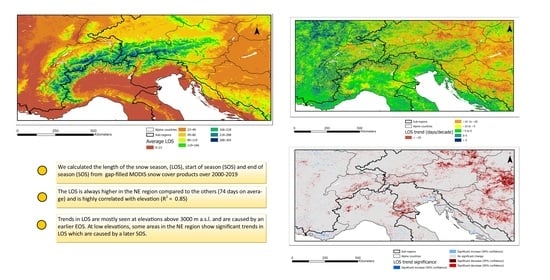
Figure 2.
(a) Average length of the snow cover season expressed in days (LOS); (b) start of the snow cover season expressed in days from the 1st of October (SOS) and (c) end of the snow cover season expressed in days from the 1st of October (EOS) in the GAR during 2000–2019.
Figure 2.
(a) Average length of the snow cover season expressed in days (LOS); (b) start of the snow cover season expressed in days from the 1st of October (SOS) and (c) end of the snow cover season expressed in days from the 1st of October (EOS) in the GAR during 2000–2019.

Figure 3.
Quantiles of the distribution of LOS average values in the 2000–2019 period in each 5-m interval of the GAR elevation range.
Figure 3.
Quantiles of the distribution of LOS average values in the 2000–2019 period in each 5-m interval of the GAR elevation range.

Figure 4.
Differences between the LOS grid point values and the medians of the distributions of the GAR LOS values falling in the corresponding 5-m elevation intervals.
Figure 4.
Differences between the LOS grid point values and the medians of the distributions of the GAR LOS values falling in the corresponding 5-m elevation intervals.

Figure 5.
(a) Standard deviations of the snow cover season length (LOS) in the 2000–2019 period expressed in days; (b) ratio between the LOS standard deviations and LOS mean values; (c) quantiles of the distribution of the ratios between the LOS standard deviations and LOS mean values in each 5-m interval of the GAR elevation range.

Figure 6.
Average Length of Season (LOS) during 2000–2019 in the Greater Alpine Region (GAR) and four subregions.
Figure 6.
Average Length of Season (LOS) during 2000–2019 in the Greater Alpine Region (GAR) and four subregions.

Figure 7.
Average Length of Season (LOS) during 2000–2019 in the four subregions of the Greater Alpine Region by elevation band.
Figure 7.
Average Length of Season (LOS) during 2000–2019 in the four subregions of the Greater Alpine Region by elevation band.

Figure 8.
Frequency of negative and positive significant trends (95% confidence level) in the length of season (LOS) normalized by the number of grid cells in each elevation band in the Greater Alpine Region.
Figure 8.
Frequency of negative and positive significant trends (95% confidence level) in the length of season (LOS) normalized by the number of grid cells in each elevation band in the Greater Alpine Region.

Figure 9.
(a): trend in the length of season (LOS) in days per decade in the Greater Alpine region from 2000 to 2019. (b): significance of the trends in the LOS over the GAR.
Figure 9.
(a): trend in the length of season (LOS) in days per decade in the Greater Alpine region from 2000 to 2019. (b): significance of the trends in the LOS over the GAR.

Figure 10.
(a) Frequency of the significant trends (95% confidence level) in the length of season (LOS) normalized by the number of grid cells in each elevation band in the Greater Alpine Region by filtering out grid cells with varying glacier coverage from the Randolph glacier inventory). (b): Frequency of the significant trends (95% confidence level) in the length of season (LOS) normalized by the number of grid cells in each elevation band in the Greater Alpine Region when all glacier cells are removed. (c,d) show examples of glacier groups (Aletsch, Switzerland and Mont Blanc, Italy/France) with the trends superimposed.


Table 1.
Correspondence between the day of the hydrological year and calendar date for the grid points with continuous snow cover.
Table 1.
Correspondence between the day of the hydrological year and calendar date for the grid points with continuous snow cover.
| Date | Corresponding Day |
|---|---|
| 1 October | 1 |
| 16 October | 16 |
| 31 October | 31 |
| 15 November | 46 |
| 30 November | 61 |
| 15 December | 76 |
| 30 December | 91 |
| 14 January | 106 |
| 29 January | 121 |
| 13 February | 136 |
| 28 February | 151 |
| 15 March | 166 |
| 30 March | 181 |
| 14 April | 196 |
| 29 April | 211 |
| 14 May | 226 |
| 29 May | 241 |
| 13 June | 256 |
| 28 June | 271 |
| 13 July | 286 |
| 28 July | 301 |
| 12 August | 316 |
| 27 August | 331 |
| 11 September | 346 |
| 26 September | 361 |
Table 2.
Variance explained by multilinear regression and linear regression of individual variables against the three metrics in the GAR. Each cell reports the R2.
Table 2.
Variance explained by multilinear regression and linear regression of individual variables against the three metrics in the GAR. Each cell reports the R2.
| Metric | Multilinear Regression | Elevation | Aspect | Slope | Shading Index | Latitude | Longitude |
|---|---|---|---|---|---|---|---|
| LOS | 0.91 | 0.85 | 0.00 | 0.36 | 0.22 | 0.02 | 0.00 |
| SOS | 0.89 | 0.76 | 0.01 | 0.34 | 0.23 | 0.06 | 0.00 |
| EOS | 0.89 | 0.86 | 0.00 | 0.36 | 0.20 | 0.01 | 0.00 |
Table 3.
Variance explained by the linear regression of individual variables against the three metrics in the GAR for different elevation classes. Elevation is removed by subtracting the average in each 5-m elevation interval, and a linear regression is applied to the residuals. z represents elevation (m a.s.l.). Each cell reports the R2.
| Length of Season | ||||||
|---|---|---|---|---|---|---|
| Elevation Class | Multivariate Regression | Aspect | Slope | Shading | Latitude | Longitude |
| z < 1000 | 0.55 | 0.02 | 0.03 | 0.00 | 0.30 | 0.21 |
| 1000 < z < 2000 | 0.55 | 0.11 | 0.00 | 0.07 | 0.34 | 0.07 |
| 2000 < z < 3000 | 0.34 | 0.12 | 0.00 | 0.07 | 0.20 | 0.06 |
| 3000 < z < 4000 | 0.22 | 0.03 | 0.00 | 0.02 | 0.17 | 0.07 |
| z > 4000 | 0.14 | 0.05 | 0.00 | 0.04 | 0.06 | 0.00 |
| Start of Season | ||||||
| Elevation Class | Multivariate Regression | Aspect | Slope | Shading | Latitude | Longitude |
| z < 1000 | 0.55 | 0.02 | 0.02 | 0.01 | 0.34 | 0.17 |
| 1000 < z < 2000 | 0.57 | 0.12 | 0.00 | 0.08 | 0.33 | 0.08 |
| 2000 < z < 3000 | 0.48 | 0.18 | 0.00 | 0.13 | 0.29 | 0.13 |
| 3000 < z < 4000 | 0.27 | 0.05 | 0.00 | 0.02 | 0.22 | 0.12 |
| z > 4000 | 0.13 | 0.06 | 0.00 | 0.03 | 0.04 | 0.00 |
| End of Season | ||||||
| Elevation Class | Multivariate Regression | Aspect | Slope | Shading | Latitude | Longitude |
| z < 1000 | 0.52 | 0.01 | 0.03 | 0.00 | 0.22 | 0.25 |
| 1000 < z < 2000 | 0.47 | 0.09 | 0.00 | 0.05 | 0.30 | 0.05 |
| 2000 < z < 3000 | 0.28 | 0.10 | 0.00 | 0.04 | 0.16 | 0.04 |
| 3000 < z < 4000 | 0.21 | 0.03 | 0.00 | 0.02 | 0.16 | 0.06 |
| z > 4000 | 0.14 | 0.04 | 0.01 | 0.04 | 0.06 | 0.00 |
Table 4.
Variance explained by the linear regression of individual variables against the three metrics in the GAR for different LOS (length of season) classes. Elevation is removed by subtracting the average in each 5-m elevation interval, and a linear regression is applied to the residuals. Each cell reports the R2.
| Length of Season | ||||||
|---|---|---|---|---|---|---|
| LOS Class | Multivariate Regression | Aspect | Slope | Shading | Latitude | Longitude |
| LOS < 180 | 0.52 | 0.03 | 0.03 | 0.00 | 0.28 | 0.17 |
| 180 < LOS < 330 | 0.40 | 0.12 | 0.00 | 0.09 | 0.28 | 0.14 |
| LOS > 330 | 0.32 | 0.04 | 0.00 | 0.14 | 0.12 | 0.03 |
| Start of Season | ||||||
| LOS Class | Multivariate Regression | Aspect | Slope | Shading | Latitude | Longitude |
| LOS < 180 | 0.53 | 0.03 | 0.02 | 0.00 | 0.32 | 0.15 |
| 180 < LOS < 330 | 0.53 | 0.16 | 0.01 | 0.15 | 0.35 | 0.18 |
| LOS > 330 | 0.32 | 0.05 | 0.00 | 0.15 | 0.13 | 0.04 |
| End of Season | ||||||
| LOS Class | Multivariate Regression | Aspect | Slope | Shading | Latitude | Longitude |
| LOS < 180 | 0.45 | 0.02 | 0.05 | 0.00 | 0.20 | 0.17 |
| 180 < LOS < 330 | 0.31 | 0.09 | 0.00 | 0.06 | 0.23 | 0.11 |
| LOS > 330 | 0.31 | 0.04 | 0.00 | 0.14 | 0.12 | 0.03 |
Table 5.
Trends in the snow cover metrics by elevation band and subregion in days per decade. * Indicates a trend significant at the 90% confidence level; ** indicates a trend significant at the 95% confidence level.
Table 5.
Trends in the snow cover metrics by elevation band and subregion in days per decade. * Indicates a trend significant at the 90% confidence level; ** indicates a trend significant at the 95% confidence level.
| Length of Season | |||||
|---|---|---|---|---|---|
| NW Trend | NE Trend | SW Trend | SE Trend | GAR Trend | |
| 0–500 | − | − | − | − | − |
| 500–1000 | − | − | − | − | − |
| 1000–1500 | + | − | − | − | − |
| 1500–2000 | − | − | − | − | − |
| 2000–2500 | + | − | + | − | − |
| 2500–3000 | − | − | + | − | − |
| 3000–3500 | −6.3 ** | −5.4 ** | − | − | −5.2 * |
| 3500–4000 | −1.1 * | − | −1.6 * | − | −1.2 ** |
| 4000–4500 | − | N/A | − | N/A | − |
| >4500 | + | N/A | + | N/A | + |
| Start of Season | |||||
| NW Trend | NE Trend | SW Trend | SE Trend | GAR Trend | |
| 0–500 | − | + | + | + | + |
| 500–1000 | + | + | + | + | + |
| 1000–1500 | − | + | + | + | + |
| 1500–2000 | + | + | + | + | + |
| 2000–2500 | + | + | + | + | + |
| 2500–3000 | + | + | + | + | + |
| 3000–3500 | 1.6 * | 0.6 ** | + | 0.1 * | + |
| 3500–4000 | 0.1 ** | + | + | 0.1 * | + |
| 4000–4500 | + | N/A | + | N/A | 0.1 |
| >4500 | + | N/A | + | N/A | + |
| End of Season | |||||
| NW Trend | NE Trend | SW Trend | SE Trend | GAR Trend | |
| 0–500 | + | - | + | - | - |
| 500–1000 | + | + | + | + | − |
| 1000–1500 | + | + | + | + | + |
| 1500–2000 | + | − | + | + | + |
| 2000–2500 | − | − | + | + | − |
| 2500–3000 | − | − | + | − | − |
| 3000–3500 | − | − | − | − | − |
| 3500–4000 | − | − | − | − | − |
| 4000–4500 | − | N/A | − | N/A | − |
| >4500 | + | N/A | + | N/A | + |
Table 6.
Trends in the snow cover metrics for different subregions and elevation bands in days per decade. Glacier cells are omitted. * Indicates trends significant at the 90% confidence level; ** indicates trends significant at the 95% confidence level. Only the elevation bands between 2500 and 4500 m a.s.l. are shown.
| NW Trend | NE Trend | SW Trend | SE Trend | GAR Trend | |
|---|---|---|---|---|---|
| Length of Season | |||||
| 2500–3000 | − | − | + | − | − |
| 3000–3500 | − | −11.7 ** | − | − | − |
| 3500–4000 | −4.9 ** | N/A | −7.7 ** | N/A | −6.3 ** |
| 4000–4500 | + | N/A | −5.6 ** | N/A | −2.7 ** |
| Start of Season | |||||
| 2500–3000 | + | + | + | + | + |
| 3000–3500 | + | +2.5 ** | + | + | + |
| 3500–4000 | 0.6 ** | N/A | + | N/A | + |
| 4000–4500 | + | N/A | 1.1 * | N/A | 0.5 * |
| End of Season | |||||
| 2500–3000 | − | − | + | − | − |
| 3000–3500 | − | − | − | − | − |
| 3500–4000 | −4.1 ** | N/A | −5.5 * | N/A | −5.2 * |
| 4000–4500 | + | N/A | −5.0 ** | N/A | −2.5 ** |
Publisher’s Note: MDPI stays neutral with regard to jurisdictional claims in published maps and institutional affiliations. |
© 2021 by the authors. Licensee MDPI, Basel, Switzerland. This article is an open access article distributed under the terms and conditions of the Creative Commons Attribution (CC BY) license (https://creativecommons.org/licenses/by/4.0/).
Share and Cite
MDPI and ACS Style
Fugazza, D.; Manara, V.; Senese, A.; Diolaiuti, G.; Maugeri, M. Snow Cover Variability in the Greater Alpine Region in the MODIS Era (2000–2019). Remote Sens. 2021, 13, 2945. https://doi.org/10.3390/rs13152945
AMA Style
Fugazza D, Manara V, Senese A, Diolaiuti G, Maugeri M. Snow Cover Variability in the Greater Alpine Region in the MODIS Era (2000–2019). Remote Sensing. 2021; 13(15):2945. https://doi.org/10.3390/rs13152945
Chicago/Turabian StyleFugazza, Davide, Veronica Manara, Antonella Senese, Guglielmina Diolaiuti, and Maurizio Maugeri. 2021. "Snow Cover Variability in the Greater Alpine Region in the MODIS Era (2000–2019)" Remote Sensing 13, no. 15: 2945. https://doi.org/10.3390/rs13152945
Note that from the first issue of 2016, this journal uses article numbers instead of page numbers. See further details here.