
A Deep Learning Approach to an Enhanced Building Footprint and Road Detection in High-Resolution Satellite Imagery


1
Tracasa Instrumental, Calle Cabárceno 6, 31621 Sarriguren, Spain
2
Institute of Smart Cities (ISC), Public University of Navarre (UPNA), Arrosadia Campus, 31006 Pamplona, Spain
*
Author to whom correspondence should be addressed.
Remote Sens. 2021, 13(16), 3135; https://doi.org/10.3390/rs13163135
Submission received: 16 July 2021
/
Revised: 3 August 2021
/
Accepted: 4 August 2021
/
Published: 7 August 2021
(This article belongs to the Special Issue Computer Vision and Deep Learning for Remote Sensing Applications)
Abstract
:The detection of building footprints and road networks has many useful applications including the monitoring of urban development, real-time navigation, etc. Taking into account that a great deal of human attention is required by these remote sensing tasks, a lot of effort has been made to automate them. However, the vast majority of the approaches rely on very high-resolution satellite imagery (<2.5 m) whose costs are not yet affordable for maintaining up-to-date maps. Working with the limited spatial resolution provided by high-resolution satellite imagery such as Sentinel-1 and Sentinel-2 (10 m) makes it hard to detect buildings and roads, since these labels may coexist within the same pixel. This paper focuses on this problem and presents a novel methodology capable of detecting building and roads with sub-pixel width by increasing the resolution of the output masks. This methodology consists of fusing Sentinel-1 and Sentinel-2 data (at 10 m) together with OpenStreetMap to train deep learning models for building and road detection at 2.5 m. This becomes possible thanks to the usage of OpenStreetMap vector data, which can be rasterized to any desired resolution. Accordingly, a few simple yet effective modifications of the U-Net architecture are proposed to not only semantically segment the input image, but also to learn how to enhance the resolution of the output masks. As a result, generated mappings quadruplicate the input spatial resolution, closing the gap between satellite and aerial imagery for building and road detection. To properly evaluate the generalization capabilities of the proposed methodology, a data-set composed of 44 cities across the Spanish territory have been considered and divided into training and testing cities. Both quantitative and qualitative results show that high-resolution satellite imagery can be used for sub-pixel width building and road detection following the proper methodology.
1. Introduction
Nowadays the detection of building footprints and the extraction of road networks have become one the most important remote sensing tasks, since they are of paramount importance for countries to better understand the impacts of urban growing in different ecosystems. To date, these tasks have been mainly performed by human experts, occasionally assisted by semi-automatic tools, resulting in a very costly and time-consuming process. Therefore, in the last few years, there have been a great deal of automation approaches that combine satellite imagery with machine learning models [1,2,3]. However, the scarcity of open high-resolution earth observation data is one of the main challenges for developing models that automatically generate fine-grained up-to-date building and road mappings.
Currently, Earth Observation (EO) data is becoming more accessible and affordable thanks to the Copernicus programme [4] coordinated and managed by the European Commission in partnership with the European Space Agency (ESA). The ESA is developing seven Sentinel missions under the Copernicus Programme focusing on providing data for monitoring different Earth aspects such as the atmosphere, oceans, or lands. The Copernicus Programme is alleviating the lack of high-resolution EO data making the information produced in the framework of Copernicus available free-of-charge to all its users and the public. However, an accurate detection of buildings and roads remains a challenge due to the limited spatial resolution offered.
Among the Sentinel missions, Sentinel-1 (S1) and Sentinel-2 (S2) are the most well-suited for the extraction of building footprints and road networks. S2 is a multi-spectral sensor mainly dedicated to the control of emerged lands and coastal profiles on a global scale [5]. S2 provides high-resolution optical images composed of thirteen bands, principally in the visible/near infrared (VNIR) and short-wave infrared spectral range (SWIR) with resolutions ranging from 10 m to 60 m. S1, on the other hand, provides Ground Range Detected (GRD) data from a dual-polarization C-band Synthetic Aperture Radar (SAR) instrument [6] at different spatial resolutions (down to 5 m). SAR instruments can acquire meaningful data during daytime and nighttime regardless of weather conditions.
The fusion of optical and SAR data is an active area of research and it has proven successful for different remote sensing tasks [7,8]. In this regard, S1 and S2 complement each other perfectly due to their different characteristics, facilitating the mapping tasks [9], although few works have considered using them together for pixel-wise labeling purposes [10,11]. In fact, to the best of our knowledge, there is no prior work combining S1 and S2 for building and road detection.
Both building footprint detection and road network extraction tasks can be formulated as pixel labeling problems. Accurate pixel-wise labeling of a large satellite image is a complex task for a human given the vast diversity of terrestrial objects. Not only the variations in their shapes, but also occlusions and shadows may increase the difficulty of this task [12]. Furthermore, the spatial resolution of the imagery taken as input plays an important role. The greater the spatial resolution is, the easier it will be not only for experts but also for machine learning models to cope with complex scenarios, enhancing the labeling process. For this reason, S1 and S2 images are not usually considered for fine-grained building and road mappings.
In recent years, deep learning has received a lot of attention in both scientific research and practical application [13,14]. Pixel labeling tasks, also known as semantic segmentation tasks, have benefited from deep learning advancements, clearly outperforming established approaches for applications such as medical image segmentation [15] and autonomous driving semantic segmentation [16]. Deep learning techniques have also been successfully applied to remote sensing tasks [2,3], including the detection of building footprints [12,17] and road networks [18,19]. Nevertheless, the vast majority of works rely on aerial imagery or very high-resolution satellite products for this purpose. To the best of our knowledge, no prior works have attempted to generate building and road segmentation mappings with a greater spatial resolution than the one given at the input.
In order to train robust deep learning models a great deal of labeled data is required. However, the scarcity of accurately labeled data tends to be a limiting factor. Despite the existence of open EO data-sets [20,21], a small portion of them use S1 and S2 imagery. Moreover, their labels tend to be coarse which makes them useless to detect complex elements such as buildings or roads. Furthermore, the spatial resolution of the imagery taken as input is crucial to define the scope of the labeling process. That is, very high-resolution imagery (less than 2.5 m) is usually used to detect fine-grained objects such as building footprints [22], extract road networks [18], and so on, whereas high-resolution imagery (2.5 m to 10 m) is usually limited to wider elements like forests [23], water bodies [24], etc. Contrary to the previous works, we will show that with the proposed methodology, high-resolution imagery (S1 and S2) can also be used to detect complex elements such as buildings or roads accurately. In fact, we will show that we are able to infer 2.5 m semantic segmentation maps from 10 m resolution images, bridging the gap between satellite and aerial imagery for pixel-wise labeling labors.
Hence, our aim is to use S1 and S2 data to produce high-resolution building footprint and road network segmentation maps, showing that open data from Copernicus can allow automating mapping tasks for these classes. To do so, a methodology for generating a deep learning data-set from scratch is presented. To obtain the ground-truth data, OpenStreetMap (OSM) [25] has been used for labeling S1 and S2 imagery giving special attention to the errors inherent to open data such as limited coverage or irregular registrations, which have been tackled with a new concept named as validation masks. These masks filter the samples used to train the models in an efficient way. It is worth noting that the proposed methodology could be extrapolated to any OSM label that can be observed from Sentinel-2 imagery.
In summary, the main novelties of our approach are:
- S2 data (multi-spectral) is fused with S1 data (SAR) making the most of both sensors for building and road detection at a higher resolution (2.5 m) than the input one (10 m).
- A methodology to generate detailed remote sensing data-sets for building footprints and road networks detection using OSM has been developed. Validation masks are proposed for dealing with labeling errors.
- Taking advantage of the high revisit times of the Sentinel missions, a low-cost data augmentation technique is proposed.
- The standard U-Net [15] architecture has been slightly modified given rise to fine-grained segmentation masks. Accordingly, resulting mappings quadruple the input’s spatial resolution.
Overall, we propose an accurate, yet simple and easily reproducible methodology for extracting high quality building and road masks from satellite imagery. To the best of our knowledge, we achieve the greatest accuracy for these tasks using 10 m satellite imagery. To test the proposed methodology, 44 cities across the Spanish territory have been selected and divided into training and testing cities according to machine learning principles [26]. In order to evaluate the performance of the developed models, the mean Intersection over Union metric (mIoU) and the F-score have been used. Experiments demonstrate that using high-resolution satellite imagery is possible to accurately detect complex elements such as building or roads, showing the possibility of quadrupling the resolution at the output up to 2.5 m. Moreover, the increase in the model’s performance when combining optical and SAR data is reassured. Finally, the usefulness of the proposed validation masks to deal with labeling errors inherent to open databases such as OSM is proved.
The remainder of this article is organized as follows. Deep learning and convolutional neural networks (CNNs), focusing on building and road detection, are briefly recalled in Section 2. Thereafter, our proposal for automated building footprint and road network extraction fusing S1, S2, and OSM data is detailed in Section 3. Then, the experimental framework, experiments and results are presented and discussed in Section 5. Finally, Section 6 concludes this work and present some future research.
2. Related Works
This section is divided into four subsections. Firstly, deep learning and the application of CNNs to remote sensing tasks are outlined in Section 2.1. Thereafter, the usage of deep learning in satellite imagery segmentation is described in Section 2.2, paying special attention to the use of S1 and S2 sensors. Then, in Section 2.3 recent approaches for building footprint detection and road network extraction are briefly recalled. Finally, the capabilities of open databases for remote sensing data-set labeling are assessed in Section 2.4.
2.1. Deep Learning, Convolutional Neural Networks, and Semantic Segmentation
Deep learning has been one of the major breakthroughs in artificial intelligence during the last decade, showing many successful applications. With respect to computer vision and image processing, CNNs have become the standard for almost every task such as image classification [27], object detection [28], or semantic segmentation [16]. For this reason, we have focused on CNN-based semantic segmentation.
The first network for semantic segmentation tasks was proposed by Long et al. [29] and named as Fully Convolutional Network (FCN). It was one of the first CNN-based semantic segmentation methods where the segmentation map was obtained through a single forward pass. Shortly thereafter, U-Net [15] was proposed, based on FCN, where the encoder-decoder structure enhanced the segmentation quality. U-Net can be seen as a convolutional auto-encoder [30] that predicts pixel-wise class labels instead of predicting the input image again. In this architecture, feature maps are shared between the encoder and decoder to propagate context information to higher resolution layers. Despite the simplicity of its structure, U-Net produces precise segmentation maps and hence, it has been employed in many studies to get better performance in various fields [31,32], including remote sensing [2,3].
2.2. Deep Learning in Remote Sensing: Applications Using Sentinel-1 and Sentinel-2
The geoscience community has rapidly adopted deep learning-based methods for many applications [2], including remote sensing tasks [3,33]. The accuracy level that can be obtained across different remote sensing tasks highly depends on the characteristics of the sensors, especially on their spatial resolution [34]. In this regard, sensors which provide lower resolution products are mainly used for image recognition of whole image chips [35], so-called scene labeling, whereas, sensors with a higher resolution are used for a wider range of tasks including image segmentation [36] and object detection [37].
S2 has established itself as the leading high-resolution multi-spectral sensor for remote sensing tasks, partly, due to the free availability of its products. However, due to its limited spatial resolution, its products have been mostly used for scene labeling tasks [35]. Accordingly, many data-sets have been recently released aiming at pushing remote sensing research with S2 [20,21].
In the last years, growing attention has been given to S1 focusing on flood mappings [38] and land cover classification of agricultural areas [39]. However, little research has been conducted to assess the S1’s GRD data capabilities for detecting more complex elements such as buildings or roads. Taking into account the characteristics of S2 and S1, both sensors complements each other perfectly. A great deal of data-sets have also been recently released aiming at making the most of this synergy [10,11]. However, they do not deal with specific labels such as roads or buildings.
In spite of the upward trend in the number of released S1 and S2 remote sensing data-sets, the volume of annotated images is relatively small. Moreover, the vast majority of public data-sets are focused on scene labeling tasks [20,35]. The few of them that are oriented to semantic segmentation tasks [11,21] have coarse labels limiting their application for problems where a high degree of detail is required. Thus, they are insufficient to train robust CNN-based high-resolution semantic segmentation models. One way of tackling this problem is using open databases for labeling purposes. We recall works related to this procedure in Section 2.4.
2.3. Semantic Segmentation of Buildings and Roads
Promising building footprint detection approaches have been proposed in the literature. Wagner et al. [40] presented a modified U-Net capable of discriminating between adjacent buildings. To incorporate the structure information of buildings, Hui et al. [41] opted for a multi-task learning strategy, replacing the vanilla U-Net encoder with an Xception module. A similar approach was taken by Guo et al. [42], incorporating lightweight soft-attention mechanisms to deal with the large intraclass variance of buildings.
Regarding the road network extraction task, several approaches have been developed in recent years. Zhang et al. [43] combined the strengths of residual learning with the U-Net architecture aiming at facilitating the propagation of information while reducing the number of parameters. On the other hand, Zhou et al. [44] opted for a LinkNet architecture with a pre-trained encoder and dilated Convolutions (D-LinkNet) to enlarge the receptive field without diminishing the resolution of the feature maps. The D-LinkNet architecture was recently rebuilt by Fan et al. [45], replacing the ResNet backbone with a ResNeXt.
However, these works make use of aerial imagery (<1 m) to produce detailed building and road mappings. Consequently, the high costs of those products limits the possibility of keeping building and road maps up-to-date. Despite not being, a priori, the most adequate sensor for detecting complex elements such as buildings and roads due to its limited spatial resolution [34,46], a few works have focused on assessing the capabilities of S1 and S2 imagery for the extraction of buildings and roads.
Helber et al. [31] and Rapuzzi et al. [47] aimed at detecting building footprints using different versions of the U-Net architecture. Whereas the former relied on S2 imagery, the latter opted for using S1 data. A similar approach was taken by Oehmcke et al. [48] to detect hardly visible roads using S2 time series. On the other hand, Abdelfattah et al. [49] proposed a semi-automatic approach to extract off-roads and trails from S1 imagery.
Nevertheless, the aforementioned works resulted in coarse building and road mappings, drastically hindering their application. Nonetheless, our hypothesis is that minor tweaks in the architecture and an appropriate methodology may lead to huge improvements on the detection tasks. In fact, our hypothesis is that the output resolution can achieve sub-pixel width accuracy, that is, segmentation maps at higher resolution than the original one (10 m). To the best of our knowledge, no previous attempts have been made in this direction.
2.4. Open Data for Deep Learning Labeling
When freely-available remote sensing data-sets do not meet the requirements, databases such as OSM may come in handy [50]. Accordingly, vector data from OSM is rasterized (transformed to pixel coordinates) to generate the ground truth masks for training. However, there are two types of labeling noise present in OSM that could have a negative impact on the learning of deep learning models:
- Omission noise: refers to an object, clearly visible in a satellite/aerial image, which has not been labeled. This type of noise is particularly noticeable in the building labels, since many rural-areas are not completely labeled in OSM. Moreover, small roads and alleys also suffer from omission noise, commonly being omitted from maps.
- Registration noise: refers to an object which has been labeled but its location in the map is inaccurate. Due to the greater spatial resolution, labeling misalignment are more noticeable when dealing with aerial imagery.
Mnih et al. [19] proposed to reduce both omission and registration errors at training time using two robust loss functions. Li et al. [51], on the other hand, undertook the misalignment between OSM building footprints and satellite imagery caused by different projections and accuracy levels from data sources, when generating the data-set. Others such as Kaiser et al. [50] proposed to perform a large-scale pre-training using the full data-set and then, apply a domain adaptation with hand-labeled data. As it will be explained in Section 3.2, we will take this approach but highly reducing data-set hand-labeling costs through the use of the proposed validation masks.
3. Proposal: Enhanced Building Footprint and Road Network Detection
The proposal consists in a simple and reproducible methodology to use S1 and S2 data together with OSM to generate deep learning models for sub-pixel width building footprint and road network detection. We will not only show the capabilities of S1 and S2 data fusion, but also make use of them to output a higher resolution mapping than the input resolution. That is, whereas the maximum resolution used for S1 and S2 will be 10 m, the output mappings will be at 2.5 m resolution. Although this work is focused on extracting building and roads, the proposed methodology could be extrapolated to any desired OSM label that can be observed from S2 imagery.
Figure 1 gives an overview of our approach, whose modules will be further described in the following sections. We explain how to generate the data-set in Section 3.1 (Module A). Section 3.2 (Module B) delves into the validation masks generation process. Finally, modifications proposed for the U-Net network are presented in Section 3.3 (Module C).
3.1. Data-Set Generation
Pixel labeling tasks are the most common remote sensing tasks. Training deep learning-based models requires image pairs representing the scene and the desired labeling. In this work, we fused five S2 bands with two S1 bands to build our inputs, whereas OSM has been used to generate the target labeling (although any other data source could be used either for the inputs or the outputs). Briefly, the goal is to produce a complete semantic segmentation of a satellite image. In this scenario, the availability of accurately labeled data for training tends to be the limiting factor when automating tasks using deep learning-based approaches. Despite the fact that hand-labeled data tends to be reasonably accurate, the cost of manual labeling and the lack of publicly available hand-labeled data-sets strongly restricts the size of the training and testing sets for remote sensing tasks.
Crowd-sourced projects such as OSM may come in handy when generating remote sensing data-sets. Portals such as Geofabrik [52] exploit OSM data in order to freely provide ready-to-use geodata to the public. Accordingly, it is now possible to construct data-sets that are much larger than the ones that have been hand-labeled. The use of these larger data-sets has improved the performance of deep learning methods on some remote sensing tasks [22,53].
The data-set used in this paper has been generated following the workflow shown in Module A on Figure 1. The processing steps for a generic area of interest are described hereafter. Notice that the final training set will be formed using several areas.
Firstly, S2 products are queried and downloaded from the Sentinels Scientific Data Hub (SciHub) [54], given a bounding box, a time interval, and a maximum cloud cover percentage of 5. Depending on the extent of the bounding box, multiple S2 products may be required. Therefore, products are filtered ensuring a full bounding box coverage and, at the same time, minimizing the temporal distance between them as well as the overall cloud cover percentage and maximizing their solar zenith angle at acquisition time [55].
Even though S2 offers thirteen multi-spectral bands, we only made use of the Red, Green, Blue, and Near Infrared bands as they are the only ones provided at the greatest resolution of 10 m. Additionally, the Normalized Difference Vegetation Index (NDVI) is computed considering it is a reliable source of information about impervious surfaces in urban spaces [56]. Obviously, there will be exceptions such as buildings whose roofs are covered by grass. In these cases, the CNNs should be capable of understanding the geometries and the surroundings to properly label the buildings.
Regarding S1, we have worked with the Level-1 GRD product in Interferometric Wide (IW) swath mode. That product combines a swath width of 250 km with a moderate resolution of m (depending on the beam id) and could be provided in four polarization modes (VV, VH, HH, HV). However, our approach only considers dual vertical polarization (VV, VH), since dual horizontal polarization (HH, HV) is limited to polar regions. S1 products were firstly downloaded from the SciHub filtering using as time interval 7 days ± the mean of the ingestion times of the S2 products considered in the previous step. Then different pre-processing steps were applied. Firstly, backscatter intensities were calculated using the GRD metadata in the radiometric calibration step. Thereafter, the side looking effects were corrected using the Digital Elevation Model (DEM) from the Shuttle Radar Topography Mission (SRTM) in the terrain correction step. Finally, backscatter intensities were log-scaled from Chi-squared to Gaussian distribution and converted to decibels. Note that S1 pre-processing workflow follows the recommendations in [57] and has been made within the Sentinel application platform (SNAP) [58], a common architecture for all Sentinel satellite toolboxes.
Resulting bands from S1 and S2 are then stacked to create the 7-band inputs. Regarding ground-truth data, OSM is used to generate the masks. Due to the plethora of OSM classes available, we perform a reclassification, aggregating different classes on the basis of the desired legend. Hence, a great deal of road types (OSM codes 5111-5115, 5121-5124, and 5132-5134) constitute the label road, whereas building polygon outlines (OSM code 1500) comprise the label building. It should be noted that as OSM contains vector data that must be rasterized. According to the low spatial resolution of the imagery used (10 m), buildings are filtered, discarding those whose surface area is inferior to 50 m. Likewise, since roads came as line-strings, we buffered them to 10 m before rasterizing. Taking into account that roads are not always 10 m width, we firstly rasterize roads and then buildings into the same mask to make them more realistic. It is worth stressing that ground-truth masks are generated at both 10 m and 2.5 m to evaluate the x1 and x4 models, respectively.
Additionally, for the same generic area, we propose a data augmentation technique based on using several images from the same place at different time-steps. This is possible thanks to the high revisit times of S1 and S2. In this way, a temporal component is added to the data-set. As we will show in the experimental framework in Section 4.1, in this paper we consider data from the four seasons of a year, but this could be arbitrarily increased up to 70 time-steps on the equator per year. It must be noted that many studies have already used multi-temporal Sentinel images for a wide range of use cases such as crop type classification [59] or tree species classification [60]. However, our approach differs from the standard way of dealing with image time series in deep learning, which mainly consist on combining CNNs with Recurrent Neural Networks. In this work, the temporal information will only be used to increase the diversity of the samples used to feed the models. That is, a color data augmentation is applied but using real Sentinel images from different timestamps. Note that we will also test the proposal in different time frames.
3.2. Validation Masks
Despite that the data-set may seem ready to be used to train deep learning-based models, if we carefully analyze the data-set we will notice that a great deal of labeling noise is present due to the usage of OSM. Additionally, we will also find sensing noise which cannot be easily overcome trough pre-processing techniques (e.g., artifacts due to planes crossing the sensing area). Since high-quality data is crucial in order to develop robust models, we propose the use of validation masks at both training and testing times. Validation masks are the result of splitting an image into multiple tiles and labeling each tile as valid or not valid, depending on the quality of its corresponding ground-truth mask. The use of validations masks at training time is optional since it is possible to achieve a high performance without them. However, they are of great importance to achieve the maximum level of accuracy as we will show in Section 5.3. In particular, we propose performing a large-scale pre-training using all the available OSM data (without further treatment) and then, fine-tune for a few epochs making use of the validation masks. It must be noted that validation masks are always used when testing the models to carry out a fair evaluation.
As explained in Section 2.3, either registration or omission noise can occur when using OSM for automatic labeling. Luckily, when labeling S1 and S2 images, registration errors become unnoticeable due to the limited spatial resolution. Therefore, in this work we focused on omission noise and sensing errors. Accordingly, two types of validation masks are defined:
- Sensor validation masks: contain information related to low quality data resulting from sensing errors such as the presence of clouds, shadows, etc.
- Label-specific validation masks: address omission noise derived from the use of open databases such as OSM. Specific validation masks are individually generated for each target label (building and road), allowing one to reuse those masks when building up different legends.
Both validation masks are manually generated by visual inspection as shown in Module B on Figure 1. It should be highlighted that the spatial resolution of those masks has been reduced to 640 m, aiming at saving time and effort during their generation (for a city such as Barcelona North in Figure 2, just 18 × 27 pixels need to be annotated, which takes approximately 5 min using QGIS [61]). Therefore, validation masks are fast to label, orders of magnitude faster than manual labeling the whole scene, which is the common practice. Moreover, it must be noted that third party applications such as cloud detectors could be easily included to semi-automate some hand-labeling tasks, reducing human intervention. To better understand this concept, sensor and road-specific validation masks are presented in Figure 2 along with the corresponding RGB image and ground truth for Barcelona North city (included in our data-set).
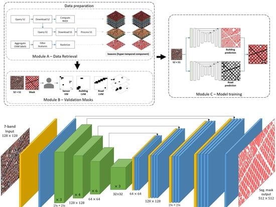
3.3. Network Implementation
Our model is based on Fully Convolutional Networks (FCNs) and U-Net architecture. Figure 3 illustrates the architectures we have used for building footprint and road detection. As shown in Figure 3, the U-Net network consists of a contracting path to capture context and an expansive path to refine localization, which is symmetrical to the former and gives it the u-shaped architecture. The down-sampling or contracting part has a FCN-like architecture that extracts features with convolutions. The up-sampling path uses up-convolutions, increasing the dimensions of the feature maps while reducing their number. Among the main novelties of the U-Net architecture, there is the concatenation of feature maps between the down-sampling and up-sampling parts. Moreover, the sharing of feature maps avoids losing pattern information and hence, enables precise localization. Finally, a convolution processes the feature maps to generate a segmentation map that categorizes each pixel of the input image.
In this work we have replaced the original U-Net encoder with a ResNet-34 [62] on account of the density and precision of the features extracted by residuals models. Moreover, residual connections exploit all the information available along the down-sampling process while reducing the computational cost.
Semantic segmentation of satellite imagery with a spatial resolution of 10 m results in blurry and imprecise segmentation masks. This is due to the coexistence of multiple labels in a single pixel. Recognizing this issue, this paper raises the possibility of enhancing the spatial resolution of the mappings resulting from the segmentation of S1 and S2 imagery at 10 m. In particular, we propose to increase the output resolution up to 2.5 m (4 times larger than the input). This is possible due to the nature of OSM, whose data in vector format can be rasterized to any desired resolution. For this purpose, two strategies have been contemplated:
- Deconvolution (up-sampling at the output): To append two extra deconvolutional layers to the decoder (Figure 3a). Note that, this approach prevents the deconvolutional layers from getting contextual information due to the lack of shared weights (there are no same-level layers on the contraction path). However, the computational cost is lower compared to increasing the resolution at the input.
- Input re-scaling (up-sampling at the input): To increase the input resolution before the feature extractor (Figure 3b). On the one hand, this outlook allows one to keep the network architecture unaltered, avoiding losing pattern information. However, the increase in the input resolution has a negative effect on the computational cost. In order to enhance input’s resolution two classical interpolation algorithms have been considered (Bicubic and Nearest Neighbor) as well as a state-of-the-art S2 super-resolution approach (Galar et al. [63]).
3.4. Network Training
FCNs are usually fed with fixed-size patches, generated by tiling every image in the data-set. However, that may lead to overfitting considering it is quite likely that patches pass through the network more than once. Therefore, we have opted for using random tiles rather than fixed ones. Despite the fact that increasing tile variability making it almost impossible for the model to see a sample twice, other training issues should be addressed. We may find not only samples which are extremely unbalanced due to the randomness, but also samples containing labeling errors. That is the reason why in Section 3.2 we introduced the validation masks. Validation masks are used to compute valid sample origins in an efficient but not exhaustive way, which is of great importance considering the large amount of data to be processed. In this way, random patches will only be generated if all their pixels belong to valid zones.
Similarly to other works [40,64,65], we opted for a well-established loss function known as the Combo Loss [66] (Equation (1)), which combines Binary Cross-Entropy [67] (Equation (2)) and Dice Loss [68] (Equation (3)). Briefly, it leverages the flexibility of Dice loss in controlling the trade-off between false-negatives and false-positives whereas, binary cross-entropy is used for curve smoothing.
Two binary semantic segmentation models will be trained, one for detecting building footprints and the other for road networks, respectively. It is worth stressing that resulting segmentation masks could be merged as it is exemplified in Figure 1 to build up more elaborated legends.
4. Experimental Framework
In this section, the experimental framework is described. Section 4.1 presents the data-set. Then, in Section 4.2 details regarding the training procedure are given. Thereafter, in Section 4.3 the performance measures and evaluation criterion are explained. Finally, Section 4.4 introduces the experiments carried out in Section 5.
4.1. Data-Set
The data-set used in further experiments is composed by a selection of 44 cities spread across the Spanish territory. Moreover, the seasonal component comprises 4 trimesters from June 2018 to March 2019. It must be noted that some periods have been discarded in cities mainly due to the substantial presence of clouds, shadows, and other adverse weather conditions. Details about the data-set are presented in Table 1. For each target zone, its dimensions in pixels of 10 m, as well as the total number of tiles comprising the validation masks (64 × 64 pixels) are displayed. Moreover, for each trimester the number of valid tiles corresponding to each target label is included. Finally, the sub-set correspondence is presented. Additionally, the data-set geographical distribution is shown in Figure 4.
The data-set was split into two sub-sets (training and test) according to the machine learning guidelines suggested in [26]. Consequently, each zone is assigned to a single set to prevent data-leakage and make the evaluation fairer. For this reason, trimesters of the same zone cannot be assigned to different sets.
The training set has been used to learn the parameters of the models, whereas the test set has been used to assess the generalization capability of the different architectures. It is noteworthy to mention that through experimentation we decided not make use of a validation set considering that in this specific scenario it would only have increased the training time without anything in exchange. Therefore, we prefer to renounce to the validation set and use its data for training. The set to which each city has been assigned is shown in Table 1. Again, this split has been done in such a way that both sets have a good representation of the different scenarios.
4.2. Training Details
Since no validation set has been used, we take the last epoch model without applying early stopping or model selection based on validation loss. Data augmentation is essential to prevent overfitting, especially when the data-set is too large to fit into memory. Moreover, in large data sets, the use of reasonable data augmentation methods can still improve the performance of the network [69]. In the field of image semantic segmentation, the scarcity of data is more apparent. We augment our data applying horizontal and vertical flips, as well as 90-degree rotations. Despite the fact that color augmentations are usually utilized in building and road detection, their results are unrealistic. Therefore, we have opted for augmenting our data-set in a realistic manner rather than in a synthetic one, including a hyper-temporal component as described in Section 3.1. Additionally, test-time augmentation (TTA) is also applied. That is, the final prediction is obtained as the aggregation of predictions across transformed versions of a test input. In this paper we combine 90-degree rotations with vertical and horizontal flips, resulting in eight different inputs.
With respect to the specific hyper-parameters for the experiments, we use the Adam optimizer [70] with a learning rate of . The batch size has been set to 14 according to the previous guidelines. That is, the maximum number of samples that fits into memory. All the models have been trained for 1000 epochs. Therefore, to properly assess the impact of validation masks, in the third experiment we pre-train the model for 900 epochs and fine-tune for 100 epochs. The experiments have been run on a server equipped with an Intel Xeon E5-2609 v4 @ 1.70 GHz, 64 GB of RAM and 4x NVIDIA RTX 2080Ti GPUs.
4.3. Performance Measures and Evaluation
The performance of each experiment has been quantitatively evaluated using the F-score and the Intersection over Union (IoU) metrics. Notice that ground truth masks have been generated at both 10 m (x1) and 2.5 m (x4) to evaluate the models depending on their output resolution. The metrics are computed twice, considering and not considering a tolerance buffer. Metrics computed using a tolerance buffer can be seen as a relaxed version and hence, we refer to them as relaxed IoU (rlx. IoU) and relaxed F-Score (rlx. F-Score). Using the tolerance buffer the negative impact of mislabeled edge pixels are diminished, which are hard to detect given the limited spatial resolution of the imagery used [12,71]. However, the metrics with respect to the unaltered ground truth are also provided. The tolerance buffer is computed as the union of the erosion of the ground truth (in green) and two times its dilation (in blue) as it is illustrated in Figure 5. Here, the tolerance buffers for a 10 m (x1) and 2.5 m (x4) resolution ground truths are compared. With the usage of these buffers, pixels inside them are not used for metrics computation.
Additionally, the performance of each experiment has been qualitatively evaluated through the visual inspection of the IoU in form of true positives (TP), true negatives (TN), false positives (FP), and false negatives (FN). This approach yields to a better description of how the models are behaving, clearly identifying their differences.
4.4. Summary of Experiments
The experiments carried out in the next section have been devised in such a way that the capabilities of S1 and S2 data fusion for achieving sub-pixel width accuracy extracting buildings and roads are assessed. For this purpose, we will try to answer the following key questions.
- What is the advantage of combining optical and SAR data for building and road detection?
- Can the output resolution be greater than the input resolution?
- How much can the performance be pushed with sensor and label-specific validation masks?
Section 5 attempts to shed light on these questions through individual experiments.
5. Experimental Study
In this section we try to answer the questions posed in Section 4.4 through three experiments:
- Experiment 1: On the goodness of S1 and S2 data fusion: assesses the suitability of optical (S2) and SAR (S1) data, as well as their fusion for building and road extraction tasks.
- Experiment 2: Enhancing the output resolution: evaluates different approaches for enhancing the output resolution up to 2.5 m.
- Experiment 3: Assessing the impact of validation masks: studies the impact the use of validation masks has on the model performance.
5.1. Experiment 1: On the Goodness of S1 and S2 Data Fusion
Here the capabilities of both satellites in terms of building and road extraction are evaluated. To do so, we have trained U-net models using S1 and S2 data individually and combining the data of both satellites (with output resolution at 10 m).
The results in terms of IoU and F-score (and their relaxed versions) in the test set are presented in Table 2. Metrics are presented for each target label (roads and buildings) together with their average. It must be noted that these metrics are computed taking into account only valid pixels, according to the sensor and label-specific validation masks. The best results achieved for each label (building, road and average) and metric are presented in boldface. Finally, a visual comparison in form of segmentation maps over the different approaches is presented in the first row in Figure 6 and Figure 7 for the building and road labels, respectively. Accordingly, each figure’s row corresponds to a different experiment. The last element of each row is directly compared to the elements of the subsequent row. For example, the last element of the second row (S1 + S2) is compared to all the elements of the third row (Deconv x4, EDSR x4, ) in the second experiment.
These results show that S1 struggles to extract roads on its own (0.2376 IoU). Regarding the building detection, S1 is far from being as good as S2 (0.4704 vs. 0.5389 IoU, respectively). However, when fusing S1 and S2 data (S1 + S2), the network is capable of internally learning how to use S1 data to complement S2 data ( achieving 0.5549 and 0.4415 of IoU for building and road labels, respectively). The benefit of combining S1 and S2 data is reflected not only in the metrics (0.4982 vs. 0.4860 avg. IoU, respectively) but also in the figures, showing an improvement in both tasks compared to using only S2 data. With respect to the relaxed versions of the metrics, we can observe that there are slight differences compared with the standard ones, which indicates that the model is not only mislabeling edge pixels, but also failing to properly define structures globally.
5.2. Experiment 2: Enhancing the Output Resolution
In this experiment different alternatives for enhancing the output resolution up to 2.5 m are tested and compared to the standard segmentation approach (without enhancement). Recall that two ways for increasing the output resolution have been proposed, depending on whether the up-scaling is performed at the input or at the output. For the former, three alternatives are considered (EDSR, bicubic, and nearest), whereas for the latter we have used two deconvolutional layers stacked at the end of the network. The results of this experiment are presented in Table 3 and in the third row of Figure 6 and Figure 7.
These results show an increase in the model performance when increasing the output resolution (from 0.4982 up to 0.6004 avg. IoU in the best alternative, Nearest x4). This is due to the greater number of pixels the model has to define the edges of the objects and the objects themselves. As it is reflected on the metrics, models that perform the up-scale at the input outperforms the one doing so at the output (0.5700, 0.5980, and 0.6004 vs. 0.5617 avg. IoU). According to the figures, adding deconvolutional layers at the output produces a behavior similar to the usage of Conditional Random Fields. Since there is no extra information to super-resolve the output, the model is only able to smooth the final output. Finally, Bicubic x4 and Nearest x4 outperform EDSR achieving higher metrics (0.5980 and 0.6004 vs. 0.5700 avg. IoU, respectively) and more fine-grained segmentation masks according to the figures. Accordingly, it seems that the network prefers to internally learn how to super-resolve the input to best fit the segmentation task rather than starting from an already super-resolved input and generating a segmentation mask from it. Overall, Nearest x4 achieves the best metrics (0.6004 vs. 0.5980 avg. IoU, respectively) although Bicubic x4 performs slightly better in terms of roads (0.5982 vs. 0.5986 IoU, respectively). However, this difference is much lower than the one obtained in terms of buildings (0.5974 vs. 0.6027 IoU, respectively). In this case, it must be noted that there are substantial differences between the standard metrics and their relaxed versions, which means that the model is failing to detect edge pixels accurately, due to the limited spatial resolution.
5.3. Experiment 3: Assessing the Impact of Validation Masks
Previous experiments have followed the traditional approach of using all the data available for training the models. However, as it is recalled in Section 3.2, this data may contain a great deal of labeling noise. To get the most out of the available noisy data, previous works [50] proposed pre-training the models using the full data-set and then performing a domain adaptation using hand-labeled data. In this work the sensor and label-specific validation masks have been introduced aiming at reducing the data-set hand-labeling costs. This experiment assesses the impact the use of validations masks has on the model performance. The results of this experiment are presented in Table 4 and in the fourth row of Figure 6 and Figure 7.
There are significant differences between training for 1000 epochs with validation masks VM 1000ep and without them No VM 1000ep (0.5810 vs. 0.6004 avg. IoU, respectively). This is due to the aggressive filtration, drastically reducing the amount of data. However, when pre-training the models for 900 epochs without validation masks and then fine-tuning (FT) for 100 epochs using them, the results are completely different. Note that, the epoch division has been done in such a way that the total number of iterations was the same. Even though SVM greatly increase the performance on the road label (0.6054 vs. 0.5982 IoU, respectively), metrics decrease for the building one (0.5998 vs. 0.6027 IoU, respectively). This is due to the fact that roads are better registered in OSM than buildings. Therefore, the usage of LVM increases the performance on the building label (0.6054 vs. 0.5998 IoU, respectively). As a result, SVM and LVM can be used jointly to push the performance to its limit for both building and road detection (0.6075 of avg. IoU when combining SVM + LVM vs. 0.6004 when no validation masks are used).
5.4. Discussion
Considering the results obtained in the experiments, the following conclusions are drawn:
- Combining optical (S2) and radar (S1) data aids the network to cope with complex scenarios, reducing the negative effect of color spectrum variations.
- Enhancing the resolution at the output gives the model more room for better defining the edges of the objects. Moreover, when using U-Net based architectures enhancing the resolution at the input, the model can take advantage of skip connections resulting in more accurate segmentation masks.
- Validation masks are a simple yet effective artifact to increase the quality of the data, drastically reducing the hand-labeling costs.
To complement the results shown in this paper and to better understand the level of accuracy that can be achieved with this methodology, predicted mappings obtained for Pamplona 2019/03 have been included as Supplementary Materials
. Moreover, aimed at showing the generalization capability of the model presented in this work, road networks have been extracted for the main cities within the Iberian Peninsula. The complete map is available at our webpage (https://tracasa.es/sin-categoria-en/tracasa-succeeds-in-identifying-roads-and-highways-using-images-from-sentinel-satellites-super-resolved-with-artificial-intelligence/ (accessed on 1 August 2021)). In the near future the map will be updated including a building footprint layer.
6. Conclusions and Future Work
This work proposes a simple and reproducible methodology to accurately extract building footprints and road networks from S1 and S2 satellite imagery. Firstly, we have studied the advantages of fusing optical (S2) and SAR (S1) data for these tasks. Thereafter, a few simple modifications have been proposed to the U-Net architecture to enhance the resolution of the generated segmentation mappings. As it can be seen in the quantitative and qualitative results, the model learns internally how to super-resolve the data in order to produce enhanced segmentation masks, sometimes beyond the limits of S2. Finally, since the performance of deep learning-based models is highly dependent on the amount of training data available and, considering that manually labeling is a very costly and time-consuming process, this work sets of an approach to filter large-scale data-sets efficiently. In this regard, a novel artifact named as validation mask is introduced to tackle not only the noise inherent to open data-bases such as OSM, but also sensing errors.
Apart from the novelties proposed in this paper, there are still a few approaches that should be tackled on this topic aiming at making models more robust. Regarding the data-set, more zones could be included for training and testing. Moreover, greater sample variety could be achieved if other continents were taking into account. Likewise, more non-rural areas could be considered in order to extract disseminated buildings and narrow roads. In this regard, the performance of the models can be evaluated in a global setting, comprising different building and road patterns.
Regarding the architecture, bigger feature extractors such as Efficient-Nets could extract richer features in comparison to the actual ResNet-34. However, it would require a bigger computation infrastructure. Additionally, other architectures that exploit SAR and multi-spectral data in a clever and better way should be further studied. Finally, despite the fact that in this work we have opted for quadrupling the output, in the future we would like to study where the enhancement limit is when using S1 and S2 imagery (x8, x10, …).
Supplementary Materials
The following are available online at https://www.mdpi.com/article/10.3390/rs13163135/s1.
Author Contributions
Data curation, R.S.; Investigation, C.A. (Christian Ayala); Supervision, C.A. (Carlos Aranda) and M.G.; Writing—original draft, C.A. (Christian Ayala); Writing—review & editing, C.A. (Christian Ayala) and M.G. All authors have read and agreed to the published version of the manuscript.
Funding
This research received no external funding.
Acknowledgments
Christian Ayala was partially supported by the Goverment of Navarra under the industrial PhD program 2020 reference 0011-1408-2020-000008. Mikel Galar was partially supported by Tracasa Instrumental S.L. under projects OTRI 2018-901-073, OTRI 2019-901-091, and OTRI 2020-901-050, and by the Spanish MICIN (PID2019-108392GB-I00/AEI/10.13039/501100011033).
Conflicts of Interest
The authors declare no conflict of interest.
Abbreviations
| CNN | Convolutional Neural Network |
| DEM | Digital Elevation Model |
| EO | Earth Observation |
| ESA | European Space Agency |
| FCN | Fully Convolutional Network |
| FN | False Negative |
| FP | False Positive |
| GRD | Ground Range Detected |
| IoU | Intersection over Union |
| IW | Interferometric Wide |
| LVM | Label-specific Validation Mask |
| mIoU | Mean Intersection over Union |
| NDVI | Normalized Difference Vegetation Index |
| OSM | OpenStreetMap |
| S1 | Sentinel-1 |
| S2 | Sentinel-2 |
| SAR | Synthetic Aperture Radar |
| SciHub | Sentinels Scientific Data Hub |
| SNAP | Sentinel Application Platform |
| SRTM | Shuttle Radar Topography Missing |
| SVM | Sensor Validation Mask |
| SWIR | Short-Wave Infrared |
| TN | True Negative |
| TP | True Positive |
| TTA | Test Time Augmentations |
| vIoU | Visual Intersection over Union |
| VM | Validation Mask |
| VNIR | Visible/Near Infrared |
References
- Ball, J.; Anderson, D.; Chan, C.S. A Comprehensive Survey of Deep Learning in Remote Sensing: Theories, Tools and Challenges for the Community. J. Appl. Remote Sens. 2017, 11, 1–54. [Google Scholar] [CrossRef] [Green Version]
- Zhu, X.X.; Tuia, D.; Mou, L.; Xia, G.; Zhang, L.; Xu, F.; Fraundorfer, F. Deep Learning in Remote Sensing: A Comprehensive Review and List of Resources. IEEE Geosci. Remote Sens. Mag. 2017, 5, 8–36. [Google Scholar] [CrossRef] [Green Version]
- Zhang, L.; Zhang, L.; Du, B. Deep Learning for Remote Sensing Data: A Technical Tutorial on the State of the Art. IEEE Geosci. Remote Sens. Mag. 2016, 4, 22–40. [Google Scholar] [CrossRef]
- European Spatial Agency. Copernicus Programme. Available online: https://www.copernicus.eu (accessed on 1 August 2021).
- Drusch, M. Sentinel-2: ESA’s Optical High-Resolution Mission for GMES Operational Services. Remote Sens. Environ. 2012, 120, 25–36. [Google Scholar] [CrossRef]
- Potin, P.; Rosich, B.; Miranda, N.; Grimont, P.; Shurmer, I.; O’Connell, A.; Krassenburg, M.; Gratadour, J.-B. Copernicus Sentinel-1 Constellation Mission Operations Status. In Proceedings of the IGARSS 2019—2019 IEEE International Geoscience and Remote Sensing Symposium, Yokohama, Japan, 28 July–2 August 2019. [Google Scholar]
- Ienco, D.; Interdonato, R.; Gaetano, R.; Ho Tong Minh, D. Combining Sentinel-1 and Sentinel-2 Satellite Image Time Series for land cover mapping via a multi-source deep learning architecture. ISPRS J. Photogramm. Remote Sens. 2019, 158, 11–22. [Google Scholar] [CrossRef]
- Li, X.; Lei, L.; Sun, Y.; Li, M.; Kuang, G. Collaborative Attention-Based Heterogeneous Gated Fusion Network for Land Cover Classification. IEEE Trans. Geosci. Remote Sens. 2021, 59, 3829–3845. [Google Scholar] [CrossRef]
- Tu, Y. Improved Mapping Results of 10 m Resolution Land Cover Classification in Guangdong, China Using Multisource Remote Sensing Data with Google Earth Engine. IEEE J. Sel. Top. Appl. Earth Obs. Remote Sens. 2020, 13, 5384–5397. [Google Scholar] [CrossRef]
- Zhu, X.X. So2Sat LCZ42: A Benchmark Data Set for the Classification of Global Local Climate Zones. IEEE Geosci. Remote Sens. Mag. 2020, 8, 76–89. [Google Scholar] [CrossRef] [Green Version]
- Schmitt, M.; Hughes, L.; Qiu, C.; Zhu, X. SEN12MS—A Curated Dataset of Georeferenced Multi-Spectral Sentinel-1/2 Imagery for Deep Learning and Data Fusion. ISPRS Ann. Photogramm. Remote Sens. Spat. Inf. Sci. 2019, IV-2/W7, 153–160. [Google Scholar] [CrossRef] [Green Version]
- Feng, Y.; Yang, C.; Sester, M. Multi-Scale Building Maps from Aerial Imagery. ISPRS Int. Arch. Photogramm. Remote Sens. Spat. Inf. Sci. 2020, XLIII-B3-2020, 41–47. [Google Scholar] [CrossRef]
- Bengio, Y. Deep learning of representations: Looking forward. In Lecture Notes in Computer Science (Including Subseries Lecture Notes in Artificial Intelligence and Lecture Notes in Bioinformatics); Springer: Berlin/Heidelberg, Germany, 2013. [Google Scholar]
- Lecun, Y.; Bengio, Y.; Hinton, G. Deep Learning. Nature 2015, 521, 436–444. [Google Scholar] [CrossRef]
- Ronneberger, O.; Fischer, P.; Brox, T. U-net: Convolutional networks for biomedical image segmentation. In Lecture Notes in Computer Science (Including Subseries Lecture Notes in Artificial Intelligence and Lecture Notes in Bioinformatics); Springer: Cham, Switzerland, 2015. [Google Scholar]
- Tao, A.; Sapra, K.; Catanzaro, B. Hierarchical Multi-Scale Attention for Semantic Segmentation. arXiv 2020, arXiv:2005.10821. [Google Scholar]
- Li, J.; Roy, D.P. A Global Analysis of Sentinel-2A, Sentinel-2B and Landsat-8 Data Revisit Intervals and Implications for Terrestrial Monitoring. Remote Sens. 2017, 9, 902. [Google Scholar] [CrossRef] [Green Version]
- Zhang, C. An object-based convolutional neural network (OCNN) for urban land use classification. Remote Sens. Environ. 2018, 216, 57–70. [Google Scholar] [CrossRef] [Green Version]
- Mnih, V.; Hinton, G. Learning to Label Aerial Images from Noisy Data. In Proceedings of the 29th International Coference on International Conference on Machine Learning, ICML’12, Edinburgh, UK, 26 June–1 July 2012. [Google Scholar]
- Sumbul, G.; Charfuelan, M.; Demir, B.; Markl, V. Bigearthnet: A Large-Scale Benchmark Archive for Remote Sensing Image Understanding. In Proceedings of the IGARSS 2019—2019 IEEE International Geoscience and Remote Sensing Symposium, Yokohama, Japan, 28 July–2 August 2019; pp. 5901–5904. [Google Scholar]
- Alemohammad, H.; Booth, K. LandCoverNet: A global benchmark land cover classification training dataset. arXiv 2020, arXiv:2012.03111. [Google Scholar]
- Maggiori, E.; Tarabalka, Y.; Charpiat, G.; Alliez, P. Convolutional Neural Networks for Large-Scale Remote-Sensing Image Classification. IEEE Trans. Geosci. Remote Sens. 2017, 55, 645–657. [Google Scholar] [CrossRef] [Green Version]
- Khryashchev, V.; Pavlov, V.; Ostrovskaya, A.; Larionov, R. Forest Areas Segmentation on Aerial Images by Deep Learning. In Proceedings of the 2019 IEEE East-West Design Test Symposium (EWDTS), Batumi, Georgia, 13–16 September 2019. [Google Scholar]
- Dong, S.; Pang, L.; Zhuang, Y.; Liu, W.; Yang, Z.; Long, T. Optical Remote Sensing Water-Land Segmentation Representation Based on Proposed SNS-CNN Network. In Proceedings of the IGARSS 2019—2019 IEEE International Geoscience and Remote Sensing Symposium, Yokohama, Japan, 28 July–2 August 2019. [Google Scholar]
- Haklay, M.; Weber, P. OpenStreetMap: User-Generated Street Maps. IEEE Pervasive Comput. 2008, 7, 12–18. [Google Scholar] [CrossRef] [Green Version]
- Xu, Y.; Goodacre, R. On Splitting Training and Validation Set: A Comparative Study of Cross-Validation, Bootstrap and Systematic Sampling for Estimating the Generalization Performance of Supervised Learning. J. Anal. Test. 2018, 2, 249–262. [Google Scholar] [CrossRef] [Green Version]
- Dosovitskiy, A. An Image is Worth 16 × 16 Words: Transformers for Image Recognition at Scale. In Proceedings of the International Conference on Learning Representations, Vienna, Austria, 4 May 2021. [Google Scholar]
- Tan, M.; Pang, R.; Le, Q.V. EfficientDet: Scalable and Efficient Object Detection. In Proceedings of the 2020 IEEE/CVF Conference on Computer Vision and Pattern Recognition (CVPR), Seattle, WA, USA, 14–19 June 2020. [Google Scholar]
- Long, J.; Shelhamer, E.; Darrell, T. Fully convolutional networks for semantic segmentation. In Proceedings of the IEEE Computer Society Conference on Computer Vision and Pattern Recognition, Boston, MA, USA, 7–12 June 2015. [Google Scholar]
- Wang, W.; Huang, Y.; Wang, Y.; Wang, L. Generalized Autoencoder: A Neural Network Framework for Dimensionality Reduction. In Proceedings of the 2014 IEEE Conference on Computer Vision and Pattern Recognition Workshops, Columbus, OH, USA, 23–28 June 2014; pp. 496–503. [Google Scholar]
- Helber, P.; Bischke, B.; Hees, J.; Dengel, A. Towards a Sentinel-2 Based Human Settlement Layer. In Proceedings of the IGARSS 2019—2019 IEEE International Geoscience and Remote Sensing Symposium, Yokohama, Japan, 28 July–2 August 2019. [Google Scholar]
- Mendili, L.; Puissant, A.; Chougrad, M.; Sebari, I. Towards a Multi-Temporal Deep Learning Approach for Mapping Urban Fabric Using Sentinel 2 Images. Remote Sens. 2020, 12, 423. [Google Scholar] [CrossRef] [Green Version]
- Lary, D.J.; Alavi, A.H.; Gandomi, A.H.; Walker, A.L. Machine learning in geosciences and remote sensing. Geosci. Front. 2016, 7, 3–10. [Google Scholar] [CrossRef] [Green Version]
- Hoeser, T.; Kuenzer, C. Object detection and image segmentation with deep learning on Earth observation data: A review-part I: Evolution and recent trends. Remote Sens. 2020, 12, 1667. [Google Scholar] [CrossRef]
- Helber, P.; Bischke, B.; Dengel, A.; Borth, D. Introducing Eurosat: A Novel Dataset and Deep Learning Benchmark for Land Use and Land Cover Classification. In Proceedings of the IGARSS 2018—2018 IEEE International Geoscience and Remote Sensing Symposium, Valencia, Spain, 22–27 July 2018. [Google Scholar]
- Valentijn, T.; Margutti, J.; van den Homberg, M.; Laaksonen, J. Multi-Hazard and Spatial Transferability of a CNN for Automated Building Damage Assessment. Remote Sens. 2020, 12, 2839. [Google Scholar] [CrossRef]
- Sun, P.; Chen, G.; Shang, Y. Adaptive Saliency Biased Loss for Object Detection in Aerial Images. IEEE Trans. Geosci. Remote Sens. 2020, 58, 7154–7165. [Google Scholar] [CrossRef]
- Krishna Vanama, V.S.; Rao, Y.S. Change Detection Based Flood Mapping of 2015 Flood Event of Chennai City Using Sentinel-1 SAR Images. In Proceedings of the IGARSS 2019—2019 IEEE International Geoscience and Remote Sensing Symposium, Yokohama, Japan, 28 July–2 August 2019. [Google Scholar]
- Orlíková, L.; Horák, J. Land Cover Classification Using Sentinel-1 SAR Data. In Proceedings of the 2019 International Conference on Military Technologies (ICMT), Brno, Czech Republic, 30–31 May 2019. [Google Scholar]
- Wagner, F.H. U-Net-Id, an Instance Segmentation Model for Building Extraction from Satellite Images—Case Study in the Joanópolis City, Brazil. Remote Sens. 2020, 12, 1544. [Google Scholar] [CrossRef]
- Hui, J.; Du, M.; Ye, X.; Qin, Q.; Sui, J. Effective Building Extraction from High-Resolution Remote Sensing Images with Multitask Driven Deep Neural Network. IEEE Geosci. Remote Sens. Lett. 2019, 16, 786–790. [Google Scholar] [CrossRef]
- Guo, H.; Shi, Q.; Du, B.; Zhang, L.; Wang, D.; Ding, H. Scene-Driven Multitask Parallel Attention Network for Building Extraction in High-Resolution Remote Sensing Images. IEEE Trans. Geosci. Remote Sens. 2021, 59, 4287–4306. [Google Scholar] [CrossRef]
- Zhang, Z.; Liu, Q.; Wang, Y. Road Extraction by Deep Residual U-Net. IEEE Geosci. Remote Sens. Lett. 2018, 15, 749–753. [Google Scholar] [CrossRef] [Green Version]
- Zhou, L.; Zhang, C.; Wu, M. D-LinkNet: LinkNet with Pretrained Encoder and Dilated Convolution for High Resolution Satellite Imagery Road Extraction. In Proceedings of the 2018 IEEE/CVF Conference on Computer Vision and Pattern Recognition Workshops (CVPRW), Salt Lake City, UT, USA, 18–22 June 2018; pp. 192–1924. [Google Scholar]
- Fan, K.; Li, Y.; Yuan, L.; Si, Y.; Tong, L. New Network Based on D-LinkNet and ResNeXt for High Resolution Satellite Imagery Road Extraction. In Proceedings of the IGARSS 2020—2020 IEEE International Geoscience and Remote Sensing Symposium, Waikoloa, HI, USA, 26 September–2 October 2020; pp. 2599–2602. [Google Scholar]
- Radoux, J.; Chomé, G.; Jacques, D.C.; Waldner, F.; Bellemans, N.; Matton, N.; Lamarche, C.; D’Andrimont, R.; Defourny, P. Sentinel-2’s Potential for Sub-Pixel Landscape Feature Detection. Remote Sens. 2016, 8, 488. [Google Scholar] [CrossRef] [Green Version]
- Rapuzzi, A.; Nattero, C.; Pelich, R.; Chini, M.; Campanella, P. CNN-Based Building Footprint Detection from Sentinel-1 SAR Imagery. In Proceedings of the IGARSS 2020—2020 IEEE International Geoscience and Remote Sensing Symposium, Waikoloa, HI, USA, 26 September–2 October 2020; pp. 1707–1710. [Google Scholar]
- Oehmcke, S.; Thrysøe, C.; Borgstad, A.; Salles, M.A.V.; Brandt, M.; Gieseke, F. Detecting Hardly Visible Roads in Low-Resolution Satellite Time Series Data. In Proceedings of the 2019 IEEE International Conference on Big Data (Big Data), Los Angeles, CA, USA, 9–12 December 2019; pp. 2403–2412. [Google Scholar]
- Abdelfattah, R.; Chokmani, K. A semi automatic off-roads and trails extraction method from Sentinel-1 data. In Proceedings of the 2017 IEEE International Geoscience and Remote Sensing Symposium (IGARSS), Fort Worth, TX, USA, 23–28 July 2017; pp. 3728–3731. [Google Scholar]
- Kaiser, P.; Wegner, J.D.; Lucchi, A.; Jaggi, M.; Hofmann, T.; Schindler, K. Learning Aerial Image Segmentation from Online Maps. IEEE Trans. Geosci. Remote Sens. 2017. [Google Scholar] [CrossRef]
- Li, Q.; Shi, Y.; Huang, X.; Zhu, X.X. Building Footprint Generation by Integrating Convolution Neural Network with Feature Pairwise Conditional Random Field (FPCRF). IEEE Trans. Geosci. Remote Sens. 2020, 58, 7502–7519. [Google Scholar] [CrossRef]
- Geofabrik GmbH. Geofabrik. Available online: https://www.geofabrik.de/ (accessed on 1 August 2021).
- Wan, T.; Lu, H.; Lu, Q.; Luo, N. Classification of High-Resolution Remote-Sensing Image Using OpenStreetMap Information. IEEE Geosci. Remote Sens. Lett. 2017, 14, 2305–2309. [Google Scholar] [CrossRef]
- European Spatial Agency. Copernicus Open Access Hub. Available online: https://scihub.copernicus.eu/ (accessed on 1 August 2021).
- Morales-Alvarez, P.; Perez-Suay, A.; Molina, R.; Camps-Valls, G. Remote Sensing Image Classification with Large-Scale Gaussian Processes. IEEE Trans. Geosci. Remote Sens. 2018, 56, 1103–1114. [Google Scholar] [CrossRef] [Green Version]
- Kuc, G.; Chormański, J. Sentinel-2 imagery for mapping and monitoring imperviousness in urban areas. Int. Arch. Photogramm. Remote Sens. Spat. Inf. Sci. 2019, XLII-1/W2, 43–47. [Google Scholar] [CrossRef] [Green Version]
- Filipponi, F. Sentinel-1 GRD Preprocessing Workflow. Proceedings 2019, 18, 11. [Google Scholar] [CrossRef] [Green Version]
- European Spatial Agency. SNAP—ESA Sentinel Application Platform. Available online: http://step.esa.int (accessed on 1 August 2021).
- Vuolo, F.; Neuwirth, M.; Immitzer, M.; Atzberger, C.; Ng, W.T. How much does multi-temporal Sentinel-2 data improve crop type classification? Int. J. Appl. Earth Obs. Geoinf. 2018, 72, 122–130. [Google Scholar] [CrossRef]
- Persson, M.; Lindberg, E.; Reese, H. Tree Species Classification with Multi-Temporal Sentinel-2 Data. Remote Sens. 2018, 10, 1794. [Google Scholar] [CrossRef] [Green Version]
- QGIS.Org. QGIS Geographic Information System. QGIS Association. 2021. Available online: http://www.qgis.org (accessed on 1 August 2021).
- He, K.; Zhang, X.; Ren, S.; Sun, J. Deep residual learning for image recognition. In Proceedings of the IEEE Computer Society Conference on Computer Vision and Pattern Recognition, Las Vegas, NV, USA, 27–30 June 2016. [Google Scholar]
- Galar, M.; Sesma, R.; Ayala, C.; Albizua, L.; Aranda, C. Super-Resolution of Sentinel-2 Images Using Convolutional Neural Networks and Real Ground Truth Data. Remote Sens. 2020, 12, 2941. [Google Scholar] [CrossRef]
- Lin, Y.; Xu, D.; Wang, N.; Shi, Z.; Chen, Q. Road Extraction from Very-High-Resolution Remote Sensing Images via a Nested SE-Deeplab Model. Remote Sens. 2020, 12, 2985. [Google Scholar] [CrossRef]
- Abdollahi, A.; Pradhan, B.; Alamri, A. VNet: An End-to-End Fully Convolutional Neural Network for Road Extraction from High-Resolution Remote Sensing Data. IEEE Access 2020, 8, 179424–179436. [Google Scholar] [CrossRef]
- Taghanaki, S.A. Combo Loss: Handling Input and Output Imbalance in Multi-Organ Segmentation. Comput. Med. Imaging Graph. 2019, 75, 24–33. [Google Scholar] [CrossRef] [Green Version]
- Ma, Y.-D.; Liu, Q.; Qian, Z.-B. Automated image segmentation using improved PCNN model based on cross-entropy. In Proceedings of the 2004 International Symposium on Intelligent Multimedia, Video and Speech Processing, Hong Kong, China, 20–22 October 2004; pp. 743–746. [Google Scholar]
- Sudre, C.H.; Li, W.; Vercauteren, T.; Ourselin, S.; Jorge Cardoso, M. Generalised dice overlap as a deep learning loss function for highly unbalanced segmentations. In Lecture Notes in Computer Science (Including Subseries Lecture Notes in Artificial Intelligence and Lecture Notes in Bioinformatics); Springer: Cham, Switzerland, 2017. [Google Scholar]
- Diakogiannis, F.I.; Waldner, F.; Caccetta, P.; Wu, C. ResUNet-a: A deep learning framework for semantic segmentation of remotely sensed data. ISPRS J. Photogramm. Remote Sens. 2020, 162, 94–114. [Google Scholar] [CrossRef] [Green Version]
- Kingma, D.P.; Ba, J.L. Adam: A method for stochastic optimization. In Proceedings of the 3rd International Conference on Learning Representations, ICLR 2015—Conference Track Proceedings, San Diego, CA, USA, 7–9 May 2015. [Google Scholar]
- Andrade, R.B. Evaluation of Semantic Segmentation Methods for Deforestation Detection in the Amazon. ISPRS Int. Arch. Photogramm. Remote Sens. Spat. Inf. Sci. 2020, XLIII-B3-2020, 1497–1505. [Google Scholar] [CrossRef]
Figure 1.
Overview of the proposal. Module A shows how the data is retrieved and pre-processed. Module B outlines the data-set validation phase. It must be noted that in Module B, Building LVM and Road LVM stands for the Label-specific Validation Masks corresponding for the building and road labels, respectively. Finally, Module C depicts the inference procedure and how the generated mappings could be merged.

Figure 2.
Validation masks generated for Barcelona N. city.

Figure 3.
U-Net + ResNet34 architecture approaches to enhance output segmentation maps’ spatial
resolution. (a) Deconvolution (up-sampling at the output). (b) Input re-scaling (up-sampling at
the input).
Figure 3.
U-Net + ResNet34 architecture approaches to enhance output segmentation maps’ spatial
resolution. (a) Deconvolution (up-sampling at the output). (b) Input re-scaling (up-sampling at
the input).

Figure 4.
Data-set geographical distribution (green train set/red test set).

Figure 5.
Tolerance buffer composition for the building label for a patch of 256 × 256 pixels at both 10 m (x1) and 2.5 m (x4). The erosion is shown in green whereas the dilation is shown in blue.
Figure 5.
Tolerance buffer composition for the building label for a patch of 256 × 256 pixels at both 10 m (x1) and 2.5 m (x4). The erosion is shown in green whereas the dilation is shown in blue.

Figure 6.
Visual comparison of the results obtained with all the models included in the experiments, for two zones taken from the test set. TP are presented in green, FP in blue, FN in red, and TN in white.
Figure 6.
Visual comparison of the results obtained with all the models included in the experiments, for two zones taken from the test set. TP are presented in green, FP in blue, FN in red, and TN in white.

Figure 7.
Visual comparison of the results obtained with all the models included in the experiments, for two zones taken from the test set. TP are presented in green, FP in blue, FN in red, and TN in white.
Figure 7.
Visual comparison of the results obtained with all the models included in the experiments, for two zones taken from the test set. TP are presented in green, FP in blue, FN in red, and TN in white.


Table 1.
Summary of the data-set. Overall, the training set comprises 31 zones (70.45%) whereas the testing set consists of 13 zones (29.55%). Discarded trimesters are marked with a dash.
Table 1.
Summary of the data-set. Overall, the training set comprises 31 zones (70.45%) whereas the testing set consists of 13 zones (29.55%). Discarded trimesters are marked with a dash.
| Trimester (# Valid Tiles Building/Road) | |||||||
|---|---|---|---|---|---|---|---|
| Zone | Dimensions | # Tiles | 2018/06 | 2018/09 | 2018/12 | 2019/03 | Set |
| A coruña | 704 × 576 | 99 | 88/86 | 88/86 | 88/78 | 88/86 | Train |
| Albacete | 1280 × 1152 | 366 | 192/360 | 192/360 | 192/360 | 192/360 | Train |
| Alicante | 1216 × 1472 | 437 | 224/414 | 246/415 | 246/415 | 246/415 | Train |
| Barakaldo | 1088 × 896 | 238 | 214/231 | 215/231 | 215/231 | -/- | Train |
| Barcelona N. | 1152 × 1728 | 486 | 203/283 | 203/283 | 201/283 | 203/283 | Test |
| Barcelona S. | 896 × 1088 | 238 | 135/116 | 137/116 | 137/116 | 137/116 | Test |
| Bilbao | 576 × 832 | 117 | 88/110 | 88/111 | 88/111 | 88/111 | Train |
| Burgos | 512 × 704 | 88 | 54/70 | 54/70 | 54/70 | 53/69 | Train |
| Cáceres | 1024 × 896 | 224 | 110/126 | 110/127 | 110/126 | 110/127 | Test |
| Cartagena | 768 × 1216 | 228 | 132/226 | 133/226 | 132/226 | 132/226 | Train |
| Castellón | 1024 × 1024 | 256 | 134/254 | 135/254 | 134/254 | 134/254 | Train |
| Córdoba | 1088 × 1792 | 476 | 194/461 | 194/461 | 194/461 | 194/461 | Train |
| Denia | 640 × 768 | 120 | 83/115 | 83/116 | 83/116 | 83/116 | Train |
| San Sebastián | 512 × 768 | 96 | 38/53 | -/- | 38/53 | 38/52 | Test |
| Ferrol | 384 × 704 | 66 | 42/27 | 42/27 | 43/27 | 42/27 | Test |
| Gijón | 704 × 832 | 143 | 20/38 | 21/38 | 20/38 | 20/38 | Test |
| Girona | 1536 × 1216 | 456 | 287/443 | 287/445 | 287/443 | -/- | Train |
| Granada | 1664 × 1600 | 650 | 203/426 | 203/427 | 204/427 | 204/426 | Test |
| Huesca | 448 × 576 | 63 | 47/63 | 47/63 | 47/63 | -/- | Train |
| León | 1216 × 768 | 228 | 53/215 | 53/215 | 53/215 | 53/215 | Train |
| Lleida | 576 × 768 | 135 | 55/131 | 55/132 | 41/105 | -/- | Test |
| Logroño | 768 × 960 | 180 | 123/178 | 123/178 | 123/178 | 123/178 | Train |
| Lugo | 768 × 576 | 108 | 14/49 | 15/49 | 15/50 | 15/49 | Test |
| Madrid N. | 1920 × 2688 | 1260 | -/- | -/- | 860/1121 | 861/1121 | Train |
| Madrid S. | 1280 × 2624 | 820 | 455/776 | 459/776 | 459/776 | 459/776 | Train |
| Majadahonda | 1472 × 1344 | 483 | 200/313 | 202/316 | 202/316 | 202/316 | Test |
| Málaga | 1024 × 1472 | 368 | -/- | -/- | -/- | 269/359 | Train |
| Mérida | 512 × 640 | 80 | 20/62 | 21/63 | 21/62 | 21/62 | Train |
| Murcia | 1792 × 1600 | 700 | 130/681 | 130/681 | 130/681 | 130/681 | Train |
| Ourense | 960 × 704 | 165 | 36/164 | 36/164 | 36/164 | 36/164 | Train |
| Oviedo | 960 × 896 | 210 | 153/209 | 153/209 | 155/209 | 155/209 | Train |
| Palma | 1024 × 1344 | 336 | 94/212 | 94/212 | 94/213 | 94/212 | Test |
| Pamplona | 1600 × 1536 | 600 | 382/455 | 382/459 | 382/459 | 384/459 | Test |
| Pontevedra | 384 × 512 | 48 | 16/46 | 18/46 | 18/46 | 18/46 | Train |
| Rivas-vacía | 1088 × 1088 | 289 | 191/265 | 191/265 | 191/265 | 191/265 | Train |
| Salamanca | 832 × 960 | 195 | 130/181 | 130/181 | 130/181 | 130/181 | Train |
| Santander | 1152 × 1216 | 342 | 174/333 | 174/333 | 174/333 | 174/333 | Train |
| Sevilla | 2176 × 2368 | 1258 | 491/1159 | 492/1159 | 491/1159 | 492/1159 | Train |
| Teruel | 640 × 768 | 120 | 67/55 | 67/55 | 67/58 | 67/41 | Test |
| Valencia | 2304 × 1728 | 972 | 341/718 | 341/720 | 341/718 | 341/720 | Test |
| Valladolid | 1408 × 1408 | 484 | 193/265 | 164/265 | 194/265 | 193/265 | Test |
| Vigo | 704 × 1024 | 176 | 61/159 | 61/159 | 62/159 | 62/159 | Train |
| Vitoria | 576 × 896 | 126 | 124/126 | 124/126 | 124/126 | 124/126 | Train |
| Zamora | 512 × 576 | 72 | 15/72 | 17/72 | 17/72 | 17/72 | Train |
| Zaragoza | 2304 × 2752 | 1548 | 1217/1537 | 1217/1537 | 1217/1537 | 1217/1537 | Train |
Table 2.
Comparison between using S1 and S2 data individually and fusing the information provided by both sensors.
Table 2.
Comparison between using S1 and S2 data individually and fusing the information provided by both sensors.
| Model | Label | F-Score | Rlx. F-Score | IoU | Rlx. IoU |
|---|---|---|---|---|---|
| S1 | Building | 0.6204 | 0.6559 | 0.4704 | 0.5133 |
| Road | 0.3819 | 0.3884 | 0.2376 | 0.2430 | |
| Average | 0.5011 | 0.5221 | 0.3540 | 0.3781 | |
| S2 | Building | 0.6870 | 0.7248 | 0.5389 | 0.5883 |
| Road | 0.5966 | 0.6288 | 0.4331 | 0.4693 | |
| Average | 0.6418 | 0.6768 | 0.4860 | 0.5288 | |
| S1 + S2 | Building | 0.7003 | 0.7400 | 0.5549 | 0.6078 |
| Road | 0.6044 | 0.6385 | 0.4415 | 0.4805 | |
| Average | 0.6523 | 0.6892 | 0.4982 | 0.5441 |
Table 3.
Comparison between standard semantic segmentation approach and different ways of enhancing the resolution at the output.
Table 3.
Comparison between standard semantic segmentation approach and different ways of enhancing the resolution at the output.
| Model | Label | F-Score | Rlx. F-Score | IoU | Rlx. IoU |
|---|---|---|---|---|---|
| x1 | Building | 0.7003 | 0.7400 | 0.5549 | 0.6078 |
| Road | 0.6044 | 0.6385 | 0.4415 | 0.4805 | |
| Average | 0.6523 | 0.6892 | 0.4982 | 0.5441 | |
| Deconv x4 | Building | 0.7172 | 0.7849 | 0.5684 | 0.6611 |
| Road | 0.7132 | 0.7810 | 0.5551 | 0.6420 | |
| Average | 0.7152 | 0.7829 | 0.5617 | 0.6515 | |
| EDSR (Galar et al.) | Building | 0.7277 | 0.7980 | 0.5753 | 0.6791 |
| Road | 0.7258 | 0.7965 | 0.5648 | 0.6557 | |
| Average | 0.7267 | 0.7972 | 0.5700 | 0.6674 | |
| Bicubic x4 | Building | 0.7432 | 0.8162 | 0.5974 | 0.6994 |
| Road | 0.7481 | 0.8236 | 0.5986 | 0.7015 | |
| Average | 0.7456 | 0.8199 | 0.5980 | 0.7004 | |
| Nearest x4 | Building | 0.7469 | 0.8214 | 0.6027 | 0.7074 |
| Road | 0.7478 | 0.8242 | 0.5982 | 0.7024 | |
| Average | 0.7473 | 0.8228 | 0.6004 | 0.7049 |
Table 4.
Assessing the impact of validation masks.
| Model | Label | F-Score | Rlx. F-Score | IoU | Rlx. IoU |
|---|---|---|---|---|---|
| VM 1000ep | Building | 0.7216 | 0.7869 | 0.5743 | 0.6645 |
| Road | 0.7395 | 0.8116 | 0.5878 | 0.6846 | |
| Average | 0.7305 | 0.7992 | 0.5810 | 0.6745 | |
| No VM 1000ep | Building | 0.7469 | 0.8214 | 0.6027 | 0.7074 |
| Road | 0.7478 | 0.8242 | 0.5982 | 0.7024 | |
| Average | 0.7473 | 0.8228 | 0.6004 | 0.7049 | |
| No VM 900ep → FT 100ep SVM | Building | 0.7448 | 0.8195 | 0.5998 | 0.7044 |
| Road | 0.7536 | 0.8292 | 0.6054 | 0.7093 | |
| Average | 0.7492 | 0.8243 | 0.6026 | 0.7068 | |
| No VM 900ep → FT 100ep LVM | Building | 0.7491 | 0.8245 | 0.6054 | 0.7117 |
| Road | 0.7540 | 0.8297 | 0.6061 | 0.7102 | |
| Average | 0.7515 | 0.8271 | 0.6057 | 0.7109 | |
| No VM 900ep → FT 100ep SVM + LVM | Building | 0.7503 | 0.8263 | 0.6071 | 0.7147 |
| Road | 0.7555 | 0.8312 | 0.6080 | 0.7125 | |
| Average | 0.7529 | 0.8287 | 0.6075 | 0.7136 |
Publisher’s Note: MDPI stays neutral with regard to jurisdictional claims in published maps and institutional affiliations. |
© 2021 by the authors. Licensee MDPI, Basel, Switzerland. This article is an open access article distributed under the terms and conditions of the Creative Commons Attribution (CC BY) license (https://creativecommons.org/licenses/by/4.0/).
Share and Cite
MDPI and ACS Style
Ayala, C.; Sesma, R.; Aranda, C.; Galar, M. A Deep Learning Approach to an Enhanced Building Footprint and Road Detection in High-Resolution Satellite Imagery. Remote Sens. 2021, 13, 3135. https://doi.org/10.3390/rs13163135
AMA Style
Ayala C, Sesma R, Aranda C, Galar M. A Deep Learning Approach to an Enhanced Building Footprint and Road Detection in High-Resolution Satellite Imagery. Remote Sensing. 2021; 13(16):3135. https://doi.org/10.3390/rs13163135
Chicago/Turabian StyleAyala, Christian, Rubén Sesma, Carlos Aranda, and Mikel Galar. 2021. "A Deep Learning Approach to an Enhanced Building Footprint and Road Detection in High-Resolution Satellite Imagery" Remote Sensing 13, no. 16: 3135. https://doi.org/10.3390/rs13163135
Note that from the first issue of 2016, this journal uses article numbers instead of page numbers. See further details here.