
Neotectonics of the Western Suleiman Fold Belt, Pakistan: Evidence for Bookshelf Faulting
by
 , , , and
Sukru O. Karaca
1,2 ,
,
Ismail A. Abir
3,
Shuhab D. Khan
1,*,
Erman Ozsayın
4 and
Kamil A. Qureshi
1 1
Department of Earth and Atmospheric Sciences, University of Houston, Houston, TX 77004, USA
2
Remote Sensing and GIS Division, Department of Geological Research, Directorate General of Mineral Research and Exploration (MTA), TR-06530 Ankara, Turkey
3
School of Physics, Universiti Sains Malaysia, Gelugor 11800, Penang, Malaysia
4
Department of Geological Engineering, Hacettepe University, TR-06800 Ankara, Turkey
*
Author to whom correspondence should be addressed.
Remote Sens. 2021, 13(18), 3593; https://doi.org/10.3390/rs13183593
Submission received: 29 May 2021
/
Revised: 24 August 2021
/
Accepted: 3 September 2021
/
Published: 9 September 2021
(This article belongs to the Special Issue Remote Sensing Monitoring for Tectonic Deformation)
Abstract
:The Suleiman Fold-Thrust Belt represents an active deformational front at the western margin of the Indian plate and has been a locus of major earthquakes. This study focuses on the western part of the Suleiman Fold-Thrust Belt that comprises two parallel NW–SE oriented faults: Harnai Fault and Karahi Fault. These faults have known thrust components; however, there remains uncertainty about the lateral component of motion. This work presents the new observation of surface deformation using the Small Baseline Subset (SBAS), Interferometric Synthetic Aperture Radar (InSAR) technique on Sentinel-1A datasets to decompose displacement into the vertical and horizontal components employing ascending and descending track geometries. The subsurface structural geometry of this area was assessed using 2D seismic and well data. In addition, geomorphic indices were calculated to assess the relative tectonic activity of the area. InSAR results show that the Karahi Fault has a ~15 mm right-lateral movement for descending and ~10 mm/for ascending path geometries. The Harnai Fault does not show any lateral movement. Seismic data are in agreement with the InSAR results suggesting that the Harnai Fault is a blind thrust. This work indicates that the block between these two faults displays a clockwise rotation that creates the “bookshelf model”.
1. Introduction
Suleiman Fold-Thrust belt (SFTB) is a broad, lobate, and asymmetric active foreland deformational feature, more than 400 km wide at the western margin of the Indian plate (Figure 1). It is formed as a result of oblique convergence between the Indian and Eurasian plates and provides a unique opportunity to study oblique margin processes [1,2]. The regional structural trend in the Central and Northwestern Himalayas is east-west and switches to the north–south in the Western Himalayas. The Indian plate is moving at a rate of ~35 mm/year and ~38 mm/year in the northwestern and northeastern margins, respectively [3]. Most of the present-day compressional tectonics are associated with the frontal thrusts and are well studied in the Central Himalayas in Nepal [4,5], in Northwestern Himalayas in India [6], and across the Salt Range Thrust in Pakistan [7,8]. However, the transpressional tectonics at the western margin of the Indian plate is poorly understood, although important in understanding active plate margin processes and calculating interseismic strain accumulation for an earthquake-prone area.
The continental-scale left-lateral strike-slip Chaman Fault marks the western boundary of the SFTB and the Indian plate. Suleiman Ranges (SR) merges with the Waziristan ophiolite belt with a pronounced structural reentrant known as Tank Reentrant in the north. In the south, it is bounded by the Sibi reentrant [9]. Both of these reentrants are formed due to basement highs (Khairpur-Jacobabad high and Sargodha high) and are the locus of high magnitude earthquakes [10] (Figure 1). Some of these devastating earthquakes include the Mw 7.8 Quetta earthquake in 1935, which killed 35,000 people [11], the Mw 7.1 earthquake in 1991, east of the Harnai fault, claiming the lives of dozens of people, and damaging property. Several other events of Mw 5.0–7.0 have occurred in this area from the beginning of the 21st century until now, with hundreds of injuries reported (Figure 1).
Reynolds et al. [12] used the teleseismic body wave inversion technique to model earthquakes in the SFTB, concluding that shallow thrust faulting dominates in the deformation front and strike-slip faulting towards the margin. However, as it is a remote location and given the lack of a permanent GNSS station, there remains a need to calculate inter-seismic strain accumulation across the active plate margins which are important to established earthquake recurrence intervals. The only GNSS data available in the western plate margin were collected by Szeliga et al. [13] during his campaign measurement from 2006–2012 (Figure 2A). Therefore, Interferometric Synthetic Aperture Radar (InSAR) is the best technique to calculate co-seismic, inter-seismic, and post-seismic deformation rates. A few studies carried out in west Pakistan using InSAR include strain rate calculation along the Chaman Fault [13,14,15,16,17], Quetta Syntaxis [18] and active structure in Tank reentrant [19]. Similar studies have been carried out to calculate inter-seismic strain rate along the strike-slip Altyn Tagh Fault in Tibetan Plateau [20], surface deformation related to 2019 Mw 7.1 and 6.4 Ridgecrest earthquakes in California along Garlock Fault [21], and inter-seismic megathrust coupling beneath the Nicoya Peninsula, Costa Rica [22].
The current investigation is focused on the Quetta-Muslim Bagh-Sibi region, a structurally complex area within the SFTB in west-central Pakistan comprised of transpressive Harnai and Karahi Faults. These fault blocks are the locus of many moderate and major magnitude earthquakes; however, there remains uncertainty about the structural geometry. Previous studies show the right-lateral movement of the Harnai fault based on geological mapping and earthquake focal mechanisms [23,24]. GNSS inter-seismic velocities also show a southeastern movement relative to the stable Indian plate (Figure 1 and Figure 3) [14]. The Karahi fault is parallel to the Harnai fault and has been interpreted as a thrust fault [23]. Szeliga et al. [13] and Huang et al. [18] suggest that the 2008 earthquake sequence reached the Karahi and Harnai faults, in addition to clockwise rotation in the area between these faults. In contrast, Quittmeyer and Kafka (1984) [25], Maldonado et al. [26], Reynolds et al. [12], and Jadoon et al. [27] have shown that these faults have a simple right-lateral movement with counterclockwise rotation forming an en-echelon structure in the area between Karahi and Harnai faults. To assess which of the above models best explains the understudy faults structural geometry, we measured surface deformation from InSAR Small Baseline Subset (SBAS) technique and interpreted subsurface structures from 2D seismic and well datasets. We also calculate geomorphic indices to understand the surface pattern of actively deforming structures. This study will contribute to providing an inter-seismic strain accumulation rate across an active plate margin, and promoting understanding of the structural geometry of seismically active area and the surface processes.
Figure 2.
(A) Thirty-meter resolution SRTM digital elevation model and hillshade of the study area. The yellow rectangle shows the location of the Sentinel 1 ascending and descending track geometry used in InSAR processing; the blue frame shows the location of the seismic lines. The red and cyan rectangular areas represent Vf index locations. The yellow circles illustrate the earthquake of magnitude 5 or above. Solid arrows indicate the GNSS velocity vector obtained from Szeliga et al. [13], showing south–southeastern movement across Harnai and Karahi Fault. All stations movement are relative to the stable Indian plate as defined in Altamimi et al. [28] and are plotted using a Web-Mercator projection. The GNSS station SANJ across the Karahi Fault has a movement rate of ~20 mm/year, while station HRNI across the Harnai Fault has a movement rate of ~10 mm/year [14]. (B) Three-dimensional perspective view of the 30 m high-resolution digital elevation model (SRTM) showing the location of the seismic lines with topography.

2. Geotectonic Setting of the Study Area
The SFTB is sub-divided into the eastern, central, and western parts. A prominent left-lateral strike-slip Kingri fault divides the eastern and central parts of the SFTB with a sharp contrast in their structural trend (Figure 3). The eastern part (Suleiman Ranges) trends north–south, parallel to the direction of Indian plate convergence, while the central part (Suleiman Lobe) trends east–west, perpendicular to the Indian plate convergence [29]. The structural geometry is thin-skinned with basal detachment interpreted either in Permo-Triassic strata [29] or in Precambrian-Cambrian evaporates [30]. Folds describe the dominant structural geometry in Suleiman Ranges and the Suleiman Lobe and is devoid of thrusting. However, western SFTB extends from the Muslim Bagh ophiolites to the Sibi Trough and shows dominant fold and thrust geometry [30]. Continental-scale left-lateral strike-slip Chaman Fault marks the western boundary of the Indian plate and the SFTB, while Punjab Foredeep marks the eastern limit of Suleiman Ranges (SR). Present-day seismicity is well-distributed along the SR’s deformation front and in the western part [12].
The structural elements of the western SFTB include two parallel, NW–SE striking, transpressive faults, i.e., Harnai and Karahi faults (Figure 3). The surface trace of the Karahi fault is approximately 92 km and it offsets folds with a right-lateral sense of slip. In comparison, the surface trace of the Harnai Fault is approximately 76 km. At the surface, both of these faults do not merge with the Ghazaband Fault, which is the splay of the Chaman Fault; however, their subsurface connectivity can be interpreted with better seismic data. The surface stratigraphy comprises molasses deposits of the Siwalik Group, a mechanically weak unit of Ghazij shales, and a component limestone unit of the Kirthar and Dunghan Formation (Figure 4) [26,31]. The drainage pattern shows prominent deflection across the nose of the fold, with some streams flowing parallel to the faults.
3. Materials and Methods
3.1. InSAR
InSAR is a powerful technique used to monitor surface deformation with centimeter- to millimeter-level accuracy [20]. The displacement is observed relative to the radar line of sight (LOS) by calculating the phase offset between the incident and return waves. The phase difference between the two images over the same area with different time interval produces interferograms which represent deformation during that time frame [32]. The satellite with a shorter wavelength (C Band, Sentinel 1) is more sensitive to displacement than the satellite with a larger wavelength (L Band, ALOS-PALSAR). In this study, 45 ascending (path 144, frame 193) and 45 descending (path 78, frame 491) Sentinel-1A Terrain Observation with Progressive Scans SAR (TOPSAR) images (C-band) that cover the area between Karahi and Harnai faults with a twelve-day revisit period (Figure 3) were used (Table 1). Temporal coverage for both ascending and descending track geometry ranges from 20 September 2018 to 1 March 2020, and from 24 September 2018 to 17 March 2020, respectively. Both ascending and descending datasets were processed with the help of the SARscape module of the ENVI software from Harris Geospatial Solutions. The processing steps are summarized in Figure 5.
InSAR SBAS technique forms interferograms with the short spatial and temporal baseline to minimize decorrelation (slow varying phase pixels) and has been successful in monitoring deformation in non-urban environments [33]. A maximum temporal baseline of 150 days was selected since there is no vegetation in the study area to cause surface temporal decorrelation (Table 1). This temporal baseline together with the perpendicular baseline threshold of 45% improved the coherence of the stacked image pairs (interferograms) (Figure 6). High-resolution (12 m) Tandem-X DEM were obtained from the German Aerospace Agency to account for topographic corrections. To remove the ramp and phase constant during reflattening and refinement, reference ground control points (GCP) were selected away from actively deforming areas on highly coherent pixels (coherence > 0.7) with no phase jumps and were uniformly distributed throughout the study area. In addition, the filtered interferograms with topographic fringes were removed to provide a powerful basis to select GCP’s away from displacement fringes. Following this, the two inversion models, i.e., First inversion and Second inversion, were used to estimate the rate of displacement. In the first step, a linear displacement model was used to obtain the first velocity estimate and retrieve residual topography, while the second step removed atmospheric fringes by filtering. Finally, displacement time series were generated and geocoded from slant range to ground range (UTM zone 42N) using the reference DEM (Figure 5).
3.2. Seismic Data
Seismic data comprise ten 2D seismic lines and one well provided by the Directorate General of Petroleum Concession (DGPC), Pakistan, for subsurface structural interpretation. These ten 2D seismic lines totaling ~103 km were acquired in 1998 and 2003 using dynamite as a source for data acquisition with 0.3 kg per hole and 50 m shot point (SP). While the seismic profiles ZRT04-01, ZRT04-05, ZRT04-03, BOL98-19, and BOL98-09 trend west–east, other profiles ZRT04-02, ZRT04-04, ZRT04-06, BOL98-11, and BOL98-12 trend north–south (Figure 2B).
The acquired seismic data were preprocessed by DGPC up to time-migrated images. The preprocessing includes demultiplexing, geometry, trace editing, amplitude recovery, despike, f-k filter, surface consistency deconvolution, refraction statics, first velocity analysis, first residual statics predictive deconvolution, second velocity analysis, second residual statics, third velocity analysis, final vertical moveout analysis, final update RMS velocity, post-stack migration using stacking velocity, display filter, and gain. All the seismic and well data were imported into the IHS Markit Kingdom software (Academic Version 2018) for structural and stratigraphic interpretation. Seismic attributes analysis (Pseudo-relief, Average Energy, and Trace Envelope) was carried out to assist in the interpretation of the seismic lines.
3.3. Tectonic Geomorphology
Two different geomorphological indices, i.e., Hypsometric Integral (HI) and Valley Floor Width to Height Ratio (Vf) were used to assess the relative tectonic activity in the study area.
A hypsometric integral is usually determined by calculating the cumulative height and the cumulative area below that height for individual watersheds, followed by selecting the area under that curve to measure the hypsometric integral [34]. HI is used to assess the stages of landscape evolution from youth through mature to old, and gives an idea about the tectonic evolution. Strahler [34] proposed that different drainage basins represented different shapes of hypsometric curves and classified these drainage basins in terms of their geomorphic evolution (Figure 7). In general, lower values describe older eroded landscapes in the late stages of geomorphic evolution. However, higher values of the HI usually indicate that less of the uplands have been eroded and may indicate a younger landscape, perhaps generated by active tectonic processes (Figure 7).
This geomorphic index defines the distribution of elevations across the study area. Relative height against relative area graph (normalized to 1) can show three geometries. Convex hypsometric curves represent relatively “young” weakly eroded regions, S-shaped curves describe moderately eroded regions, and concave curves illustrate relatively “old” highly eroded regions [35,36,37] (Figure 7).
In this study, individual watersheds were extracted using 12 m high-resolution DEM. The area of the drainage basins was calculated using the spatial analyst tool in ArcMap 10.7. The hypsometric integral was computed using the approach of elevation-relief ratio introduced by Pike and Wilson [38]. The ratio of Valley Floor Width to Height (Vf) was introduced by Bull [39] to determine the differences between V-shaped and U-shaped valleys (Figure 8). Vf is described as:
where Vfw is the valley floor width, Esc is the elevation on the valley floor, Erd and Eld is the elevation on the right and left side of the valley, respectively. According to Bull [39], the high Vf values indicate a low uplift rate that means dominant erosional processes and relatively tectonic stagnation, while low Vf values indicate deep erosion force with tectonic uplift. In other words, this index differentiates between broad-floor canyons, with relatively high values of Vf, U-shaped, and V-shaped valleys with relatively low values of Vf (Table 2) [39,40,41].

4. Results
4.1. Present-Day Deformation
Within the study area, there are two main faults named the Karahi and Harnai Faults. Movement along these faults compartmentalized deformation into three areas/spots (Figure 9A). Deformation spot 1 gives information about the movement of the northern portion of the Karahi Fault. In contrast, deformation spot 3 provides information on the southern portion of the Harnai Fault movement. Deformation spot 2 incorporates the movement of both faults and displays how the movement affected this interior block.
Results from the descending satellite path, illustrated in Figure 9A, display positive values (red color), signifying the surface movement towards the satellite, which can be interpreted as uplift, eastward movement, or both. On the other hand, negative values (blue color) represent the surface moving away from the satellite and can be interpreted as subsidence, westward movement, or both (Figure 9A). Additionally, the radar can only measure displacement in the radar’s line-of-sight (i.e., east–west and uplift/subsidence) however, it is insensitive to north–south displacement because of its geometry.
The descending track time series shows the ground LOS displacement at five different locations within the study area from September 2018 to March 2020. Active structures with an offset by Harnai and Karahi Faults were selected for their displacement time series. Five Regions of Interest (ROI) were chosen for each location from the velocity map, and the displacement data for the ROI’s were plotted on the y-axis against the time on the x-axis in the velocity–time graph (Figure 9A). It can be seen that the areas covered by ROI-1 and ROI-2 on the velocity map are red, showing an average of 10 to 15 mm of movement towards the satellite. The LOS movement in these areas is more pronounced from August 2019 to September 2019, reaching a value of 20 mm. Areas covered by ROI-3, ROI-4, and ROI-5 show movement away from the satellite (Figure 9A).
Figure 9B shows the ascending track geometry in which the satellite moves from south to north. In this image, the northernmost section of the Karahi Fault displays negative velocity values (blue color), indicating that the area is moving away from the satellite LOS. Movement of the Harnai Fault was not detected in the ascending velocity map. In contrast to the descending results, positive values (red color) shown in the ascending results can be interpreted as uplift, westward movement or both while negative values (blue color) can be interpreted as subsidence, eastward movement or both (Figure 9B).
The ground LOS displacement was analyzed at three different locations in the study area using the ascending velocity map (Figure 9B). Three ROIs were selected for each deformation spot (1, 2, and 3) from the velocity map and time series were generated. It can be seen that the area of ROI-1 and the surroundings have been experiencing a slow LOS movement initially for some time but then subsided to the previous position. However, the areas of ROI-2 and ROI-3 have been experiencing subsidence or movement away from the satellite, which is noticeably very high for ROI-3 during recent times, reaching up to 15 mm (Figure 9B).
To get the final horizontal and vertical velocity maps, we performed the displacement decomposition in ENVI SARscape with the help of ascending and descending track geometry. Since the satellite is sensitive to both vertical and horizontal components of motion, the tool decomposes the displacement and calculates the angles in the satellite LOS. The two angles calculated are described as Azimuth Line of Sight (ALOS) and Inclination Line of Sight (ILOS). The horizontal component of motion is described as east–west movement (Figure 9C). The eastward movement is depicted by the positive values (red color), while the westward movement is depicted by the negative values (blue color). According to this information, deformation at spot 1 suggests dominance towards the east direction, as shown by the positive values or red color, and this is also supported by Figure 9C. The plot of ROI-1 illustrates around 20 mm eastward movement, while the plot of ROI-2 does not show any displacement (Figure 9C). The Harnai Fault area displays a green color, which indicates a stable velocity component (Figure 9C) and clear evidence for no movement along the Harnai Fault. It is evident that the area of ROI-5 has not shown any displacement; however, the area of ROI-6 shows slight subsidence of approximately 5 mm (Figure 9C).
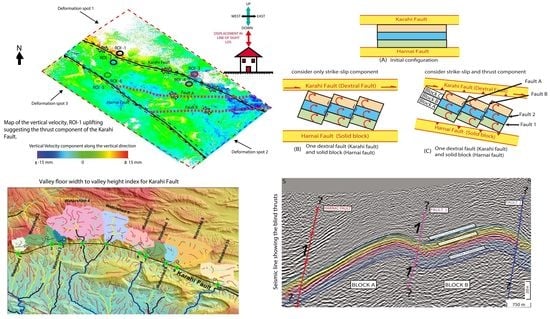
Figure 9D illustrates the vertical component of movement as either subsidence or uplift. The uplift is characterized by positive values (red color), while subsidence is characterized by negative values (blue color). According to Figure 9D, for deformation spot 1, there is a slight uplift on the northwest portion shown as red. This uplift is shown on the plot of ROI-1 with 10 mm movement rate (Figure 9D). The plot of ROI-2 shows stable movement throughout the observation time (Figure 9D). These two ROI-1 and ROI-2 show the northern and southern parts of the Karahi Fault, respectively. This could provide information about the thrust component of the Karahi Fault. Additionally, the eastern part of deformation spot 1 shows a subsidence deformation zone that could explain the boundary of Fault A. The areas of ROI-5 and ROI-6 do not show any vertical displacement (Figure 9D).
4.2. Geophysical and Subsurface Investigation
Figure 2B shows the location of 2D seismic lines and one well in the study area. At the surface, unconsolidated alluvium and sediments of the Ghazij Formation are exposed. In order to understand subsurface stratigraphy and details of faulting, 10 seismic lines were interpreted, but only these three fault lines were illustrated in this paper (Figure 10, Figure 11 and Figure 12). Three of these lines show the Harnai fault and 3D and 2D surfaces generated using these 10 seismic lines and well data.
Figure 10 shows the 2D seismic interpretation of line ZRT04-02. For stratigraphic interpretation, Ziarat-01 well was tied to seismic line ZRT04-02 using the well to seismic tie function in Kingdom. The interpreted horizons were then transferred to other seismic lines for understanding structural complexity. Additionally, time to depth conversion was made by using well-log velocity information. Ziarat-01 well was drilled to the depth of 1050 m (Figure 10A). The well data show that the first 414 m represent the Eocene Ghazij Shale. The Paleocene Dunghan Limestone follows with a thickness of 254 m. Other stratigraphic intervals drilled include Moro, Mughal Kot, Parh, Upper Goru Formations that are Late Cretaceous in age, and the Lower Goru and Sembar Formation of the early Cretaceous. The deepest stratigraphic horizon drilled in Ziarat-01 well was the Middle Jurassic Chiltan Formation at a depth of 833 m.
The Moro Formation consists of 27 m-thick sandstone, while Mughal Kot Formation comprises interbedded shale and sandstone with some limestone intervals. The Parh Formation consists of White Limestone. The Goru Formation contains an assortment of lithologies, including marl, shale, limestone, and quartzose sandstone. The succeeding formation, the Sembar Formation, consists mainly of shale. The total thickness of these formations is 165 m (from Moro to Sembar Formation).
At the top of Dungan Limestone, the Moro and the Chiltan formations show strong reflectors on the seismic section (Figure 10A–D) that provide reliable interpretation for seismic lines and also make a straightforward correlation between each seismic line. However, other formation tops cannot be identified except for these three formations due to the low vertical resolution of these lines. Therefore, Mughal Kot, Parh, Lower and Upper Goru, and Sembar formations tops have not been illustrated in the seismic section (Figure 10).
The 3D and 2D perspectives of the tops of the Dungan, Moro, Chiltan formations, newly identified two blind thrusts, and Harnai Fault are displayed in Figure 12 and Figure 13. An anticlinal structure can be seen at the location of the Ziarat-01 well. This elliptical anticline structure is east–west oriented, and its depth increases towards the east direction. This prospect has been drilled with the Ziarat Gas Field discovery in 2005 [27].
InSAR results presented in Figure 9 demonstrate that the Karahi fault is a right-lateral fault and Harnai Fault is a solid block or just a thrust component. The seismic result is most consistent with InSAR results, where the Harnai fault is interpreted showing possible thrust. Therefore, based on the new findings, we propose a revised kinematic model for this area. The area between the Harnai Fault and Fault 1 is interpreted as Block-A. The area between Fault 1 and Fault 2 is interpreted as Block-B, and the area between Fault 2 and the Karahi Fault is interpreted as Block-C. In the south part of the seismic line ZRT04-04, Harnai Fault is identified and interpreted as a thrust fault (Figure 11). While the south part of the Harnai Fault is described as a hanging wall, the north part is interpreted as a footwall. Two additional faults, Fault 1 and Fault 2, are also detected. Fault 1 and Fault 2 can be described as blind thrust faults because of the hanging wall (southernmost side) of both faults. A compression component can be seen. This compression is portrayed in the seismic section as an elevated section adjacent to the hanging attributes in Figure 10. These different types of attributes are used for the illustration of the Harnai Fault. Three different horizons are classified on the seismic line BOL98-11 with light blue, yellow, and dark blue colors (Figure 12). The light blue color represents the top of the Dunghan Formation. The yellow color shows the top of the Moro Formation and the dark blue color illustrates the Chiltan Formation. Data from the Ziarat-01 well show that tops of both Dunghan and Moro formations can easily be detected in the seismic lines. Three different thrust faults are detected on this seismic line. The Harnai Fault is observed in the southern part of the seismic line.
4.3. Tectonic Geomorphology
To determine the role of recent tectonic activities on the drainage basins, hypsometric integral and valley floor width to height indices were calculated for all the watersheds across the Harnai and Karahi faults. Fourteen watersheds for the Harnai fault and 10 watersheds for the Karahi fault were selected to illustrate hypsometric curves (Figure 14 and Figure 15). While the average hypsometric integral ratio of watersheds for the Karahi Fault is 0.469 (Table 3), the average hypsometric integral for the Harnai Fault is 0.392 (Table 4). Analysis of the hypsometric integral is based upon digital elevation models and utilization of all watershed results shown in Table 3 and Table 4. Overall, higher values of the hypsometric integral are illustrated by a convex shape curve indicating a young stage of drainage evolution. These values are generally > 0.5. Intermediate values tend to be both concave and convex, displayed by an S-shaped curve with values ranging between 0.4 and 0.5, which is considered a mature basin. Lastly, lower values < 0.4 tend to have concave-shaped curves (Figure 7B).
In general, lower values describe older eroded landscapes in the late stages of geomorphic evolution. However, higher values of the index usually indicate that less of the uplands has been eroded and may indicate a younger landscape, perhaps generated by active tectonic processes. Therefore, watersheds related to the Karahi fault, which demonstrated a majority of “S”-shaped curves contain both young and mature basins. However, watersheds relating to Harnai Fault demonstrate a majority of concave curve shapes, indicating a mature basin (Figure 16).
A total of 26 watersheds were extracted and analyzed for their Valley Floor Width-to-Height Ratio. Ten watersheds were evaluated for their Vf value for the Harnai Fault and show an average value of 0.83, indicating a relatively moderate level of tectonic activity. For the Karahi Fault, 14 watersheds were analyzed and they show an average Vf value of 0.32, which is quite low in comparison to the Harnai Fault and represents high tectonic activity in this area.
5. Discussion
The western part of the Suleiman Fold Belt is a structurally complex area represented by a series of thrust and strike-slip faults with varying geometry and kinematics. Previous researchers have made a few efforts in an attempt to describe the sense of movement of the parallel, NW–SE trending Karahi and Harnai faults, and interpret the style of deformation.
Our InSAR results, seismic interpretation, geomorphological indices, and published GNSS velocities suggest that shearing has played a significant role in the deformation of the western Suleiman Fold Belt (Figure 9). The shear zone has undergone simple shear deformation (Figure 17). This may be related to the oblique convergence of the Indian plate moving at a direction of N05E relative to the Eurasian plate [42,43]. Oblique convergent boundaries have resulted in a 3D distribution of deformation (simultaneous interaction between contractional and strike-slip motion), observed in the shear zone of the western Suleiman fold belt [44,45]. Our results agree with Teyssier’s strike-slip partitioned transpression model shown in Figure 17 [44]. The model is effective in understanding the relationship between plate motion, instantaneous strain axes, and degree of strike-slip partitioning.
The shear zone is strongly affected by the movements along the Karahi and Harnai faults. While the Karahi Fault displays a sense of strike-slip and thrust motions on InSAR results (Figure 9), the Harnai Fault only shows thrust motion on seismic profiles (Figure 10, Figure 11 and Figure 12).
The compressional forces perpendicular to the Harnai and Karahi faults seem to dominate when compared to lateral motions along these faults. As a result of the shearing of this zone, possible left-lateral strike-slip movement (Fault A and Fault B) compartmentalized this zone into distinct blocks such as Block A and Block B. If the Karahi Fault is interpreted as a right-lateral strike-slip fault, then Harnai Fault would be considered a solid block, and the shear zone of Fault A and Fault B can be interpreted as left-lateral strike-slip faults. These interpretations support the “bookshelf model” with the interpretation of shearing in this region having a clockwise rotation (Figure 17).
The bookshelf model, proposed initially by Mandl [46], is the behavior of parallel faults that relate to a horizontal stack of books being displaced and consequently named ‘bookshelf faulting’ [46,47,48]. Mandl [46] described two basic modes of mechanism: the “dilational” mode and the “domino” mode. While he proposed the dilational mode as two parallel faults that tend to open up and possibly become paths for fluid migration, the domino mode is described as reclining faults that remain closed. In both scenarios, the formation and rotation of the faults may occur in one tectonic event [46]. The bookshelf model is generally applied to describe the antithetic accommodation of deformation affected by direct shear.
In conforming to the model, the southern block of the Harnai Fault is assumed to be fix and rigid. InSAR and seismic results support this assumption. The average right-lateral movement of the Karahi Fault is at a rate of around 15 mm/yr (Figure 9B), while the Harnai Fault does not show strike-slip movement on InSAR datasets (Figure 9A–C). Since the Karahi Fault has higher displacement than the Harnai Fault, the net movement should result in a fixed southern block. The interpretation of this study is similar to the rotational block model suggested by Szeliga [13] and Huang et al. [18]. According to this model, the shear zone of the western Suleiman Fold Belt is compartmentalize into blocks that have rotated in a clockwise rotation due to right-lateral shear [13]. One distinct characteristic of this model is the presence of parallel strike-slip faults (Fault 1 and Fault 2) which resemble a horizontal stack of books being displaced and hence the name “bookshelf faulting” (Figure 18). Anticlinal structures are visible on the surface, indicating an uplift on the InSAR dataset between Karahi and Harnai faults (Figure 18D). Another embedded anticlinal structure was observed on the seismic section in the northern portion of the study area. These actively deforming anticlines mostly have a northeast–southwest direction, suggesting the “bookshelf model” with clockwise rotation.
Seismic data allowed us to understand the geometry of Harnai Fault in the Ziarat Block. Jadoon et al. [27] recognize the structures in the Ziarat Block as an in-sequence passive roof duplex and out of sequence deformation with the segmentation of the duplex structures. While Jadoon et al. [27] show Fault 1 and Fault 2 as blind thrust faults, they did not depict the Harnai Fault in their interpretation. They also describe Fault 2 as the main detachment fault. However, in this work, we described all these faults (Harnai, Fault 1, and Fault 2) as blind thrust faults with no surface trace or disruption. The area between the Harnai Fault and Fault 1 illustrates Block A and the area between Fault 1 and Fault 2 is interpreted as Block B. These block structures and existing faults may also indicate the presence of the “bookshelf model” (Figure 18).
Hypsometric integral results in this study, following Perez’s [37] and El Hamdouni’s [40] classifications, indicate that the Harnai Fault is comparatively less active or is in a more mature stage than the Karahi Fault, which is tectonically more active (Table 3 and Table 4). In addition, the northern part of the Karahi Fault can be interpreted as having relatively high tectonic activity due to the lower Vf values. In contrast, the southern part of the Harnai Fault is interpreted as having lower tectonic activity because of higher Vf values (Table 3 and Table 4). Overall, both the Hypsometric integral and Valley Floor Width to Height Ratio results support the InSAR findings, suggesting higher displacement along the Karahi Fault than the Harnai Fault.
6. Conclusions
This study integrates seismic reflection, InSAR SBAS analysis and geomorphological analysis to picture subsurface geometry and map surface deformation in the western part of the Suleiman Fold-Thrust Belt along the Harnai and Karahi Faults. Our findings are summarized below;
- The Karahi Fault is a right-lateral strike-slip fault, confirmed by the ascending and descending path geometry of Sentinel-1 datasets. This conclusion is also supported by the GNSS dataset. This right-lateral movement of the Karahi Fault could potentially be the reason for the clockwise movement.
- An average right-lateral movement of ~15 mm/yr is calculated for Karahi Fault for descending and ~10 mm/yr for ascending track geometries, respectively. Also, the SANJ GNSS station close to the Karahi Fault shows the 20 mm/yr rate of displacement in the southeast direction.
- No displacement is observed on the velocity map for the Harnai Fault and is interpreted as an aseismic.
- The 2D seismic interpretation shows the thrust component of the Harnai Fault. However, the lateral component of motion was not identified on the 2D seismic for both faults.
- Fault A and B observed on the seismic sections might be evidence of the compartmentalization between the Karahi and Harnai faults, and we interpreted this to be best explained by a “bookshelf faulting” model.
- Folds identified both in the subsurface and surface indicate an active uplift on the InSAR dataset.
- Both the calculated geomorphological indices, i.e., HI and Vf indicate relatively high tectonic activity associated with the Karahi Fault and low tectonic activity along the Harnai fault.
Author Contributions
Conceptualization and writing original draft preparation by S.O.K. and S.D.K., data processing by S.O.K.; I.A.A. helped in tectonic model and review and editing; E.O. supervised geomorphic indices calculation and interpretation; S.D.K. supervision and funding acquisition S.D.K., K.A.Q. obtained 2D seismic data and drafted two figures. All authors have read and agreed to the published version of the manuscript.
Funding
GeoRS Lab directed by S.D.K. supported software/hardware. S.O.K was funded for MS research by Turkish Ministry of National Education with the awarded scholarship of Selection and Placement of Students to be sent abroad for graduate studies (YLSY).
Acknowledgments
S.O.K. thanks Muhammad Qasim, Aydin Shahtakhtinskiy and GeoRS Lab for their help and discussions on various aspects of this research. The author would like to acknowledge support from the General Directorate of Mineral Research and Exploration (MTA), Remote Sensing and GIS Division, Department of Geological Research. The author would also like to thank Derman Dondurur, Orhan Atgin and Dokuz Eylul Unversity SeisLab for their support. Directorate General of Petroleum Concessions, Pakistan, is acknowledged for providing the well and seismic data. TanDEM-X provided by German Aerospace Center (DLR).
Conflicts of Interest
The authors declare no conflict of interest.
References
- Jadoon, I.A.K.; Lawrence, R.D.; Lillie, R.J. Seismic data, geometry, evolution, and shortening in the active Sulaiman fold-and-thrust belt of Pakistan, southwest of the Himalayas. Am. Assoc. Pet. Geol. Bull. 1994, 78, 758–774. [Google Scholar]
- Yeats, R.S.; Lawrence, R.D. Tectonics of the Himalayan thrust belt in northern Pakistan. In Marine Geology and Oceanography of the Arabian Sea and Coastal Pakistan; Van Nostrand Reinhold: New York, NY, USA, 1984; pp. 177–198. [Google Scholar]
- Zhang, P.; Shen, Z.-K.; Wang, M.; Gan, W.; Bürgmann, R.; Molnar, P.; Wang, Q.; Niu, Z.; Sun, J.; Wu, J.; et al. Continuous de-formation of the Tibetan Plateau from global positioning system data. Geology 2004, 32, 809–812. [Google Scholar] [CrossRef]
- Lave, J.; Avouac, J.P. Active folding of fluvial terraces across the Siwaliks Hills, Himalayas of central Nepal. J. Geophys. Res. Solid Earth 2000, 105, 5735–5770. [Google Scholar] [CrossRef] [Green Version]
- Burgess, W.P.; Yin, A.; Dubey, C.S.; Shen, Z.-K.; Kelty, T.K. Holocene shortening across the Main Frontal Thrust zone in the eastern Himalaya. Earth Planet. Sci. Lett. 2018, 357, 152–167. [Google Scholar] [CrossRef]
- Malik, J.N.; Nakata, T. Active faults and related Late Quaternary deformation along the Northwestern Himalayan Frontal Zone, India. Ann. Geophys. 2003, 46, 917–936. [Google Scholar]
- Abir, I.A.; Khan, S.D.; Ghulam, A.; Tariq, S.; Shah, M.T. Active tectonics of western Potwar Plateau-Salt Range, northern Pakistan from InSAR observations and seismic imaging. Remote Sens. Environ. 2015, 168, 265–275. [Google Scholar] [CrossRef] [Green Version]
- Jouanne, F.; Munawar, N.; Mugnier, J.-L.; Ahmed, A.; Alam Awan, A.; Bascou, P.; Vassallo, R. Seismic coupling quantified on inferred decollements beneath the western syntaxis of the Himalaya. Tectonics 2020, 39, 1–20. [Google Scholar] [CrossRef]
- Marshak, S. Salients, recesses, arcs, Oroclines, and SyntaxesA review of ideas concerning the formation of map-view curves in fold-thrust belts. AAPG Mem. 2004, 82, 131–156. [Google Scholar]
- Kumar, M.; Ravi, D.; Mishra, C.; Singh, B. Lithosphere, crust and basement ridges across Ganga and Indus basins and seismicity along the Himalayan front, India and Western Fold Belt, Pakistan. J. Asian Earth Sci. 2013, 75, 126–140. [Google Scholar] [CrossRef]
- Bilham, R.; Ambraseys, N. Apparent Himalayan slip deficit from the summation of seismic moments for Himalayan earthquakes, 1500–2000. Curr. Sci. 2005, 88, 1658–1663. [Google Scholar]
- Reynolds, K.; Copley, A.; Hussain, E. Evolution and dynamics of a fold-thrust belt: The Sulaiman Range of Pakistan. Geophys. J. Int. 2015, 201, 683–710. [Google Scholar] [CrossRef] [Green Version]
- Szeliga, W.M. Historical and Modern Seismotectonics of the Indian Plate with an Emphasis on Its Western Boundary with the Eurasian Plate. Ph.D. Thesis, Department of Geological Sciences, University of Colorado, Boulder, CO, USA, 2010. [Google Scholar]
- Szeliga, W.; Bilham, R.; Kakar, D.M.; Lodi, S.H. Interseismic strain accumulation along the western boundary of the Indian subcontinent. J. Geophys. Res. 2012, 117. [Google Scholar] [CrossRef] [Green Version]
- Crupa, W.E.; Khan, S.D.; Huang, J.; Khan, A.S.; Kasi, A. Active tectonic deformation of the western Indian plate boundary: A case study from the Chaman Fault System. J. Asian Earth Sci. 2017, 147, 452–468. [Google Scholar] [CrossRef]
- Fattahi, H.; Amelung, F. InSAR observations of strain accumulation and fault creep along the Chaman Fault system, Pakistan and Afghanistan. Geophys. Res. Lett. 2016, 43, 8399–8406. [Google Scholar] [CrossRef] [Green Version]
- Huang, J.; van Nieuwenhuise, D.; Khan, S.D.; Khan, A.S. Reflection seismic, gravity, magnetic, and InSAR analysis of the Chaman Fault in Pakistan. Arab. J. Geosci. 2020, 13, 1–14. [Google Scholar] [CrossRef]
- Huang, J.; Khan, S.D.; Ghulam, A.; Crupa, W.; Abir, I.A.; Khan, A.S.; Kakar, D.M.; Kasi, A.; Kakar, N. Study of subsidence and earthquake swarms in the western Pakistan. Remote Sens. 2016, 8, 956. [Google Scholar] [CrossRef] [Green Version]
- Qureshi, K.A.; Khan, D.S. Active Tectonics of the Frontal Himalayas: An Example from the Manzai Ranges in the Recess Setting, Western Pakistan. Remote Sens. 2020, 12, 3362. [Google Scholar] [CrossRef]
- Li, Y.; Shan, X.; Qu, C.; Liu, Y.; Han, N. Crustal Deformation of the Altyn Tagh Fault Based on GPS. J. Geophys. Res. Solid Earth 2018, 123, 10309–10322. [Google Scholar] [CrossRef]
- Fielding, E.; Simons, M.; Stephenson, O.; Zhong, M.; Yun, S.H.; Liang, C.; Sangha, S.; Ross, Z.E.; Huang, M.H.; Brooks, B.A. Geodetic Imaging of the Coseismic and Early Postseismic Deformation from the 2019 M w 7.1 and M w 6.4 Ridgecrest Earthquakes in California with SAR. Earth Space Sci. Open Arch. ESSOA 2019. [Google Scholar] [CrossRef]
- Xue, L.; Schwartz, S.; Liu, Z.; Feng, L. Interseismic megathrust coupling beneath the Nicoya Peninsula, Costa Rica, from the joint inversion of InSAR and GPS data. J. Geophys. Res. Solid Earth 2015, 120, 3707–3722. [Google Scholar] [CrossRef] [Green Version]
- Bannert, D.; Cheema, A.; Ahmed, A.; Schäffer, U. The structural development of the western fold thrust belt, Pakistan. Geol. Jahrbuch Reihe 1992, 80, 1–60. [Google Scholar]
- Pinel-Puysségur, B.; Grandin, R.; Bollinger, L.; Baudry, C. Multifaulting in a tectonic syntaxis revealed by InSAR: The case of the Ziarat earthquake sequence (Pakistan). J. Geophys. Res. Solid Earth 2014, 119, 5838–5854. [Google Scholar] [CrossRef]
- Quittmeyer, R.C.; Kafka, A.L. Constraints on plate motions in southern Pakistan and the Northern Arabian Sea from the focal mechanisms of small earthquakes. J. Geophys. Res. 1984, 89, 2444–2458. [Google Scholar] [CrossRef]
- Maldonado, F.; Mengal, J.M.; Khan, S.H.; Warwick, P.D. Summary of the Stratigraphy and Structural Elements Related to Plate Convergence of the Quetta-Muslim Bagh-Sibi Region, Balochistan, West-Central Pakistan; US Department of the Interior, US Geological Survey: Liston, VA, USA, 2011. [CrossRef]
- Jadoon, I.A.K.; Ding, L.; Nazir, J.; Idrees, M.; Jadoon, S.R.K. Structural interpretation of frontal folds and hydrocarbon exploration, western sulaiman fold belt, Pakistan. Mar. Pet. Geol. 2020, 117, 104380. [Google Scholar] [CrossRef]
- Altamimi, Z.; Collilieux, X.; Legrand, J.; Garayt, B.; Boucher, C. ITRF2005: A new release of the International Terrestrial Reference Frame based on time series of station positions and Earth Orientation Parameters. J. Geophys. Res. Solid Earth 2007, 112, 1–19. [Google Scholar] [CrossRef] [Green Version]
- Humayon, M.; Lillie, R.J.; Lawrence, R.D. Structural interpretation of the eastern Sulaiman foldbelt and foredeep, Pakistan. Tectonics 1991, 10, 299–324. [Google Scholar] [CrossRef]
- Banks, C.J.; Warburton, J. Passive-roof’duplex geometry in the frontal structures of the Kirthar and Sulaiman mountain belts, Pakistan. J. Struct. Geol. 1986, 8, 229–237. [Google Scholar] [CrossRef]
- Jadoon, S.U.R.K.; Ding, L.; Jadoon, I.A.K.; Baral, U.; Qasim, M.; Idrees, M. Interpretation of the Eastern Sulaiman fold-and-thrust belt, Pakistan: A passive roof duplex. J. Struct. Geol. 2019, 126, 231–244. [Google Scholar] [CrossRef]
- Rucci, A.; Ferretti, A.; Guarnieri, A.M.; Rocca, F. Sentinel 1 SAR interferometry applications: The outlook for sub millimeter measurements. Remote Sens. Environ. 2012, 120, 156–163. [Google Scholar] [CrossRef]
- Berardino, P.; Fornaro, G.; Lanari, R.; Sansosti, E. A new algorithm for surface deformation monitoring based on small baseline differential SAR interferograms. IEEE Trans. Geosci. Remote Sens. 2002, 40, 2375–2383. [Google Scholar] [CrossRef] [Green Version]
- Strahler, A.N. Quantitative analysis of watershed geomorphology. Eos Trans. Am. Geophys. Union 1957, 38, 913–920. [Google Scholar] [CrossRef] [Green Version]
- Keller, E.A.; Pinter, N. Active Tectonics, Earthquakes, Uplift and Landscape; Prentice Hall: Hoboken, NJ, USA, 2002. [Google Scholar]
- Dikpal, R.L.; Renuka Prasad, T.J.; Satish, K. Evaluation of morphometric parameters derived from Cartosat-1 DEM using remote sensing and GIS techniques for Budigere Amanikere watershed, Dakshina Pinakini Basin, Karnataka, India. Appl. Water Sci. 2017, 7, 4399–4414. [Google Scholar] [CrossRef] [Green Version]
- Pérez-Peña, J.V.; Azañón, J.M.; Booth-Rea, G.; Azor, A.; Delgado, J. Differentiating geology and tectonics using a spatial autocorrelation technique for the hypsometric integral. J. Geophys. Res. Earth Surf. 2009, 114, 1–15. [Google Scholar] [CrossRef]
- Pike, R.J.; Wilson, S.E. Elevation-relief ratio, hypsometric integral, and geomorphic area-altitude analysis. Bull. Geol. Soc. Am. 1971, 82, 1079–1084. [Google Scholar] [CrossRef]
- Bull, W.B. Tectonic Geomorphology of the Mojave Desert: US Geological Survey Contract Report 14-08-001-G-394; Office of Earthquakes, Volcanoes, and Engineering: Menlo Park, CA, USA, 1977; p. 188.
- El Hamdouni, R.; Irigaray, C.; Fernández, T.; Chacón, J.; Keller, E.A. Assessment of relative active tectonics, southwest border of the Sierra Nevada (southern Spain). Geomorphology 2008, 96, 150–173. [Google Scholar] [CrossRef]
- Silva, P.G.; Goy, J.L.; Zazo, C.; Bardají, T. Faulth-generated mountain fronts in southeast Spain: Geomorphologic assessment of tectonic and seismic activity. Geomorphology 2003, 50, 203–225. [Google Scholar] [CrossRef]
- Abdel-Gawad, M. Wrench movements in the Baluchistan Arc and relation to Himalayan-Indian Ocean Tectonics. Geol. Soc. Am. Bull. 1971, 82, 1235–1250. [Google Scholar] [CrossRef]
- Haq, S.S.B.; Davis, D.M. Oblique convergence and the lobate mountain belts of western Pakistan. Geology 1997, 25, 23–26. [Google Scholar] [CrossRef]
- Teyssier, C.; Tikoff, B.; Markley, M. Oblique plate motion and continental tectonics. Geology 1995, 23, 447–450. [Google Scholar] [CrossRef]
- Fossen, H.; Tikoff, B. The deformation matrix for simultaneous simple shearing, pure shearing and volume change, and its application to transpression-transtension tectonics. J. Struct. Geol. 1993, 15, 413–422. [Google Scholar] [CrossRef]
- Mandl, G. Tectonic deformation by rotating parallel faults—The bookshelf mechanism: Tectonophysics, v. 141. Tectonophysics 1987, 141, 277–316. [Google Scholar] [CrossRef]
- De Figueiredo, R.P.; Vargas , E.D.A., Jr.; Moraes, A. Analysis of bookshelf mechanisms using the mechanics of Cosserat generalized continua. J. Struct. Geol. 2004, 26, 1931–1943. [Google Scholar] [CrossRef]
- Zuza, A.V.; Yin, A. Continental deformation accommodated by non-rigid passive bookshelf faulting: An example from the Cenozoic tectonic development of northern Tibet. Tectonophysics 2016, 677, 227–240. [Google Scholar] [CrossRef] [Green Version]
Figure 1.
Shuttle Radar Topographic Mission (SRTM) DEM (30 m) showing the regional tectonics of the western Himalaya in Pakistan. The red box indicates the study area near the Sibi reentrant. Earthquakes with magnitude 5.0 or above are shown on the map (data source is USGS Earthquake Catalogue). The earthquakes’ years are highlighted to show highly devastating earthquakes from the last century. Map-view curvature of the SFTB is because of the Sibi and Tank reentrants. MBT, Main Boundary Thrust; JBF, Jhelum Basement Fault; SRT, Salt Range Thrust; SFTB, Suleiman Fold-Thrust Belt; GF, Ghazaband Fault; KR, Kirthar Ranges; OF, Ornachnal Fault; MSZ, Makran Subduction Zone.

Figure 3.
Map showing the structural subdivision of the SFTB into the eastern, central, and western Ranges. The black rectangle indicates the satellite track (Sentinel-1A). Earthquakes with a magnitude greater than 5 and their focal mechanism solution derived from USGS are plotted to show their distribution across the SFTB [26]. A high density of earthquakes is plotted in the western Suleiman near to Quetta Syntaxis/Sibi reentrant. The foreland propagation of the deformation front is also prominent. SR, Suleiman Ranges.

Figure 4.
(A) The geological map of the western Suleiman Fold Belt showing both structural and stratigraphic elements. Dotted lines A-A’ and B-B’ show the location of the structural cross-section in (B,C). (B) Surface topography and structural cross-section across the Harnai and Karahi faults. The yellow rectangle shows the seismic location and coverage. (C) Structural cross-section in the eastern part of the study area showing the fault-related folds in the form of duplexes. (B,C) are modified after Maldonado et al. [26] and Jadoon et al. [31].

Figure 5.
Interferometric Synthetic Aperture Radar processing workflow using small baseline subset technique.
Figure 5.
Interferometric Synthetic Aperture Radar processing workflow using small baseline subset technique.

Figure 6.
SAR interferograms showing spatial-temporal baseline distribution, where each acquisition is represented by a diamond associated with an ID number; the yellow diamond represents reference acquisition and green diamond represents the secondary time position plot of all interferograms generated by S1 data showing a perpendicular baseline between different image’s acquisition according to their relative position.

Figure 8.
Measurement of valley floor width to height ratio.

Figure 9.
Image showing displacement in which red color indicates movement towards the satellite (LOS direction) or uplift, and the blue color indicates movement away from satellite or subsidence. The graph shows the time series for three regions of interest (mm). (A) Displacement map and time series of the descending track geometry. (B) Displacement map and time series of the ascending track geometry. (C) Map of horizontal velocity component corresponding to the east–west direction and time series. The east direction is characterized by positive values (red color); the west direction is represented by negative values. (D) Map of the vertical velocity component that corresponds to uplift/subsidence (up/down) direction and time series. The uplift is characterized by positive values (red color) while negative values characterize subsidence.


Figure 10.
Interpretation of seismic line ZRT04-02 seismic (A) part of ZRT04-02 seismic section and summary of information of Ziarat-01 well. (B–D) show the seismic attributes with Pseudo-relief, Average Energy, and Trace Envelope, respectively. (E) The location of the seismic section ZRT04-02 and well. The color bar shows the elevation (meters). The blue rectangle represents the area of the seismic section evaluated in (A).

Figure 11.
Interpretation of seismic line ZRT04-04. (A) The red dash line box shows the location of the Harnai Fault. (B) shows the model that extracts from the seismic section. (C–G) show the seismic attributes with Pseudo-relief (B), Average Energy (D,E), and Trace Envelope (F,G), respectively. (H) represents the location of the seismic section BOL98-11 highlighted in red color. The color depicts elevation (meters).

Figure 12.
Interpretation of seismic line BOL98-11. (A) represents an interpretation of BOL98-11 seismic section. (B,C) show the seismic attributes with Envelope and Pseudo-relief, respectively. (D) shows the location of the seismic section BOL98-11, and the color bar shows the elevation.
Figure 12.
Interpretation of seismic line BOL98-11. (A) represents an interpretation of BOL98-11 seismic section. (B,C) show the seismic attributes with Envelope and Pseudo-relief, respectively. (D) shows the location of the seismic section BOL98-11, and the color bar shows the elevation.

Figure 13.
Formation tops of the Dunghan, Moro, and Chiltan Formation. (A,C,E) show a 2D depth contour map of the Dunghan Formation, Moro Formation, and Chiltan Formation, respectively. The ages of these formations are Paleocene, Late/Early Cretaceous, and Middle Jurassic, respectively. (B,D,F) show the 3D depth surface of the Dungan Formation, Moro Formation, and Chiltan Formation.

Figure 14.
Hillshade map with stream order for Karahi Fault. The colored areas show the watersheds numbered from 1 to 14, while the green circle represents the location of the pour points. The black lines with stars display the location of the Vf index.
Figure 14.
Hillshade map with stream order for Karahi Fault. The colored areas show the watersheds numbered from 1 to 14, while the green circle represents the location of the pour points. The black lines with stars display the location of the Vf index.

Figure 15.
Hillshade map with stream order for Harnai Fault. The colored areas show the watersheds numbered from 1 to 14. The black line with star displays the location of the Vf index.
Figure 15.
Hillshade map with stream order for Harnai Fault. The colored areas show the watersheds numbered from 1 to 14. The black line with star displays the location of the Vf index.

Figure 16.
Hypsometric curves for Karahi and Harnai Faults.

Figure 17.
Diagram showing the simple shear mechanism for the right lateral shear zone [44]. The Harnai fault block is assumed to be fixed, while the Karahi fault block is moving. Due to the shearing of the Karahi Fault, the block in-between developed faulted anticlines in the form of bookshelf faulting visible on the surface.

Figure 18.
A proposed kinematic model with 2D seismic interpretation. (A) Initial bookshelf model, (B) considering only strike-slip component (C) considering strike-slip and thrust component (D) seismic line BOL98-11 from Figure 12A.
Figure 18.
A proposed kinematic model with 2D seismic interpretation. (A) Initial bookshelf model, (B) considering only strike-slip component (C) considering strike-slip and thrust component (D) seismic line BOL98-11 from Figure 12A.


Table 1.
Sentinel-1A data specification. The product type is L1 single look complex (SLC) with ascending and descending geometry and interferometric wide swath beam mode (IW). The following acronyms were used in the table: polarization (Pol), incident (Inc), azimuth (Az), range (Rg), wavelength (WL), maximum perpendicular baseline (Bp) and maximum temporal baseline (Bt).
| Product Type | Mode | Pass | Pol. | Inc/Az Angle | Rg × Az Spacing (m) | WL (cm) | Path | Frame No. | Max Bp (%) | Max Bt (days) |
|---|---|---|---|---|---|---|---|---|---|---|
| S1-A | IW | Ascending /Descending | VH | 38/81 | 3.8 × 13.8 | 5.6 | 144/78 | 193/491 | 45 | 150 |
Table 2.
Classification of Vf index. High Vf values (greater than 1), depicted by a broad U-shaped valley, indicate lateral erosion because of the stability of the base level or tectonic quiescence. In contrast, low Vf values (less than 0.5), depicted by a V-shaped valley, indicate tectonic uplift. Vf values in between 0.5 and 1 are considered moderate level tectonic activity [39,40,41].
| Classification | Definition | Vf Values |
|---|---|---|
| Class–1 | Vf ≤ 0.5 | High level tectonic activity |
| Class–2 Class–3 | 1 > Vf > 0.5 Vf ≥ 1 | Moderate level tectonic activity Low level tectonic activity |
Table 3.
Hypsometric integral and VF values for Karahi Fault.
| Segments | Hypsometric Integral (Unit-Less) | HI Classification According to Perez | HI Classification According to El Hamdouni | Vf | Vf Classification |
|---|---|---|---|---|---|
| Watershed-1 Watershed-2 Watershed-3 Watershed-4 Watershed-5 Watershed-6 Watershed-7 Watershed-8 Watershed-9 Watershed-10 | 0.497 0.420 0.501 0.543 0.514 0.453 0.434 0.428 0.477 0.420 | Mature Basin Mature Basin Young Basin Young Basin Young basin Mature Basin Mature Basin Mature Basin Mature Basin Mature Basin | Medium Medium High High High Medium Medium Medium Medium Medium | 0.31 0.26 0.34 0.27 0.27 0.21 0.25 0.42 0.12 0.52 | High level tectonic activity High level tectonic activity High level tectonic activity High level tectonic activity High level tectonic activity High level tectonic activity High level tectonic activity High level tectonic activity High level tectonic activity Moderate level tectonic activity |
| Average | 0.469 | 0.32 |
Table 4.
Hypsometric integral and VF values for Harnai Fault.
| Segments | Hypsometric Integral (Unit-Less) | HI Classification According to Perez | HI Classification According to El Hamdouni | Vf | Vf Classification |
|---|---|---|---|---|---|
| Watershed-1 Watershed-2 Watershed-3 Watershed-4 Watershed-5 Watershed-6 Watershed-7 Watershed-8 Watershed-9 Watershed-10 Watershed-11 Watershed-12 Watershed-13 Watershed-14 | 0.469 0.331 0.359 0.316 0.427 0.447 0.383 0.287 0.479 0.374 0.418 0.330 0.405 0.470 | Mature Basin Mature Basin Mature Basin Mature Basin Mature Basin Mature Basin Mature Basin Mature Basin Mature Basin Mature Basin Mature Basin Mature Basin Mature Basin Mature Basin | Medium Low Low Low Medium Medium Low Low Medium Low Medium Low Medium Medium | 0.51 1.15 0.96 1.05 1.21 0.68 0.51 0.82 0.62 0.93 1.24 0.76 0.62 0.62 | Moderate level tectonic activity Low level tectonic activity Moderate level tectonic activity Low level tectonic activity Low level tectonic activity Moderate level tectonic activity Moderate level tectonic activity Moderate level tectonic activity Moderate level tectonic activity Low level tectonic activity High level tectonic activity Moderate level tectonic activity Moderate level tectonic activity Moderate level tectonic activity |
| Average | 0.392 | 0.83 |
Publisher’s Note: MDPI stays neutral with regard to jurisdictional claims in published maps and institutional affiliations. |
© 2021 by the authors. Licensee MDPI, Basel, Switzerland. This article is an open access article distributed under the terms and conditions of the Creative Commons Attribution (CC BY) license (https://creativecommons.org/licenses/by/4.0/).
Share and Cite
MDPI and ACS Style
Karaca, S.O.; Abir, I.A.; Khan, S.D.; Ozsayın, E.; Qureshi, K.A. Neotectonics of the Western Suleiman Fold Belt, Pakistan: Evidence for Bookshelf Faulting. Remote Sens. 2021, 13, 3593. https://doi.org/10.3390/rs13183593
AMA Style
Karaca SO, Abir IA, Khan SD, Ozsayın E, Qureshi KA. Neotectonics of the Western Suleiman Fold Belt, Pakistan: Evidence for Bookshelf Faulting. Remote Sensing. 2021; 13(18):3593. https://doi.org/10.3390/rs13183593
Chicago/Turabian StyleKaraca, Sukru O., Ismail A. Abir, Shuhab D. Khan, Erman Ozsayın, and Kamil A. Qureshi. 2021. "Neotectonics of the Western Suleiman Fold Belt, Pakistan: Evidence for Bookshelf Faulting" Remote Sensing 13, no. 18: 3593. https://doi.org/10.3390/rs13183593
Note that from the first issue of 2016, this journal uses article numbers instead of page numbers. See further details here.