Tighten the Bolts and Nuts on GPP Estimations from Sites to the Globe: An Assessment of Remote Sensing Based LUE Models and Supporting Data Fields

Abstract

Gross primary production (GPP) determines the amounts of carbon and energy that enter terrestrial ecosystems. However, the tremendous uncertainty of the GPP still hinders the reliability of GPP estimates and therefore understanding of the global carbon cycle. In this study, using observations from global eddy covariance (EC) flux towers, we appraised the performance of 24 widely used GPP models and the quality of major spatial data layers that drive the models. Results show that global GPP products generated by the 24 models varied greatly in means (from 92.7 to 178.9 Pg C yr⁻¹) and trends (from −0.25 to 0.84 Pg C yr⁻¹). Model structure differences (i.e., light use efficiency models, machine learning models, and process-based biophysical models) are an important aspect contributing to the large uncertainty. In addition, various biases in currently available spatial datasets have found (e.g., only 57% of the observed variation in photosynthetically active radiation at the flux tower locations was explained by the spatial dataset), which not only affect GPP simulation but more importantly hinder the simulation and understanding of the earth system. Moving forward, research into the efficacy of model structures and precision of input data may be more important for global GPP estimation.

1. Introduction

Terrestrial gross primary production (GPP) or the total photosynthetic uptake of carbon by plants plays a critical role in maintaining the global carbon balance between the biosphere and atmosphere. However, the estimation of terrestrial GPP by existing models remains highly uncertain, with global estimates ranging widely between 92.7 to 168.7 Pg C yr⁻¹ [1,2,3]. This large uncertainty poses a serious obstacle to quantifying and understanding the global carbon cycle [4]. It is broadly agreed that, to reduce the uncertainty of GPP estimation and advance carbon cycle science, it is crucial to consider: (1) The impacts of model structure, (2) the determination of parameter values, and (3) the quality of data feeding in GPP models [5,6].

Model structure is considered one of the most important factors that affect model performance [7,8]. Yet, large structural differences can be observed among GPP models. For example, the fraction of photosynthetic active radiation (FPAR), an important parameter in the light use efficiency (LUE) models, has been treated in disparate ways, either approximated by the enhanced vegetation index (EVI) in the vegetation photosynthesis model (VPM) [9], as a linear function of normalized difference vegetation index (NDVI) in the eddy covariance-light use efficiency (EC-LUE) model [10], or as a nonlinear function of leaf area index (LAI) according to Beer’s Law, among others [11]. A similar situation exists for representing temperature stress (TS), water stress (WS), and their interactions among models. The moderate resolution imaging spectroradiometer (MODIS) model and the VPM model adopt a multiplicative structure to represent the collective influences of WS and TS on GPP [7,12]. The EC-LUE model, on the other hand, considers that the Liebig’s law is ecologically more reasonable in representing the effects of WS and TS [9].

The estimation of model parameters often affect the simulation accuracy of the model, thus rigorous model parameterization and calibration should be adopted in GPP modeling [13]. Variation in the values of the same biophysical parameters among different models is a major concern in GPP estimation. For example, the maximum light use efficiency (LUE(max)), a parameter used in LUE-based GPP models, represents the maximum efficiency of unit vegetation converting energy to photosynthates and therefore should be relatively stable [14]. However, it has taken many different values in LUE-based GPP models. In the MODIS model, LUE(max) values are biome-specific, varying from 0.604 to 1.259 g C MJ⁻¹ (Running et al., 2006), and similar approaches can be found in other models [15]. The EC-LUE model, on the other hand, takes a constant value at LUE(max) = 2.25 g C MJ⁻¹, that was derived from many flux tower observations, and the authors later advocated the use of different constant LUE(max) values for C3 and C4 plants [16]. However, another study has suggested that a fixed LUE(max) value would lead to increased GPP uncertainty [17]. An analysis of the parameters of the diagnostic carbon flux model (DCFM) showed that cross-site estimation improved the representativeness and robustness of parameter estimates [18]. Studies considering a wider number of flux towers are thus necessary for a more reliable tuning of GPP model parameters.

Regional to global simulations inevitably employ spatiotemporal data for initialization or as driving forces [19]. How spatial data products affect GPP simulation has rarely been assessed because users of the data products tend to take a leap of faith by assuming the quality of data has met the accuracy requirement and limited findings regarding the importance of data quality have been ignored frequently. For example, it was found that the widely used average of eight-days MODIS satellite FPAR data was unable to effectively reflect the reality [20]. Other studies have revealed that MODIS satellite FPAR products are systematically lower than ground-measured FPAR observations in winter and spring [21]. Clouds seriously affect satellite observations in humid regions such as the Amazon [22]. Even when applying a cloud correction by the CFMask algorithm [23] only 70% of PAR can be satisfactorily simulated [24]. Failure to reproduce the driving data of the models faithfully would affect the simulation and accuracy of GPP.

To address the three issues mentioned above and improve the estimation accuracy of GPP at a global scale, we comprehensively appraised the structure and performance of existing LUE models against GPP estimates from 151 eddy covariance (EC) flux towers worldwide, and assessed the impacts of using currently available data products on the estimates of global GPP using newly developed LUE models. The specific objectives were to: (1) Compare existing models and address model structure deficiency, if necessary, (2) find the optimal parameter values using GPP observed at the EC towers, (3) develop a new model to taking advantage of remote sensing (RS) data as directly as possible, reducing errors of intermediate data products and algorithms, (4) evaluate errors of spatial RS data and their impacts on GPP estimation, and (5) generate a new GPP model and subsequent global product, after correcting biases in spatial data layers.

2. Materials and Methods

In this study, using observations from global EC flux towers, we appraised 8 common satellite-data-based GPP models and the quality of major spatial data layers that drive the models. In order to utilize remote sensing data as directly as possible and minimize error propagation, 2 new GPP models were developed and compared with the 8 common satellite-data-based GPP models. Finally, 24 existing global GPP products, including the global GPP product generated from the new model that showed better performance, were compared and analyzed for similarity and differences.

2.1. Description of Existing GPP Models Used in this Study and the New Models

A total of 8 common satellite-data-based GPP models and 22 global GPP products were included in this study. The 8 existing models were the eddy covariance-light use efficiency (EC-LUE) model [9], the vegetation-indices (VI) model [25], the temperature-greenness (TG) model [26], the vegetation photosynthesis model (VPM) [11], the carbon fixation model (CFIX) model [27], the greenness-radiation (GR) model [28], the alpine vegetation (AVM) model [29], and the moderate resolution imaging spectroradiometer (MODIS) model [30]. At the site scale, we reproduced the 8 common satellite-data-based GPP models and compared them with the two new models in this study.

The two new models were adaptations of the EC-LUE model, which included corrections for cloudiness and CO₂ concentration, with two derivations for determining water stress: One from the evaporative fraction (i.e., the LUE-EF model) and another from the normalized difference water index (NDWI) (i.e., the LUE-NDWI model), as described below.

2.2. Description of the LUE-EF Model

This model was developed mainly based on the principles of the EC-LUE model [9]. Specifically, the regulation of water on GPP is represented by the evaporative fraction (EF), taking advantage of the newly available EF products [31]. In addition, two new modifiers of GPP were added to the original EC-LUE model. The first modifier considers the impact of cloudiness on GPP. The other modifier addresses the fertilization effect of increased CO₂ concentration in the atmosphere.

The LUE-EF model can be expressed as follows:

$$GPP =PAR\times FPAR\times F_{CI}\times F_{CO2}\times LU{E}_{\left(MAX\right)}\times \min \left(T_S,W_S\right)$$

(1)

where PAR is incident photosynthetic active radiation (MJ/m²) over a period of time; FPAR is the fraction of PAR absorbed by the vegetation; F_CI is the regulation of cloudiness on GPP; F_CO2 is the regulation scalar of atmospheric CO₂ concentration; LUE_(MAX) is the maximum light use efficiency; and T_S and W_S are regulation scalars respectively for temperature and water stress on GPP, from which the minimum value is taken, following the Leibig law [9], and the expression of Ts is the same as that of EC-LUE model. The determination of model parameters was done as:

• FPAR is in practice approximated by EVI [11], since photosynthetically active vegetation is estimated as a ratio α of EVI, set to be α = 1:

  $$FPA{R}_{EVI}=\alpha \times EVI;$$

  (2)
• Most previous models underestimates of GPP on cloudy days mainly because photosynthesis can be increased by diffuse radiation under cloudy conditions [6,32]. The regulating effect of cloud cover on GPP was expressed by a cloudiness index (CI) as follow:

  $$F_{CI}=a\times CI+b$$

  (3)

  where CI is the ratio of PAR to potential PAR (PPAR) [6], and PPAR is PAR that reaches the upper atmosphere. Using the FLUXNET2015 dataset, the coefficients were determined to be a (= 2.9) and b (= 1.2);
• For calculating the influence of atmospheric CO₂ on GPP, we employed the algorithm in the Frankfurt Biosphere Model (FBM):

  $$F_{CO2}=f\left(CO2,T\right)=\frac{CCL-∆\left(T\right)}{CCL+2∆\left(T\right)}$$

  (4)

  where CCL is the internal CO₂ concentration of leaves, and it assumed to be 70% of atmospheric CO₂ concentration [33]. Δ(T) is the CO₂ compensation point for gross photosynthesis and photorespiration at temperature T (°C) [34]:

  $$∆\left(T\right) = 40.6e^{\raisebox{1ex}{$\left(9.46\times \left(T-25\right)\right)$}\!\left/ \!\raisebox{-1ex}{$\left(T+273.2\right)$}\right.};$$

  (5)
• The regulation scalar of water on GPP, W_S, was expressed as the evaporative fraction (EF) of the total sensible and latent heat [9]:

  $$W_S=EF=\frac{LE}{ LE+H}$$

  (6)

  where LE is latent heat flux (W m⁻²), and H is sensible heat flux (W m⁻²).

2.3. Description of the LUE-NDWI Model

The LUE-NDWI model can be expressed as follows:

$$GPP =PAR\times FPAR\times F_{CI}\times F_{CO2}\times LU{E}_{\left(MAX\right)}\times \min \left(T_S,W_{S\_NDWI}\right).$$

(7)

It can be seen that the only difference between LUE-EF and LUE-NDWI is the expression for water stress. The NDWI, strongly related to vegetation water content [35,36], can be a very good proxy for vegetation water stress. In addition, NDWI data can be obtained through satellite observation directly and the EF obtained by calculating sensible heat and latent heat, cannot be directly observed. After examining measurements from many flux towers, we found that the following nonlinear function can be used to represent W_S, the regulation scalar of water stress on GPP, using NDWI:

$$W_{S\_NDWI}=a\ast {\left(-NDWI+0.5\right)}^b+\mathrm{c}.$$

(8)

Using the ‘nls’ method of parameter optimization adjustment, the coefficients were determined to be a (= 0.35), b (= 2.14), and c (= 0.086). The W_{S_NDWI} values vary between 0 and 1, with values beyond the bounds set to 0 or 1, respectively. The use of W_{S_NDWI} can be very convenient for applications from local to global scales as the NDWI fields can be directly derived from satellite observations.

2.4. Data for Evaluation of Models and Spatial Data Products

For an evaluation of models and remotely sensed data products, we used eddy covariance (EC) flux tower data from the FLUXNET2015 dataset (https://fluxnet.fluxdata.org) [37]. Our study included data from 151 EC tower sites that belonged to the following 12 terrestrial biomes: Croplands (CRO), closed Shrublands (CSH), deciduous broadleaf forest (DBF), deciduous needleleaf forest (DNF), evergreen broadleaf forest (EBF), evergreen needleleaf forest (ENF), grasslands (GRA), mixed forests (MF), open shrublands (OSH), savannas (SAV), permanent wetlands (WET), and woody savannas (WSA). We used two criteria to filter the data, following [6]: (1) If more than 20% of the data in a given year was missing, the whole year was discarded, and (2) after this first step of processing, EC-tower sites with records for less than two years were completely discarded. EC-towers details are in

Table A1. Eddy covariance (EC) sites information used for research, including site id (ID), site name (SITE), latitude and longitude (LAT, LON), and biome type (BIO). The asterisk is used to verify the model.

ID	SITE	LAT	LON	BIO
1	BE-Lon	50.5516	4.7461	CRO *
2	DE-Seh	50.8706	6.4497	CRO
3	FI-Jok	60.8986	23.5135	CRO
4	IT-CA2	42.3772	12.026	CRO *
5	US-CRT	41.6285	−83.347	CRO *
6	US-Lin	36.3566	−119.84	CRO
7	US-Tw3	38.1159	−121.65	CRO
8	US-Twt	38.1087	−121.65	CRO *
9	US-ARM	36.6058	−97.489	CRO *
10	US-Ne2	41.1649	−96.47	CRO
11	US-Ne3	41.1797	−96.44	CRO
12	DE-Kli	50.8931	13.5224	CRO
13	FR-Gri	48.8442	1.9519	CRO *
14	US-Ne1	41.1651	−96.477	CRO *
15	IT-Noe	40.6062	8.1512	CSH
16	US-KS2	28.6086	−80.672	CSH *
17	CA-Oas	53.6289	−106.2	DBF
18	CA-TPD	42.6353	−80.558	DBF
19	DE-Hai	51.0792	10.453	DBF *
20	DK-Sor	55.4859	11.6446	DBF *
21	FR-Fon	48.4764	2.7801	DBF
22	IT-CA1	42.3804	12.0266	DBF *
23	IT-CA3	42.38	12.0222	DBF
24	IT-Col	41.8494	13.5881	DBF
25	IT-Isp	45.8126	8.6336	DBF *
26	IT-Ro1	42.4081	11.93	DBF
27	IT-Ro2	42.3903	11.9209	DBF
28	PA-SPn	9.3181	−79.635	DBF *
29	US-Ha1	42.5378	−72.172	DBF *
30	US-MMS	39.3232	−86.413	DBF *
31	US-Oho	41.5545	−83.844	DBF
32	US-UMB	45.5598	−84.714	DBF *
33	US-UMd	45.5625	−84.698	DBF
34	US-WCr	45.8059	−90.08	DBF
35	ZM-Mon	−15.438	23.2528	DBF *
36	RU-SkP	62.255	129.168	DNF
37	AU-Cum	−33.615	150.724	EBF *
38	AU-Tum	−35.657	148.152	EBF
39	AU-Wac	−37.426	145.188	EBF *
40	AU-Whr	−36.673	145.029	EBF *
41	AU-Wom	−37.422	144.094	EBF
42	BR-Sa1	−2.8567	−54.959	EBF
43	BR-Sa3	−3.018	−54.971	EBF *
44	FR-Pue	43.7413	3.5957	EBF *
45	GF-Guy	5.2788	−52.925	EBF
46	IT-Cp2	41.7043	12.3573	EBF
47	IT-Cpz	41.7053	12.3761	EBF
48	MY-PSO	2.973	102.306	EBF
49	AU-ASM	−22.283	133.249	ENF *
50	CA-NS1	55.8792	−98.484	ENF
51	CA-NS2	55.9058	−98.525	ENF
52	CA-NS3	55.9117	−98.382	ENF *
53	CA-NS4	55.9144	−98.381	ENF
54	CA-NS5	55.8631	−98.485	ENF
55	CA-Obs	53.9872	−105.12	ENF *
56	CA-Qfo	49.6925	−74.342	ENF
57	CA-SF1	54.485	−105.82	ENF
58	CA-SF2	54.2539	−105.88	ENF *
59	CA-TP1	42.6609	−80.56	ENF
60	CA-TP2	42.7744	−80.459	ENF *
61	CA-TP3	42.7068	−80.348	ENF
62	CA-TP4	42.7102	−80.357	ENF *
63	CH-Dav	46.8153	9.8559	ENF *
64	CZ-BK1	49.5021	18.5369	ENF
65	DE-Lkb	49.0996	13.3047	ENF *
66	FI-Let	60.6418	23.9595	ENF
67	FR-LBr	44.7171	−0.7693	ENF *
68	IT-La2	45.9542	11.2853	ENF
69	IT-Ren	46.5869	11.4337	ENF *
70	IT-SR2	43.732	10.291	ENF *
71	RU-Fyo	56.4615	32.9221	ENF
72	US-Blo	38.8953	−120.63	ENF
73	US-GBT	41.3658	−106.24	ENF *
74	US-GLE	41.3665	−106.24	ENF *
75	US-Me2	44.4523	−121.56	ENF
76	US-Me3	44.3154	−121.61	ENF
77	US-Me5	44.4372	−121.57	ENF *
78	US-Me6	44.3233	−121.61	ENF
79	US-NR1	40.0329	−105.55	ENF *
80	US-Prr	65.1237	−147.49	ENF *
81	US-Wi4	46.7393	−91.166	ENF
82	US-Wi9	46.6188	−91.081	ENF *
83	AT-Neu	47.1167	11.3175	GRA *
84	AU-DaP	−14.063	131.318	GRA *
85	AU-Emr	−23.859	148.475	GRA *
86	AU-Rig	−36.65	145.576	GRA
87	CH-Cha	47.2102	8.4104	GRA *
88	CH-Fru	47.1158	8.5378	GRA
89	CH-Oe1	47.2858	7.7319	GRA
90	CN-Cng	44.5934	123.509	GRA *
91	CN-Dan	30.4978	91.0664	GRA *
92	CN-Du2	42.0467	116.284	GRA
93	CN-HaM	37.37	101.18	GRA
94	CZ-BK2	49.4944	18.5429	GRA *
95	DE-Gri	50.95	13.5126	GRA
96	DK-Eng	55.6905	12.1918	GRA *
97	DK-ZaH	74.4733	−20.55	GRA
98	IT-Tor	45.8444	7.5781	GRA
99	PA-SPs	9.3138	−79.631	GRA *
100	RU-Ha1	54.7252	90.0022	GRA *
101	RU-Tks	71.5943	128.888	GRA
102	US-AR1	36.4267	−99.42	GRA
103	US-AR2	36.6358	−99.598	GRA *
104	US-ARb	35.5497	−98.04	GRA
105	US-ARc	35.5465	−98.04	GRA *
106	US-Cop	38.09	−109.39	GRA
107	US-Goo	34.2547	−89.874	GRA
108	US-IB2	41.8406	−88.241	GRA *
109	US-SRG	31.7894	−110.83	GRA *
110	US-Var	38.4133	−120.95	GRA
111	US-Wkg	31.7365	−109.94	GRA *
112	BE-Bra	51.3076	4.5198	MF
113	BE-Vie	50.305	5.9981	MF *
114	CA-Gro	48.2167	−82.156	MF
115	CN-Cha	42.4025	128.096	MF *
116	US-Syv	46.242	−89.348	MF
117	CA-NS6	55.9167	−98.964	OSH *
118	CA-NS7	56.6358	−99.948	OSH *
119	CA-SF3	54.0916	−106.01	OSH
120	ES-Amo	36.8336	−2.2523	OSH
121	ES-LgS	37.0979	−2.9658	OSH *
122	US-SRC	31.9083	−110.84	OSH *
123	US-Whs	31.7438	−110.05	OSH
124	AU-Dry	−15.259	132.371	SAV
125	AU-GWW	−30.191	120.654	SAV *
126	CG-Tch	−4.2892	11.6564	SAV *
127	SD-Dem	13.2829	30.4783	SAV
128	SN-Dhr	15.4028	−15.432	SAV *
129	ZA-Kru	−25.02	31.4969	SAV *
130	AU-Fog	−12.545	131.307	WET
131	CN-Ha2	37.6086	101.327	WET *
132	CZ-wet	49.0247	14.7704	WET
133	DE-Akm	53.8662	13.6834	WET
134	DE-SfN	47.8064	11.3275	WET *
135	DE-Spw	51.8923	14.0337	WET
136	DE-Zrk	53.8759	12.889	WET
137	DK-NuF	64.1308	−51.386	WET *
138	DK-ZaF	74.4814	−20.555	WET
139	FI-Lom	67.9972	24.2092	WET *
140	SE-St1	68.3542	19.0503	WET
141	US-Atq	70.4696	−157.41	WET *
142	US-Ivo	68.4865	−155.75	WET *
143	US-Los	46.0827	−89.979	WET
144	US-Myb	38.0498	−121.77	WET
145	US-Tw1	38.1074	−121.65	WET *
146	US-WPT	41.4646	−82.996	WET
147	AU-Gin	−31.376	115.714	WSA
148	AU-How	−12.494	131.152	WSA *
149	AU-RDF	−14.564	132.478	WSA
150	US-SRM	31.8214	−110.87	WSA *
151	US-Ton	38.4316	−120.97	WSA *

* 12 terrestrial biomes: Croplands (CRO), closed Shrublands (CSH), deciduous broadleaf forest (DBF), deciduous needleleaf forest (DNF), evergreen broadleaf forest (EBF), evergreen needleleaf forest (ENF), grasslands (GRA), mixed forests (MF), open shrublands (OSH), savannas (SAV), permanent wetlands (WET), and woody savannas (WSA).

.

To simulate global GPP, the following spatial data products were used: (1) Meteorological data fields—radiation, air temperature, latent heat flux, and sensible heat flux—derived from the second Modern-Era Retrospective analysis for Research and Applications (MERRA-2), (2) MODIS satellite products including enhanced vegetation index (EVI) and normalized difference wetness index (NDWI), and (3) global atmospheric CO₂ concentration product from the Earth System Research Laboratory Global Monitoring Division (https://www.esrl.noaa.gov/gmd/dv/site/).

2.5. Evaluation of Spatial Data Products and Model Performance

In this study, data from FLUXNET eddy covariance flux tower sites were retained for analysis after data quality control. Half of the EC-towers were used for model calibration and the other half for validation. Values of model parameters were estimated using the Gauss–Newton algorithm for nonlinear optimization as implemented in the ’nls’ function in the R language (package ‘stats’ v3.6.1) [38]. The model uncertainty at the site scale was assessed using correlation coefficient (r), normalized root-mean-square error (RMSE), and standard deviation (SD) of predicted and observed values, displayed by the Taylor diagrams. In addition, the ability to capture temporal changes of GPP is essential for GPP models. The double mass curve (cumulative GPP predicted by model versus cumulative GPP observed at EC-towers) computed per site can reflect the ability of models to simulate the temporal changes of GPP, and the percentage bias (PB) of each site was counted [39].

It is critical that spatial data fields used to drive these models should represent the site-level conditions with high accuracy when these models are applied to estimate GPP at regional to global scales. In this study, the accuracy of spatial data products were evaluated against measurements collected at the flux tower sites. Specifically, orthogonal regressions were performed, comparing each of the spatial data products against their corresponding site-level measurements [40]. Their 1:1 correspondence and biases was assessed by a hypothesis tests (α = 0.05) of the regression coefficients, with null hypothesis being slope = 1 and intercept = 0 [41]. Orthogonal regression can take into account the errors of both the independent and dependent variables at the same time [42]. These analyses were conducted using the ‘scipy.stats’ and ‘odr’ packages in Python (v3) [43]. When generating global GPP products, the spatial data layers (i.e., uncorrected datasets) of driving variables were corrected according to the correction coefficients obtained at the site scale through orthogonal regression. The correction coefficients were the slope and intercept of linear regression between variable values measured at the flux towers and their equivalent from the spatial datasets.

Finally, we evaluated a total of 24 global GPP products: Two from this study (LUE-NDWI with uncorrected and corrected spatial datasets, respectively), and 22 products from TRENDY (http://dgvm.ceh.ac.uk/) [44] and other studies [3]. Specifically, the 22 global GPP products were EC-LUE, revised EC-LUE [6], MODIS [25], MOD17 C6 [45], PR [46], VPM [11], FLUXCOM-ANN, FLUXCOM-MARS, and FLUXCOM-RF from FLUXCOM [47], SVR [48], BESS [49], BEPS [50], and 10 TRENDY products. The performance of the LUE-EF model was not evaluated at a global scale because of the difficulty in estimating the water stress in the LUE-EF model (i.e., the evaporative fraction of net solar radiation), which cannot be readily derived from satellite observations. We analyzed the similarity and differences of the GPP products in magnitude, spatial patterns, and temporal trends.

3. Results

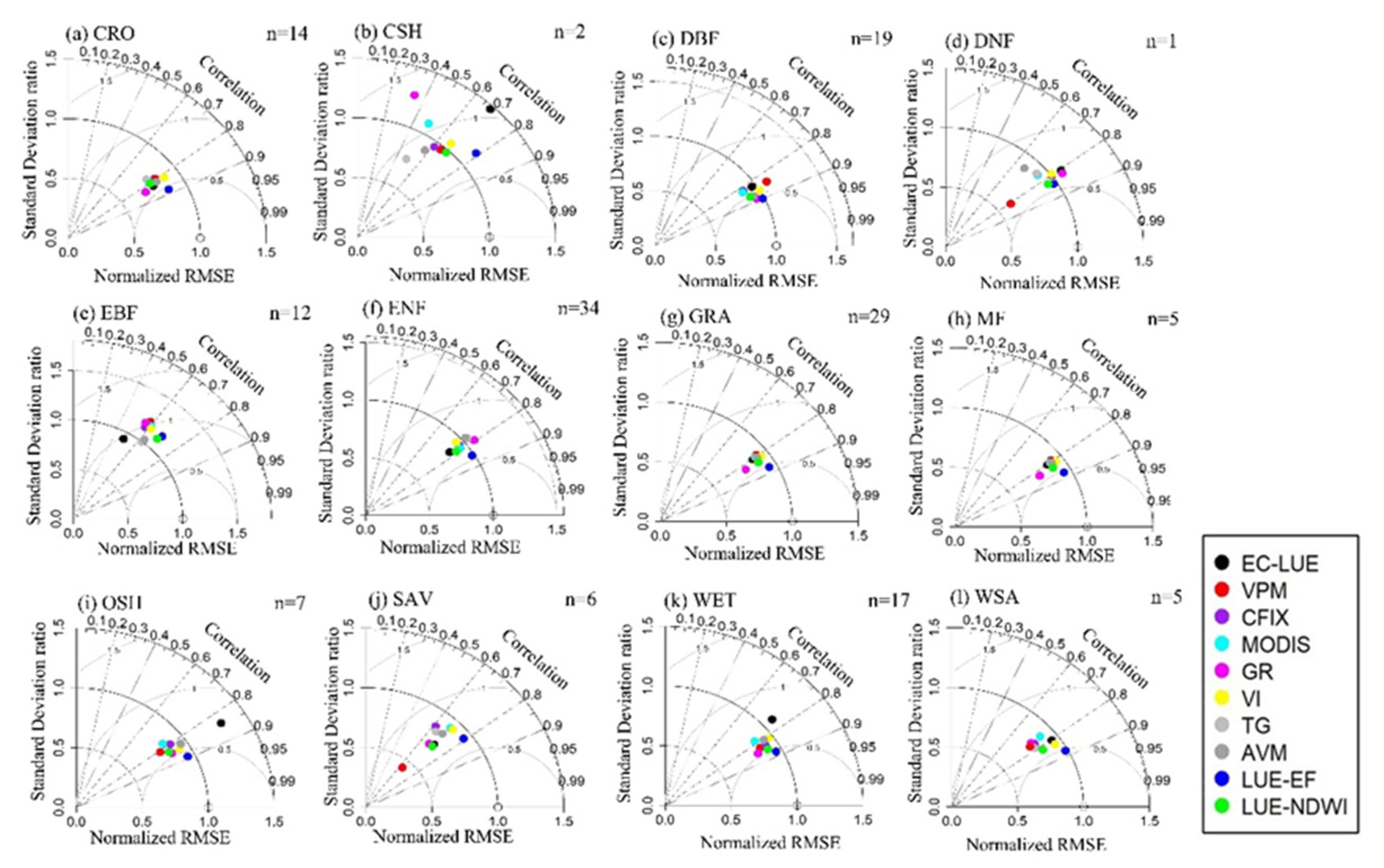
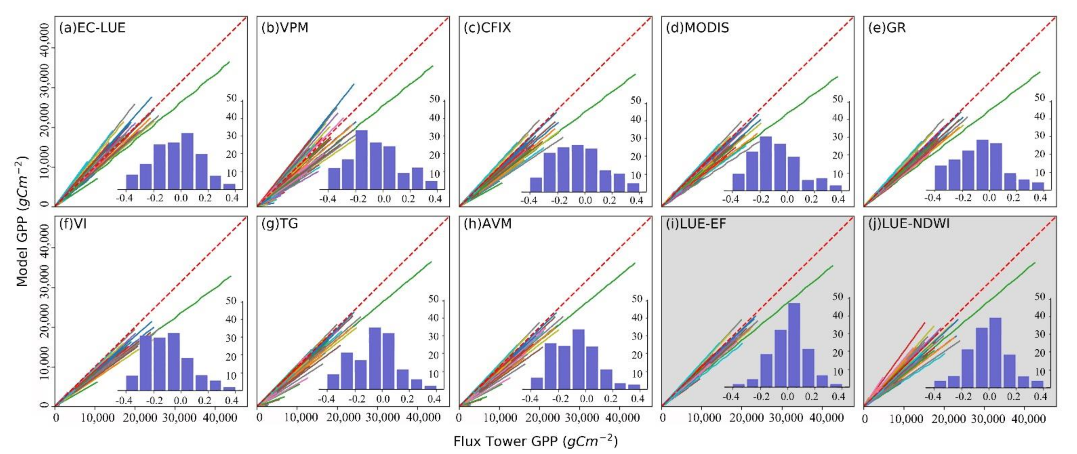
3.1. Comparison of Model Performance at the Site Scale

Globally among all the 10 models evaluated, the LUE-EF model had the highest correlation coefficient of r = 0.86, followed by the LUE-NDWI model with r = 0.82 (Figure 1a). The LUE-EF model had the smallest normalized RMSE (0.50), indicating that the difference between the LUE-EF model and EC-tower GPP was the smallest among all models. The LUE-NDWI model had the second smallest normalized RMSE (0.52). The normalized RMSE for the other models was larger than the two new models. Model LUE-EF simulated the amplitude of the variations close to the data amplitude of EC-towers (SD ratio = 0.93). When grouped by latitudinal zone (Figure 1b–e) the improvements of the new models were more apparent for tropical and northern temperate zones. In the temperate zones, the distribution of models in the Taylor diagram was relatively concentrated, whereas in the tropical and boreal areas there were larger differences among models. When grouped by biome (Figure A1), the new LUE-EF model showed advantages of fit in simulating daily GPP for most biomes, both in terms of correlation coefficients and RMSE. For example, correlation coefficients were highest for LUE-EF in deciduous broadleaved and evergreen needleleaf forests, wetlands, and grasslands (DBF, ENF, WET, and GRA), with LUE-NDWI being the second highest in the latter three of those. It is important to note that these biomes also have the largest number of EC-towers. It is relevant to note that many biomes are underrepresented in the current EC-tower network, such as closed shrublands or deciduous needle-leaved forests (CSH and DNF), each represented by only one and two EC-towers. The Taylor diagram shows that the models in CSH, DNF, and SAV are more dispersed, which means that model performances in these biomes vary greatly.

The distribution of double mass curves (Figure 2) show that those of the LUE-EF were the most concentrated around the 1:1 correspondence line among the 10 models compared, which indicates its greater ability to simulate the patterns in temporal variability of GPP. Figure 2 also shows the distributions of relative bias in ratio (PB–percentage biases), which ranged ± 0.4 for all models, indicating that the models had a large heterogeneity (i.e., the PB of each EC-tower is quite different) in simulating the temporal change of GPP across sites. The biases were however narrower for the LUE-EF and LUE-NDWI models, respectively, containing 120 and 110 of the EC-towers within ± 0.2 in their PB, the largest number of EC-towers amongst all models. In contrast, the number of sites with PB ± 0.2 did not exceed 100 sites for each of the other models. This indicates that the two new models had a stronger ability to capture the spatial (smaller dispersion of the double mass curves) and temporal (smaller deviation of the double mass curve from the 1:1 reference line) changes of GPP.

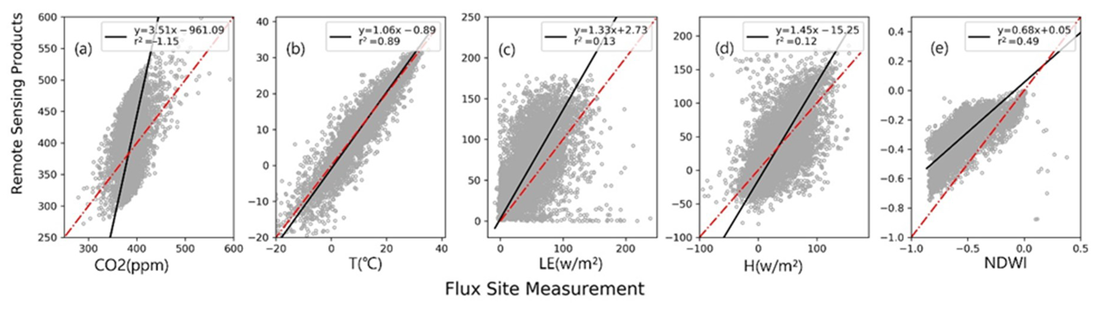
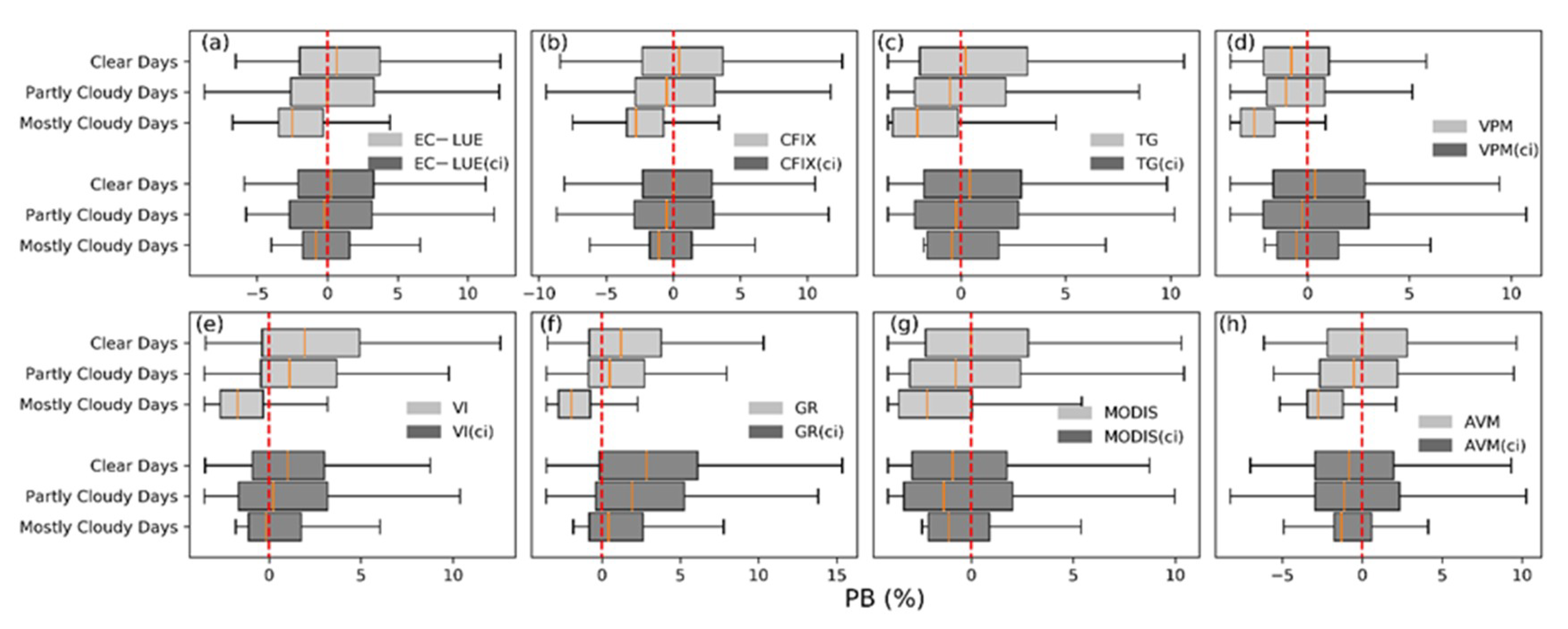
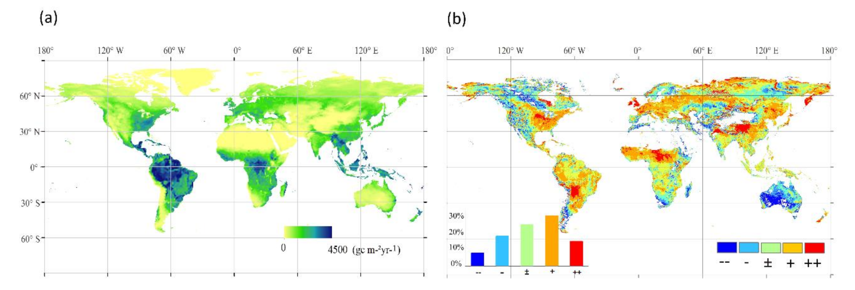
3.2. Biases in Remote Sensing Data Products and Consequences on Global GPP Estimation

First, various biases were found when the spatial datasets that feed the models for global GPP simulations were evaluated at the site scale (Figure 3 and Figure A2). For example, the spatial PAR dataset only explained 57% of the observed PAR variation at the EC-towers, and the slope and intercept were 1.2 and 0.57, respectively, indicating that the PAR data fields overestimated PAR as a whole and slightly underestimated PAR at the low value. The determination coefficients of the global datasets of CO₂, LE, and H at the EC-towers were less than 20% (R² < 0.2), and only temperature data was efficient in representing site-scale variation (R² = 0.89).

Second, the biases in the spatial datasets had a significant impact on GPP simulations was found through orthogonal regression. Before correcting these biases, the simulated GPP by the LUE-EF and LUE-NDWI models explained only 49% and 61% of the EC-tower GPP variation, and the slopes of the linear regression between simulated and tower-estimated GPP were 1.54 and 1.31, respectively, and the corresponding intercepts were −2.09 and –1.23. These results indicate that both models overestimated GPP as a whole, but underestimated low GPP values (Figure 3b,f). After correcting the biases in the spatial datasets, the R² of LUE-EF and LUE-NDWI models improved to 0.80 and 0.79, with the slopes closer to 1 (1.20 and 1.18 values, respectively) and the intercepts closer to 0 (−0.59 and −0.91, respectively) (Figure 3c,g). The results also indicated that the LUE-NDWI model was less sensitive to the biases in the spatial data fields than the LUE-EF model, as shown by the smaller differences in R² before and after data correction. This can probably be attributed to the fact that the LUE-NDWI relies on NDWI, a factor that can be derived directly from remote sensing data and thereby less prone to error propagation than the LUE-EF model.

At a global scale, the biases in spatial data inputs had a great impact on the simulated GPP even for the less sensitive model LUE-NDWI. Figure 4a shows the global average annual GPP distribution from 2000 to 2018, simulated by the LUE-NDWI model using corrected input data layers. The spatial pattern of GPP agrees well with previous studies. However, the impact of data biases on the spatial pattern of simulated GPP was obvious and not uniform across space (Figure 4b). The area overestimated is much larger than the underestimated area when the data biases were not attended, and the area fractions with GPP biases at (−50%)–(−30%), (−30%)–(−10%), 10–30%, and 30–50%, were 8%, 19%, 27%, 31%, and 15%, respectively. After data correction, the area of GPP serious reduction occurs in the mountain systems of the Tibetan plateau in Asia, northern Africa, and South America region. Growth trends of GPP were observed in Australia, northwest North America, and Siberia. The global annual average GPP estimated by the LUE-NDWI, after input data correction, was about 125.6Pg C yr⁻¹. Without data correction, the LUE-NDWI model would overestimate global GPP by 18% (Figure 5a,b). The corresponding global growth rate of GPP decreased from 0.34 to 0.17 Pg C yr⁻¹ after input data correction (Figure 5c).

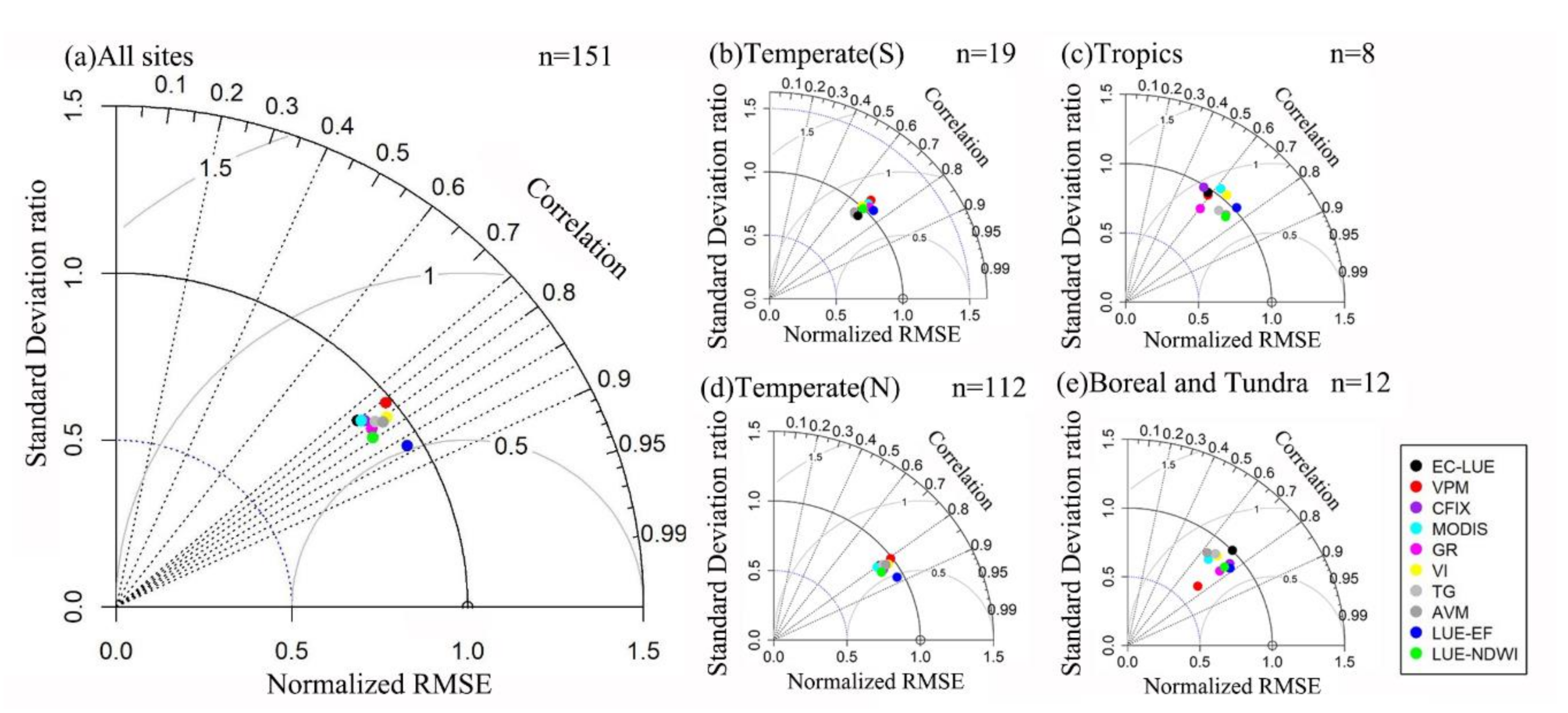
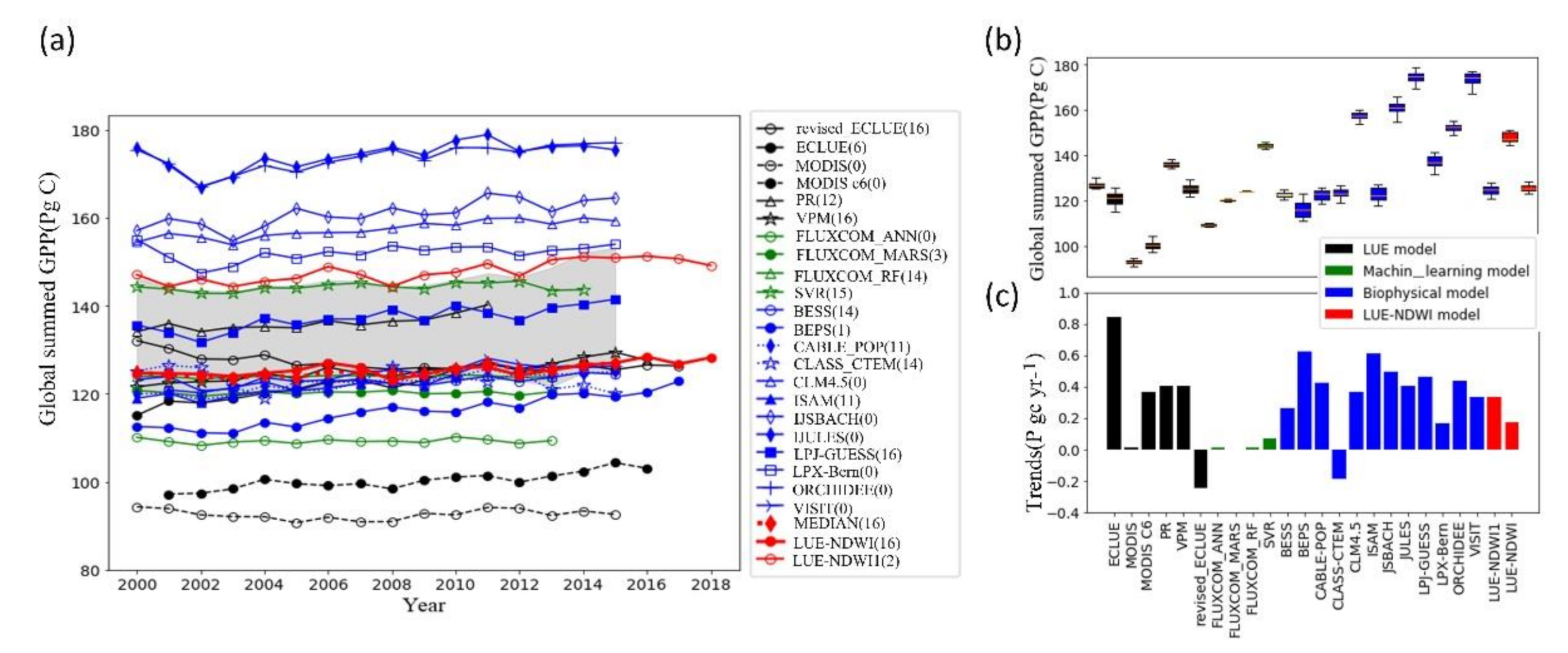
3.3. Comparison of 24 Global GPP Products

A comparison of 24 global GPP products is shown in Figure 5a. Large differences can be seen from these models with long-term GPP averages varying from 92.7 to 178.9 Pg C yr⁻¹, with more GPP estimates concentrated in the range of 120−130 Pg C yr⁻¹ (Figure 5a,b). The number of times that a model’s GPP stays within the interquartile range (IQR) of all 24 GPP products throughout the years can be used as an indicator of model performance. Result showed that the annual GPP values simulated by the following models stayed within their annual IQRs every year: Revised_ECLUE, VPM, SVR, LPJ_GUESS, and LUE-NDWI (after correcting input data biases), suggesting a better performance in simulating GPP. Although not in the category above, FLUXCOM RF, BESS, CABLE POP, and CLASS CTEM models have more than 10 years in IQR. It is worth noting that the GPP from the LUE-NDWI model, after data correction, was the closest to the median GPP value of the 24 global models.

The interannual variabilities simulated by these models were also quite different (Figure 5b). The interannual variabilities of LUE and biophysical models were generally higher than the machine learning models as shown by their standard deviation or std: ECLUE (std = 2.96 Pg C yr⁻¹), BEPS (std = 3.51 Pg C yr⁻¹), JSBACH (std = 2.97 Pg C yr⁻¹), JULES (std = 3.06 Pg C yr⁻¹), LPJ-GUESS (std = 2.66 Pg C yr⁻¹), ORCHIDEE (std = 2.91 Pg C yr⁻¹), FLUXCOM_ANN (std = 0.53 Pg C yr⁻¹), FLUXCOM_RF (std = 0.38 Pg C yr⁻¹), and FLUXCOM_MARS (std = 0.23 Pg C yr⁻¹). The standard deviation of LUE-NDWI (after correcting input data biases) model was 1.83 Pg C yr⁻¹, close to the mean standard (1.68 Pg C yr⁻¹) of all the models within the IQR range.

The trends of GPP simulated by the 24 models also varied greatly from −0.25 to 0.84 Pg C yr⁻¹ (Figure 5c). The trends of the machine learning models were smaller than those of other models. Most models showed positive trends, only the revised-ECLUE and CLASS-CTEM models showed downward trends, and some models demonstrated no significant trends (i.e., MODIS, FLUXCOM_ANN, FLUXCOM_MARS, and FLUXCOM_RF).

4. Discussion

4.1. Adequacy of Model Structure in Representing Processes

The understanding of the processes involved in GPP is fundamental to building a reliable GPP model. For example, we found that a failed incorporation of the effect of clouds on GPP in some existing models significantly underestimated GPP in areas with frequent cloudy cover (Figure A1). Under clear sky conditions, the upper canopy leaves are close to light saturation, while the lower canopy leaves are shaded and have limited light [51]. In contrast, under cloudy conditions, a higher proportion of the light in the form of diffuse radiation can reach the lower parts of the canopy, thus increasing the total photosynthetic use of PAR by vegetation [31]. Some studies indicated that a 1% increase in diffuse radiation induces a 0.94% increase in GPP [27,28]. In addition, many studies have shown that CO₂ fertilization has a significant effect on vegetation production, a dominant factor contributing to the 31% increase in global GPP since 1990 [52,53]. Nevertheless, many LUE models have not explicitly accounted for the effect of increasing atmospheric CO₂ concentration [6,31]. In our study, after incorporating the impacts of both cloud cover and CO₂, the performance of the LUE-EF and LUE-NDWI models improved compared with the original EC-LUE model: R² improved from 0.61 to 0.68 for LUE-NDWI and from 0.61 to 0.74 for LUE-EF, respectively.

Water availability is an important factor that affects GPP [13]. In this study, we adopted two alternative structural expressions to represent the impact of water stress on GPP. First, the evaporative fraction (EF) of total energy, closely related to the Bowen ratio, was used in the LUE-EF model. The relevance of LUE-EF is grounded in the fact that less energy used for ecosystem evaporation (i.e., smaller evaporative fraction) implies a stronger water limitation [33], which has largely been verified using flux tower measurements [54]. Nevertheless, the application of the LUE-EF model is hindered by the derivation of EF that required multiple steps and input data layers and is therefore prone to error propagation [55]. In order to get a direct measure of water stress and therefore minimize error propagation, from satellite observations we replaced the EF using NDWI in the LUE-NDWI model, based on the evidence that NDWI is closely related to the plant water content and thus a good proxy for plant water stress [56]. The direct use of NDWI in the LUE-NDWI model makes it ideal for mapping GPP on regional to global scales.

4.2. Input Data Biases and Possible Impacts on GPP Simulations

Evaluating the quality of input data and understanding the impact of data biases on GPP simulation are prerequisites for improving GPP simulation accuracy. In this study, we found that the data from the spatial data fields at the EC-tower sites had various systematic deviations that seriously affected GPP estimates. For example, the spatial data fields of PAR explained only 57% of the PAR variation observed at the EC-tower sites. Reasons for the data biases are mainly rooted in the influence of sensor errors and atmospheric factors (e.g., cloud and snow) [50,57,58]. In addition, attempts unifying data from different spatial and temporal resolutions also bring biases as we found that data at different resolutions sometimes had poor correlations. The reason for the existence of resolution mismatch (i.e., spatial product data pixels cannot be unified in temporal or spatial scale) is mainly caused by mixed pixels and/or different time scales (e.g., daily, eight-day, or monthly data), compared to the spatio-temporal resolution that applies to ground conditions [51,59]. In general, spatial data biases are an important cause of the uncertainty of GPP simulation, which is an important reason for the large differences in GPP estimated among existing GPP models [60,61].

A comparison of existing global GPP products shows a huge variation from 92.7 to 178.9 Pg C yr⁻¹, which is not only affected by input data biases, but also by the model structure [13,62]. One should realize that input data biases affect the model outputs differently, depending on the model structure. In our study, it was found that the LUE-EF model is more susceptible to data errors, while the LUE-NDWI model is less affected by data biases (Figure 3d). The sensitivities of the GPP models to data deviations should be systematically investigated in future research as the sensitivities have not been effectively evaluated and compared.

4.3. Improving GPP Simulation Capability: The Ways Forward

A reduction in model complexity and error accumulation should be a major consideration in improving GPP estimation. For example, the evaporative fraction parameter of the LUE-EF model involves more steps than the direct use of NDWI from satellite in the LUE-NDWI model, and consequently the risk of the error accumulation increases. The direct observation and continuous recording of NDWI as a remote sensing product is one of the main advantages of the LUE-NDWI model, which minimizes the risk of error propagation of the LUE-NDWI model at a regional to global scale. Therefore, the LUE-NDWI model is more practical and attractive in spatially-explicit simulations of GPP. In summary, the simple forms of GPP models and widely and readily available inputs, as compared with more complex global models, make them more practical for applications over large areas and better suited for attribution and uncertainty analysis [53,63].

Vastly different GPP products, as shown by the means, trends, and interannual variabilities of GPP, generated by the 24 models suggest our current ability in simulating global GPP is not encouraging (Figure 5a). For nearly 40 years of commitment to the global simulation of GPP, there does not seem to have a clear direction of improvement in GPP estimation as shown by the vast differences among GPP models in simulating global GPP. GPP model development is not explicitly directed, despite the constant emergence of new models. Our research indicates that both the structures of the models and input data are error prone. Therefore, it is necessary to optimize model structures as well as sufficient validation and calibration of the input data to improve GPP simulation.

5. Conclusions

In this study, we first developed two new GPP models, driven by convenient remote sensing data and climate variables, with an emphasis on the representations of GPP responses to cloud, CO₂, and water stress. Then, the performances of the new models along with other commonly used GPP models were appraised using GPP estimates from global eddy covariance (EC) flux towers. The quality of major spatial data layers that drive the models at the global scale was also evaluated at the EC-towers.

Two new models (LUE-EF and LUE-NDWI) showed advantages in simulating daily GPP for most biomes. Meanwhile, they had a stronger ability in capturing the spatial and temporal changes of GPP and the improvements of the new models were more apparent for tropical and northern temperate zones. Then, a new global GPP product was generated using the LUE-NDWI model. The LUE-EF model was not applied on a global scale because of the difficulty in estimating the water stress in the LUE-EF model (i.e., the evaporative fraction of net solar radiation), which cannot be readily derived from satellite observations.

Various biases were found in the spatial datasets that feed the models, affecting the simulation of GPP from site to global scales. Addressing these biases is a high priority for earth system science. In addition, large differences were found from 24 global models with long-term GPP averages varying from 92.7 to 178.9 Pg C yr⁻¹. The newly developed LUE-NDWI model (after correcting input data biases) produced a global mean annual GPP that is very close to the mean level of all the models within the inter-quantile range of GPP from all 24 models. Moving forward, a reduction in model complexity and error accumulation, validation, and calibration of the input data fields are key processes of improving GPP simulation.

The newly developed new remote sensing-based GPP model had excellent performance and could be used to estimate GPP across a range of scales. Improving the quality of input data fields should be a major research component in reducing the uncertainty in GPP simulations on regional to global scales. The existent biases of spatial data not only affect GPP simulation but more importantly hinder the simulation and understanding of the earth system. Effective correction of spatial data is critical for reducing the uncertainty in GPP simulations and research on improving data quality should be encouraged. In this regard, our research cautions using currently available spatial data for relevant research.

References

1. Campbell, J.E.; Berry, J.A.; Seibt, U.; Smith, S.J.; Montzka, S.A.; Launois, T.; Belviso, S.; Bopp, T.L.S.B.L.; Laine, M. Large historical growth in global terrestrial gross primary production. Nature 2017, 544, 84–87. [Google Scholar] [CrossRef]
2. Schaefer, K.; Schwalm, C.R.; Williams, C.; Arain, M.A.; Barr, A.; Chen, J.M.; Davis, K.J.; Dimitrov, D.; Hilton, T.W.; Hollinger, D.Y.; et al. A model-Data comparison of gross primary productivity: Results from the North American Carbon Program site synthesis. J. Geophys. Res. Space Phys. 2012, 117, 1–15. [Google Scholar] [CrossRef] [Green Version]
3. Yi Zheng, Y.; Shen, R.; Wang, Y.; Li, X.; Liu, S.; Liang, S.; Chen, J.M.; Ju, W.; Hang, L.; Yuan, W. Improved estimate of global gross primary production for reproducing its long-Term variation, 1982–2017. Earth Syst. Sci. Data Discuss. 2019, 12, 2725–2746. [Google Scholar] [CrossRef]
4. Beer, C.; Reichstein, M.; Tomelleri, E.; Ciais, P.; Jung, M.; Carvalhais, N.; Rödenbeck, C.; Arain, M.A.; Baldocchi, D.; Bonan, G.B.; et al. Terrestrial gross carbon dioxide uptake: Global distribution and covariation with climate. Science 2010, 329, 834–838. [Google Scholar] [CrossRef] [PubMed] [Green Version]
5. Xiao, J.; Chevallier, F.; Gomez, C.; Guanter, L.; Hicke, J.A.; Huete, A.R.; Ichii, K.; Ni, W.; Pang, Y.; Rahman, A.F. Remote sensing of the terrestrial carbon cycle: A review of advances over 50 years. Remote Sens. Environ. 2019, 233, 111383. [Google Scholar] [CrossRef]
6. Wang, H.; Prentice, I.C.; Keenan, T.F.; Davis, T.W.; Wright, I.J.; Cornwell, W.K.; Evans, B.J.; Peng, C. Towards a universal model for carbon dioxide uptake by plants. Nat. Plants 2017, 3, 734–741. [Google Scholar] [CrossRef] [Green Version]
7. Yuan, W.; Cai, W.; Xia, J.; Chen, J.; Liu, S.; Dong, W.; Merbold, L.; Law, B.; Arain, A.; Beringer, J.; et al. Global comparison of light use efficiency models for simulating terrestrial vegetation gross primary production based on the LaThuile database. Agric. For. Meteorol. 2014, 192–193, 108–120. [Google Scholar] [CrossRef]
8. Wagle, P.; Gowda, P.H.; Xiao, X.; Anup, K.C. Parameterizing ecosystem light use efficiency and water use efficiency to estimate maize gross primary production and evapotranspiration using MODIS EVI. Agric. For. Meteorol. 2016, 222, 87–97. [Google Scholar] [CrossRef] [Green Version]
9. Xiao, X.; Hollinger, D.; Aber, J.; Goltz, M.; Davidson, E.A.; Zhang, Q.; Moore, B. Satellite-Based modeling of gross primary production in an evergreen needleleaf forest. Remote Sens. Environ. 2004, 89, 519–534. [Google Scholar] [CrossRef]
10. Yuan, W.; Liu, S.; Zhou, G.; Zhou, G.; Tieszen, L.L.; Baldocchi, D.; Bernhofer, C.; Gholz, H.; Goldstein, A.H.; Goulden, M.L.; et al. Deriving a light use efficiency model from eddy covariance flux data for predicting daily gross primary production across biomes. Agric. For. Meteorol. 2007, 143, 189–207. [Google Scholar] [CrossRef] [Green Version]
11. Xiao, Z.; Liang, S.; Wang, J.; Xiang, Y.; Zhao, X.; Song, J. Long-Time-Series global land surface satellite leaf area index product derived from MODIS and AVHRR Surface Reflectance. IEEE Trans. Geosci. Remote Sens. 2016, 54, 5301–5318. [Google Scholar] [CrossRef]
12. Xiao, X.; Zhang, Q.; Braswell, B.; Urbanski, S.; Boles, S.; Wofsy, S.; Moore, B.; Ojima, D. Modeling gross primary production of temperate deciduous broadleaf forest using satellite images and climate data. Remote Sens. Environ. 2004, 91, 256–270. [Google Scholar] [CrossRef]
13. Zheng, Y.; Zhang, L.; Xiao, J.; Yuan, W.; Yan, M.; Li, T.; Zhang, Z. Sources of uncertainty in gross primary productivity simulated by light use efficiency models: Model structure, parameters, input data, and spatial resolution. Agric. For. Meteorol. 2018, 263, 242–257. [Google Scholar] [CrossRef]
14. Yuan, W.; Chen, Y.; Xia, J.; Dong, W.; Magliulo, V.; Moors, E.; Olesen, J.E.; Zhang, H. Estimating crop yield using a satellite-Based light use efficiency model. Ecol. Indic. 2016, 60, 702–709. [Google Scholar] [CrossRef] [Green Version]
15. Xie, X.; Li, A.; Tan, J.; Jin, H.; Nan, X.; Zhang, Z.; Bian, J.; Lei, G. Assessments of gross primary productivity estimations with satellite data-Driven models using eddy covariance observation sites over the northern hemisphere. Agric. For. Meteorol. 2020, 280, 107771. [Google Scholar] [CrossRef]
16. Yuan, W.; Cai, W.; Nguy-Robertson, A.L.; Fang, H.; Suyker, A.E.; Chen, Y.; Dong, W.; Liu, S.; Zhang, H. Uncertainty in simulating gross primary production of cropland ecosystem from satellite-Based models. Agric. For. Meteorol. 2015, 207, 48–57. [Google Scholar] [CrossRef] [Green Version]
17. Wang, H.; Jia, G.; Fu, C.; Feng, J.; Zhao, T.; Ma, Z. Deriving maximal light use efficiency from coordinated flux measurements and satellite data for regional gross primary production modeling. Remote Sens. Environ. 2010, 114, 2248–2258. [Google Scholar] [CrossRef]
18. Xiao, J.; Davis, K.J.; Urban, N.M.; Keller, K.; Saliendra, N.Z. Upscaling carbon fluxes from towers to the regional scale: Influence of parameter variability and land cover representation on regional flux estimates. J. Geophys. Res. 2011, 116, 1–15. [Google Scholar] [CrossRef] [Green Version]
19. Badgley, G.; Anderegg, L.D.L.; Berry, J.A.; Field, C.B. Terrestrial gross primary production: Using NIRV to scale from site to globe. Glob. Chang. Biol. 2019, 25, 3731–3740. [Google Scholar] [CrossRef]
20. Majasalmi, T.; Stenberg, P.; Rautiainen, M. Comparison of ground and satellite-Based methods for estimating stand-Level fPAR in a boreal forest. Agric. For. Meteorol. 2017, 232, 422–432. [Google Scholar] [CrossRef]
21. Sasai, T.; Okamoto, K.; Hiyama, T.; Yamaguchi, Y. Comparing terrestrial carbon fluxes from the scale of a flux tower to the global scale. Ecol. Model. 2007, 208, 135–144. [Google Scholar] [CrossRef]
22. Gomis-cebolla, J.; Jimenez, J.C.; Sobrino, J.A. Remote Sensing of Environment LST retrieval algorithm adapted to the Amazon evergreen forests using MODIS data. Remote Sens. Environ. 2017, 204, 401–411. [Google Scholar] [CrossRef]
23. Foga, S.; Scaramuzza, P.L.; Guo, S.; Zhu, Z.; Dilley, R.D.; Beckmann, T.; Schmidt, G.L.; Dwyer, J.L.; Hughes, M.J.; Laue, B. Cloud detection algorithm comparison and validation for operational Landsat data products. Remote Sens. Environ. 2017, 194, 379–390. [Google Scholar] [CrossRef] [Green Version]
24. Stillinger, T.; Roberts, D.A.; Collar, N.M.; Dozier, J. Cloud masking for Landsat 8 and MODIS Terra over snow covered terrain: Error analysis and spectral similarity between snow and cloud. Water Resour. Res. 2019, 55, 6169–6184. [Google Scholar] [CrossRef] [PubMed] [Green Version]
25. Wu, C.; Chen, J.M.; Desai, A.R.; Hollinger, D.Y.; Arain, M.A.; Margolis, H.A.; Gough, C.; Staebler, R.M. Remote sensing of canopy light use efficiency in temperate and boreal forests of North America using MODIS imagery. Remote Sens. Environ. 2012, 118, 60–72. [Google Scholar] [CrossRef]
26. Sims, D.A.; Rahman, A.F.; Cordova, V.D.; El-Masri, B.Z.; Baldocchi, D.D.; Bolstad, P.V.; Flanagan, L.B.; Goldstein, A.H.; Hollinger, D.Y.; Misson, L.; et al. A new model of gross primary productivity for North American ecosystems based solely on the enhanced vegetation index and land surface temperature from MODIS. Remote Sens. Environ. 2008, 112, 1633–1646. [Google Scholar] [CrossRef]
27. Veroustraete, F.; Sabbe, H.; Eerens, H. Estimation of carbon mass fluxes over Europe using the C-Fix model and Euroflux data. Remote Sens. Environ. 2002, 83, 376–399. [Google Scholar] [CrossRef]
28. Gitelson, A.A.; Viña, A.; Verma, S.B.; Rundquist, D.; Arkebauer, T.J.; Keydan, G.; Leavitt, B.; Ciganda, V.; Burba, G.G.; Suyker, A.E. Relationship between gross primary production and chlorophyll content in crops: Implications for the synoptic monitoring of vegetation productivity. J. Geophys. Res. 2006, 111, 1–13. [Google Scholar] [CrossRef] [Green Version]
29. Liu, Z.; Wang, L.; Wang, S. Comparison of different GPP models in China using MODIS image and ChinaFLUX data. Remote Sens. Sens. 2014, 6, 10215–10231. [Google Scholar] [CrossRef] [Green Version]
30. Running, S.T.; Nemani, R.R.; Heinsch, F.A.; Zhao, M.; Reeves, M. A Continuous Satellite-Derived Measure of Global Terrestrial Primary Production. Bioscience 2006, 54, 547–560. [Google Scholar] [CrossRef]
31. Wu, C.; Munger, J.W.; Niu, Z.; Kuang, D. Comparison of multiple models for estimating gross primary production using MODIS and eddy covariance data in Harvard Forest. Remote Sens. Environ. 2010, 114, 2925–2939. [Google Scholar] [CrossRef]
32. Gu, L.; Baldocchi, D.D.; Wofsy, S.C.; Munger, J.W.; Michalsky, J.J.; Urbanski, S.P.; Boden, T.A. Response of a Deciduous Forest to the Mount Pinatubo Eruption: Enhanced Photosynthesis. Science 2003, 299, 2035–2038. [Google Scholar] [CrossRef] [PubMed] [Green Version]
33. Kicklighter, D.W. A first-Order analysis of the potential rôle of CO2 fertilization to affect the global carbon budget: A comparison of four terrestrial biosphere models. Tellus B: Chem. Phys. Meteorol. 1999, 51, 343–366. [Google Scholar] [CrossRef] [Green Version]
34. Raich, J.W.; Rastetter, E.B.; Melillo, J.M.; Kicklighter, D.W.; Steudler, P.A.; Peterson, B.J.; Grace, A.L.; Moore, B.; Vorosmarty, C.J. Potential Net Primary Productivity in South America: Application of a Global Model. Ecol. Appl. 2013, 1, 399–429. [Google Scholar] [CrossRef] [PubMed] [Green Version]
35. Murphy, R.J.; Whelan, B.; Chlingaryan, A.; Sukkarieh, S. Quantifying leaf scale variations in water absorption in lettuce from hyperspectral imagery: A laboratory study with implications for measuring leaf water content in the context of precision agriculture. Precis. Agric. 2018, 767–787. [Google Scholar] [CrossRef]
36. Ding, C.; Liu, X.; Huang, F.; Li, Y.; Zou, X. Onset of drying and dormancy in relation to water dynamics of semi-arid grasslands from MODIS NDWI. Agric. For. Meteorol. 2017, 234–235, 22–30. [Google Scholar] [CrossRef]
37. Pastorello, G.; Trotta, C.; Canfora, E.; Chu, H.; Christianson, D.; Frank, J.; Frank, J.; Massman, M.; Urbanski, S. The FLUXNET2015 dataset and the ONEFlux processing pipeline for eddy covariance data. Sci. Data 2020, 7, 225. [Google Scholar] [CrossRef]
38. Baty, F.; Ritz, C.; Charles, S.; Brutsche, M. A toolbox for nonlinear regression in R: The package nls tools. J. Stat. Softw. 2015, 66, 1–21. [Google Scholar] [CrossRef] [Green Version]
39. Zhang, F.; Shi, X.; Zeng, C.; Wang, L.; Xiao, X.; Wang, G.; Chen, Y.; Zhang, H.; Lu, X.; Immerzeel, W. Recent stepwise sediment flux increase with climate change in the Tuotuo River in the central Tibetan Plateau. Sci. Bull. 2020, 65, 410–418. [Google Scholar] [CrossRef] [Green Version]
40. Carroll, R.J.; Ruppert, D. The Use and Misuse of Orthogonal Regression in Linear Errors-in-Variables Models. General 2014, 50, 1–6. [Google Scholar]
41. Piñeiro, G.; Perelman, S.; Guerschman, J.P.; Paruelo, J.M. How to evaluate models: Observed vs. predicted or predicted vs. observed? Ecol. Model. 2008, 216, 316–322. [Google Scholar] [CrossRef]
42. Leng, L.; Zhang, T.; Kleinman, L.; Zhu, W. Ordinary least square regression, orthogonal regression, geometric mean regression and their applications in aerosol science. J. Phys. Conf. Ser. 2007, 78, 24–28. [Google Scholar] [CrossRef]
43. Valbuena, R.; Hernando, A.; Manzanera, J.; Görgens, E.; Almeida, D.; Mauro, F.; García-Abril, A.; Coomes, D. Enhancing of accuracy assessment for forest above-Ground biomass estimates obtained from remote sensing via hypothesis testing and overfitting evaluation. Ecol. Model. 2017, 366, 15–26. [Google Scholar] [CrossRef] [Green Version]
44. Forzieri, G. Increased control of vegetation on global terrestrial energy fluxes. Nat. Clim. Chang. 2020, 10, 356–362. [Google Scholar] [CrossRef]
45. Running, S.W.; Zhao, M. Daily GPP and Annual NPP (MOD17A2/A3) products NASA Earth Observing System MODIS Land Algorithm-User’s guide V3. General 2015, 28, 1–6. [Google Scholar]
46. Keenan, T.F.; Prentice, I.C.; Canadell, J.G.; Williams, A.C.; Wang, H.; Raupach, M.; Collatz, G.J. Recent pause in the growth rate of atmospheric CO2 due to enhanced terrestrial carbon uptake. Nat. Commun. 2016, 7, 1–9. [Google Scholar] [CrossRef] [Green Version]
47. Jung, M.; Schwalm, C.; Migliavacca, M.; Walther, S.; Camps-Valls, G.; Koirala, S.; Anthoni, P.; Besnard, S.; Bodesheim, P.; Carvalhais, N.; et al. Scaling carbon fluxes from eddy covariance sites to globe: Synthesis and evaluation of the FLUXCOM approach. Biogeosciences 2020, 17, 1343–1365. [Google Scholar] [CrossRef] [Green Version]
48. Kondo, M.; Ichii, K.; Takagi, H.; Sasakawa, M. Comparison of the data-Driven top-Down and bottom-Up global terrestrial CO2 exchanges: GOSAT CO2 inversion and empirical eddy flux upscaling. J. Geophys. Res. Biogeosci. 2015, 120, 1226–1245. [Google Scholar] [CrossRef]
49. Jiang, C.; Ryu, Y. Remote Sensing of Environment Multi-Scale evaluation of global gross primary productivity and evapotranspiration products derived from Breathing Earth System Simulator (BESS). Remote Sens. Environ. 2016, 186, 528–547. [Google Scholar] [CrossRef]
50. Upadhyaya, S.A.; Kirstetter, P.-E.; Gourley, J.J.; Kuligowski, R.J. On the Propagation of Satellite Precipitation Estimation Errors: From Passive Microwave to Infrared Estimates. Estimates. J. Hydrometeorol. 2020, 21, 1367–1381. [Google Scholar] [CrossRef]
51. Cheng, S.J.; Butterfield, Z.; Keppel-Aleks, G.; Steiner, A.L. The Global Influence of Cloud Optical Thickness on Terrestrial Carbon Uptake. Earth Interact. 2019, 23, 1–22. [Google Scholar]
52. Haverd, V.; Smith, B.; Canadell, J.G.; Cuntz, M.; Mikaloff-Fletcher, S.; Farquhar, G.D.; Woodgate, W.; Briggs, P.R.; Trudinger, C.M. Higher than expected CO 2 fertilization inferred from leaf to global observations. Glob. Chang. Biol. 2020, 26, 2390–2402. [Google Scholar] [CrossRef] [PubMed] [Green Version]
53. Smith, W.K.; Reed, S.C.; Cleveland, C.C.; Ballantyne, A.P.; Anderegg, W.R.L.; Wieder, W.R.; Liu, Y.Y.; Running, S.W. Large divergence of satellite and Earth system model estimates of global terrestrial CO2 fertilization. Nat. Clim. Chang. 2016, 6, 306–310. [Google Scholar] [CrossRef]
54. Chen, Y.; Xia, J.; Liang, S.; Feng, J.; Fisher, J.B.; Li, X.; Li, X.; Liu, S.; Ma, Z.; Miyata, A.; et al. Comparison of satellite-based evapotranspiration models over terrestrial ecosystems in China. Remote Sens. Environ. 2014, 140, 279–293. [Google Scholar] [CrossRef]
55. Ma, H.Y. CAUSES: On the Role of Surface Energy Budget Errors to the Warm Surface Air Temperature Error Over the Central United States. J. Geophys. Res. Atmos. 2018, 123, 2888–2909. [Google Scholar] [CrossRef] [Green Version]
56. Gao, B.-C. NDWI—A normalized difference Water index for remote sensing of vegetation liquid water from space. Remote Sens. Environ. 1996, 266, 257–266. [Google Scholar] [CrossRef]
57. Keppel-Aleks, G.; Washenfelder, R.A. The effect of atmospheric sulfate reductions on diffuse radiation and photosynthesis in the United States during 1995–2013. Geophys. Res. Lett. 2016, 43, 9984–9993. [Google Scholar] [CrossRef]
58. Lee, M.S.; Hollinger, D.Y.; Keenan, T.F.; Ouimette, A.P. Agricultural and Forest Meteorology Model-based analysis of the impact of di ff use radiation on CO 2 exchange in a temperate deciduous forest. Agric. For. Meteorol. 2018, 249, 377–389. [Google Scholar] [CrossRef] [Green Version]
59. Sun, Z.; Wang, X.; Zhang, X.; Tani, H.; Engliang, G.; Shuai, Y.; Zhang, T. Science of the Total Environment Evaluating and comparing remote sensing terrestrial GPP models for their response to climate variability and CO2 trends. Sci. Total Environ. 2019, 668, 696–713. [Google Scholar] [CrossRef]
60. Xie, X.; Li, A. Development of a topographic-Corrected temperature and greenness model (TG) for improving GPP estimation over mountainous areas. Agric. For. Meteorol. 2020, 295, 108193. [Google Scholar] [CrossRef]
61. Zhang, Z.; Zhang, Y.; Zhang, Y.; Chen, J.M. Correcting Clear-Sky Bias in Gross Primary Production Modeling From Satellite Solar-Induced Chlorophyll Fluorescence Data. J. Geophys. Res. Biogeosci. 2020, 125, e2020JG005822. [Google Scholar] [CrossRef]
62. Flack-Prain, S.; Meir, P.; Malhi, Y.; Smallman, T.; Williams, M. The importance of physiological, structural and trait responses to drought stress in driving spatial and temporal variation in GPP across Amazon forests. Biogeosciences 2019, 16, 4463–4484. [Google Scholar] [CrossRef] [Green Version]
63. Ren, Y.; Zhang, F.; Kung, H.-T.; Johnson, V.C.; Wang, J.; Zhang, Y.; Yu, H.; Yushanjiang, A. Using the vegetation-solar radiation (VSr) model to estimate the short-term gross primary production (GPP) of vegetation in Jinghe county, XinJiang, China. Ecol. Eng. 2017, 107, 208–215. [Google Scholar] [CrossRef]
Figure 1. The Taylor diagram showing (a) the performance of all models, data from eddy covariance (EC) towers were used.; (be) the performance of all models in different latitudinal geographical zones (tropics:−23.5° –23.5°, temperate:−23.5° −(−66.5°) and (23.5°−66.5°), boreal and tundra: 66.5°–90°), where N and S represent the Northern and Southern hemispheres, respectively. The upper right corner of subplot "n" is number of EC-towers.
Remotesensing 13 00168 g001
Figure 2. Comparison of cumulative gross primary production (GPP) estimates from the flux towers and the models. The color lines represent the GPP value of cumulative comparison between the EC-tower and model for each site. The red dashed line is the 1:1 reference to the differences of modeled GPP and EC-tower. Inset histogram shows the frequency distribution of the percentage biases (PB) at the flux towers. The two shaded plots (panels i and j) are two new models devel-oped in this study. (a) EC-LUE (eddy covariance-light use efficiency model), (b) VPM (vegetation photosynthesis model), (c) CFIX (carbon fixation model), (d) MODIS (moderate resolution imaging spectroradiometer model), (e) GR (green-ness-radiation model), (f) VI (vegetation-indices model), (g) TG (temperature-greenness model), (h) AVM (alpine vegetation model), (i) LUE-EF (light use efficiency-evaporative fraction model), (j) LUE-NDWI (light use efficiency-normalized difference water index model).
Remotesensing 13 00168 g002
Figure 3. Comparison of (a) spatial PAR (photosynthetic active radiation) and site PAR, (b) tower GPP and LUE-EF GPP (uncorrected spatial data), (c) tower GPP and LUE-EF GPP (corrected spatial data), (d) LUE-EF GPP with uncorrected and LUE-EF GPP corrected spatial data, (e) spatial EVI (500 m resolution) and spatial EVI (10 km resolution), (f) tower GPP and LUE-NDWI GPP (uncorrected spatial data), (g) tower GPP and LUE-NDWI GPP (corrected spatial data), and (h) LUE-NDWI GPP with uncorrected and LUE-NDWI GPP corrected spatial data. All comparisons are based on site scale. Corrected spatial data were generated from the uncorrected ones after correcting their biases using orthogonality regression (see Section 2.5).
Remotesensing 13 00168 g003
Figure 4. Consequences of biased input data on LUE-NDWI GPP at a global scale. (a) The mean annual GPP from 2000 to 2018 after data correction (reference Section 2.5). (b) The difference of mean annual GPP from 2000 to 2018, GPPuncorrected—GPPcorrected. Symbols indicate various levels of difference: ‘--’: −50%–(−30%), ‘-’: −30%–(−10%), ‘±’: −10%–10%, ‘+’: 10–30%, ‘++’: 30–50%. The inset bar chart shows the global distribution of the difference proportions.
Remotesensing 13 00168 g004
Figure 5. (a) Comparison of annual global GPP estimates from various models. The number after each model’s name in parentheses is the model’s number of years in the interquartile range (IQR) of all global GPP products, indicated by the shaded region. LUE-NDWI (data corrected) and LUE-NDWI1(i.e., LUE-NDWI with spatial data uncorrected) are GPP estimated by LUE-NDWI with corrected and uncorrected input data, respectively. (b) Boxplot of annual GPP values during the study period for each model. (c) Trends of annual GPP (Pg C yr−1) by model. Symbols of LUE models are in black, machine learning models in green, and biophysical models in blue.
Remotesensing 13 00168 g005
Publisher’s Note: MDPI stays neutral with regard to jurisdictional claims in published maps and institutional affiliations.