Predicting Future Urban Flood Risk Using Land Change and Hydraulic Modeling in a River Watershed in the Central Province of Vietnam

Abstract

Flood risk is a significant challenge for sustainable spatial planning, particularly concerning climate change and urbanization. Phrasing suitable land planning strategies requires assessing future flood risk and predicting the impact of urban sprawl. This study aims to develop an innovative approach combining land use change and hydraulic models to explore future urban flood risk, aiming to reduce it under different vulnerability and exposure scenarios. SPOT-3 and Sentinel-2 images were processed and classified to create land cover maps for 1995 and 2019, and these were used to predict the 2040 land cover using the Land Change Modeler Module of Terrset. Flood risk was computed by combining hazard, exposure, and vulnerability using hydrodynamic modeling and the Analytic Hierarchy Process method. We have compared flood risk in 1995, 2019, and 2040. Although flood risk increases with urbanization, population density, and the number of hospitals in the flood plain, especially in the coastal region, the area exposed to high and very high risks decreases due to a reduction in poverty rate. This study can provide a theoretical framework supporting climate change related to risk assessment in other metropolitan regions. Methodologically, it underlines the importance of using satellite imagery and the continuity of data in the planning-related decision-making process.

1. Introduction

Floods are a frequent and damaging natural disaster that negatively impacts the socioeconomic development and lives of millions of people worldwide [1,2,3,4,5]. It is estimated that between 1990 and 2016, worldwide losses from flood damage amounted to USD 723 billion [6]. Due to population growth and climate change, urban areas in particular are expected to be seriously threatened by the effects of increased flood intensity and frequency [7,8,9,10]. Approximately 40% of the world’s cities will be in areas under high flood risk by 2030, thereby affecting about 54 million people [11]. Furthermore, 82% of urban areas in Southeastern Asia will be in high-frequency flood zones by 2030 [12]. Understanding the complex relationships between urban growth and floods is essential in developing risk management strategies for sustainable land use planning [13].

The flood system is very complicated and has the characteristics of spatial-temporal dynamics, with uncertainties and integration of different challenges in a system generating complex phenomena [14]. Research is an essential tool in flood risk management since it plays an essential role in predicting flood hazard and improving societal comprehension of the complex environmental and socioeconomic components of flood risk [15]. The objective of this study is to develop a comprehensive approach to estimating the evolution in flood risk between 1995 and 2040 in a rapidly changing land cover context in Vietnam.

Flood risk is a combination of hazard, exposure, and vulnerability [16], so risk can be managed by reducing the flood intensity and/or damage [17,18]. Over the past few decades, with the development of science, the world has brought many changes in the approach to minimize flood effects. Traditional methods of flood control (i.e., structural measures such as dikes, embankments, etc.) are gradually being replaced by more comprehensive flood risk management models [19,20]. These approaches take into account the probabilities and potential consequences of flood events based on risk assessment studies where flood hazard and exposure/vulnerability factors are quantified [21]. Several methods have been applied to compute these indicators. The hazard approaches include: measurement-based, field surveys [22,23], hydrodynamic models [24,25], and GIS and Remote Sensing [26,27] in linear modeling of flood risk through overlaying component layers with associated analytical hierarchical process (AHP)-based computed weights. Land cover indicators can be grouped into two categories: (1) traditional terrestrial mapping [28]; and (2) land cover classification based mainly on satellite observations [29,30]. The emergence of satellite sensors like Landsat, Satellite Pour Observation de la Terre (SPOT), and Sentinel 2, among others, has greatly facilitated the rapid classification of land cover and its evolution. In addition, remote sensing has the advantage of rapid data acquisition with lower costs over field survey methods [31].

Flood risk assessment is an essential step in defining appropriate management strategies [32]. In recent decades, several studies have focused on developing flood risk assessment methods at different scales and with different objectives. Mishra et al. [33] developed a flood risk index for the Kosi River of India based on hazard (geomorphologic, distance to the active channel, slope, and rainfall) and socioeconomic vulnerability (population, household, and female densities; literacy rates; land cover and use changes; road–river intersections; road density). Chinh Luu et al. [34] studied the temporal changes of flood risk that integrated hazard, exposure, and vulnerability to better understand the evolving dynamics and formulate appropriate mitigation strategies. Dang et al. [35] outlined the essential roles in improving flood risk assessment methods to support decision-making processes. The authors classified flood risk indices into three components: social–economic, physical, and environmental. Kron [36] constructed flood risk indices based on the likelihood of flood occurrence, social–economic vulnerability, the environment, and flood consequences. Begun et al. [37] integrated floods-related damage with the probability of their occurrence. Several clues or methods of assessing flood risk have been developed in different areas. However, they are limited in a comprehensive framework that can support decision-makers to understand the aggravating risk causes. In addition, these studies focus on assessing the flood risk at a specific time while, according to Penning-Rowell et al. [38], flood risk reduction strategies are most effective when they are evaluated continuously. Jhong et al. [39] emphasize that understanding hazard, exposure, and vulnerability at different dates is an essential task in flood risk reduction that allows land managers to better see the spatial and temporal trends likely to arise in the future [40]. To fill the gaps identified, we integrate hydraulic modeling with land cover change analysis and prediction to assess flood risk at three dates: 1995, 2019, and 2040.

This research is different from the previous studies cited because it provides a novel and comprehensive approach to flood risk assessment based on state-of-the-art remote sensing and modeling techniques and assesses both historical and future trends. The initial hypothesis tested in this study is that flooding risk has increased substantially in the study area due to an increase in the population living in the flood plain. Flood hazard, exposure, and vulnerability were all accounted for in order to assess their potential interactions and compensatory effects. While this study explicitly examines flood risk in a catchment located in Vietnam, the findings are of importance to other rapidly evolving countries affected by floods and experiencing urban growth.

2. Study Area Characteristics

With an area of 5152.67 km², Quang Ngai province is located in Vietnam’s central coastal region (Figure 1). In 2019, the total population was approximately 1.23 million, with a density of 237 people per km². The Tra Khuc River watershed within the city of Quang Ngai is central to the economy of the province; therefore, urbanization is growing rapidly. The population has increased from 1,218,600 in 2010 to 1,231,697 in 2019, with most of this growth occurring in the alluvial plains subject to floods. Apart from Ly Son Island, the Tra Khuc River watershed covers all Quang Ngai province districts. Its topography can be divided into three main segments: upslope, downslope, and smaller alluvial plains. Upslope, the catchment is dominated by steep slopes, narrow valleys, and gorges. Downstream, an extensive plain can be found at Quang Ngai city’s location just before the channel’s outlet into the East Sea. Between the upslope and downstream zones, smaller alluvial plains lie along the main river channels between the uplands.

The two main rivers forming the watersheds are the Tra Khuc River and the Ve River. Most rivers and streams originate from the Truong Son mountain range and flow into the East Sea with a common feature being shallow, narrow riverbeds and strong seasonal variations in channel width and discharge. While the Ve River has a length of 91 km, the Tra Khuc River is one of the largest rivers in central Vietnam and is nearly 135 km long.

A tropical monsoon regime influences the climate in this region, with distinct rainy and dry seasons. The dry season runs from April to August, and the rainy season runs from September to March; it is usually characterized by intense rainfall resulting from tropical depressions and storms. The average annual rainfall ranges from 2000 to 2500 mm with 80% of it occurring between September and December and heavy typhoon rains cause floods in the Tra Khuc watershed. The November 2013 flood caused 41 deaths and resulted in the evacuation of nearly 1700 households in addition to other substantial damage and is considered one of the most significant damage-causing events in Quang Ngai province’s history. This event was selected as the case study for this research (Figure 1).

3. Data and Methods

In this study, flood risk is determined by a combination of flood hazard, exposure, and vulnerability. Hazard is a physical phenomenon—natural and uncontrollable with intense occurrence [41]. It is an elementary notion that expresses the probability of a situation, an event, or some causality—a flood in this case [36,42]. It is directly proportional to the intensity of the phenomenon’s occurrence [43], since the combination of flood depth and flood peak velocity represents the capacity to destroy objects in the area through which the flood passes, directly affecting houses, buildings, and people’s lives and health. Exposure is understood as values present at the location of a possible flood. These values can be goods, infrastructure, cultural heritage, people, or agricultural areas. This can be interpreted as the presence or availability of assets and people in flood risk areas. The level of exposure depends on the frequency of flood occurrence, the flood’s intensity, and the value of the available properties and people [42,44]. In this study, land cover and population density were selected to analyze the level of exposure. The land cover categories are detailed below and include Cropland, Forest, Urban area, and Water. Potential flood impacts in urban areas are considered greater since the infrastructure is well developed and they concentrate more value than other land cover types; they also have the greatest population densities. Agricultural land follows urban areas as it provides the livelihood for many of the watershed inhabitants. Population density is a critical variable of flood exposure analysis; because it is linked directly with humans, it is proportional with the level of flood vulnerability [34]. Vulnerability represents the lack of individuals’ or groups’ ability or capacity to anticipate, counter, and resist floods [45]. The International Plant Protection Convention (IPPC) emphasizes that these capacities depend on the prevailing economic situation and social and political characteristics. Vulnerability increases in direct proportion to the flood level and decreases socioeconomic wellbeing during floods [46]. In this study, the poverty rates and number of hospitals were selected to build the vulnerability maps. The wealthy-to-poor ratio characterizes a community’s resilience; the wealthy have sturdier homes, have the ability to access information about danger through modern media, and quick resumption of their normal lives is enhanced by their good economic standing [47]. Hospitals play a critical role during and after events. Patients place a heavy burden on communities and emergency management services in the event of an evacuation [48]. A flowchart of the methodological workflow is displayed in Figure 2. The quantification of hazards, vulnerability, and exposure is described in detail in the following sections.

3.1. Flood Hazard Estimation

Flow depth and velocity were used to estimate flood hazard. The hydraulic modeling tool MIKE FLOOD, which combines the MIKE 11 and MIKE 21 models, was used to build the depth and velocity map for the 2013 Quang Ngai historic flood.

3.1.1. Establishing the 1-Dimensional (1D) River Network

The 1D network is necessary for modeling water flow through the channels into the flood plains and was established for the Ve and Tra Khuc rivers with 46 cross-sections along 27.1 km of the Ve River (average distance about 0.59 km/sections), and 21 cross-sections along 51.6 km of the Tra Khuc (average distance about 2.6 km/sections). The cross-sections were measured directly in the field using total station (Figure 1). The discharge observation data at An Chi and Son Giang gauges were applied to the upstream boundary of Ve and Tra Khuc, respectively, and the tide level was applied to the downstream boundary using tidal sea level harmonic constants. MIKE NAM is the rainfall runoff model part of the MIKE 11 module developed by the Danish Hydraulic Institute (DHI), Denmark. This model provided discharge for sub-basins without streamflow data, and sub-catchment boundaries are presented in Figure 1. MIKE NAM was integrated into the MIKE 11 model and values were applied to the inflow boundaries for the MIKE 11 hydraulic model.

3.1.2. Establishing the River Network in the 2-Dimensional (2D) Hydraulic and FLOOD Models

The 2D channel network is necessary for estimating the spatial extent of the flooded areas when the river depth exceeds bank height. The area modeled covered an area of 507.2 km² based on the surface elevation data and observed flood inundation area defined by flood marks. The 1:10,000 topographic map published in 2010 by the Ministry of Water Resources and Environment was used for defining the 2D domain’s elevation in MIKE-21. The 2D computational mesh was generated by discretizing the computational domain into 48,200 elements, with the size of elements ranging from 457 to 2500 m².

MIKE FLOOD is used to link MIKE 11 and MIKE 21 through the Lateral link which connects the tops of riverbanks in the 1D model to the 2D model’s mesh elements. The water levels and time series of two flood events—one in November 2013 and the other in November 2017 at Tra Khuc gauge—served to calibrate and validate the model. Parameters for the 2D model were calibrated based on flood trace measurements taken in November 2013 (50 locations) and November 2017 (32 locations). Nash–Sutcliffe efficiency (NSE) [49], flood peak error, and coefficient of determination (R²) were used to measure the model’s reliability.

3.2. Indicators of Flood Exposure

Exposure was quantified based on property value and the population [22,24]; land-use categories and population density were selected to estimate these variables.

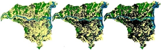
3.2.1. Land Cover Mapping in 1995, 2019, and 2040

Land Cover Mapping in 1995 and 2019

Land cover maps were created using satellite imagery—SPOT-3 (12/03/1995) with a 20 m spatial resolution and Sentinel-2 (27/02/2019) with a 10 m resolution, for 1995 and 2019, respectively. The data were projected to a common datum and coordinate system (WGS84/UTM Zone 48N). Both images were acquired with cloud cover less than 5%. Images underwent radiometric and geometric corrections before re-sampling all bands to a 10 m spatial resolution using the bilinear interpolation sampling method.

The eCognition Developer of Trimble was used to perform object-oriented classification on the SPOT-3 and Sentinel-2 images; a sample output of the classification process is displayed in Figure 3. First, image objects were segmented by integrating similar pixels; then, each segment was assigned to land cover object layers [50,51]. In order to optimize the object-oriented classification, it was necessary to select the appropriate segmentation parameters as each segment must be homogeneous and separate from its neighbors [52].

Values for the 3 segmentation parameters were 400 for Scale, 0.2 for Shape, and 0.99 for Compactness. After segmentation, the objective variables were selected using random formation points, and the information related to the objects was extracted. Different values of objective characteristics were derived from spectral indices such as the Normalized Difference Vegetation Index (NDVI) and the Enhanced Vegetation Index (EVI). The samples and extracted objective information were then exported to a calculation table. The object-oriented classification was based on the training polygons with 5 land-use categories: Cropland, Developed (built area), Bare soil, Forest, and Water bodies.

The land cover map in 1995 was compared to panchromatic aerial photographs collected from the Ministry of Natural Resources and Environment (MONRE 1995), while the 2019 classification was compared to the 2020 land use map (MONRE 2020). Validation points were randomized with n = 205 for the map in 1995 and n = 262 for the map in 2019; the number of sampling points for each class depended on the class coverage.

Change Prediction in 2040

The initial map had five categories, but Bare soil was mostly sand bars in the river or exposed beach areas along the coast, so it was integrated into the Water body category to facilitate land cover change modeling.

Future land cover change was modeled using the Land Change Modeler (LCM) module from Terrset [53] using the default Multi-Layer Perceptron (MLP) neural network option for predicting future change. LCM facilitates the quantification and mapping of historical land cover changes and predicts future changes based on past transition rates. Quantity of change from one land cover to another is based on Markov chain analysis, and spatial allocation depends on transition potentials derived from historical trends and explanatory variables such as topographic or distance variables [53,54]. Driver variables generally belong to one of three categories: accessibility, suitability, and zoning [55]. Accessibility is frequently modeled as the distance from roads or existing urban areas, and suitability for urban areas is strongly dependent on topography. There were no zoning constraints or initiatives in the study area. The initial explanatory variables tested were the following: altitude (10 m DEM), slope inclination (%), and distances from roads, developed area in 1995, and from water (river or sea). However, since slope inclination and altitude are closely correlated in the study area, only altitude was retained. The contribution of explanatory variables to predicting land cover change was estimated from Cramer’s V values and from accuracy rates produced during the creation of potential transition layers [53]. Accuracy rates are calculated by running calibrating transitions on a sub-sample of cells and then evaluating the accuracy of predictions on the remaining cells. A land cover map for 2040 was produced from the transition potential maps.

3.2.2. Population Density

Population density is considered one of the critical indices for flood exposure. Population density by municipality was obtained from the municipalities for 1995 and 2019, and an estimate for 2040 by the municipalities, was obtained from the statistics and general offices of six districts in the study area (Quang Ngai, Son Tinh, Mo Duc, Tu Nghia, Nghia Hanh, and Binh Son).

3.3. Indicators of Flood Vulnerability

Poverty data by municipality and number of hospitals in the flood zone were obtained from six Departments of Statistics (Quang Ngai, Son Tinh, Mo Duc, Tu Nghia, Nghia Hanh, Binh Son) to build the vulnerability map as described below.

3.4. Assigning Normalized Weights for Hazard, Exposure and Vulnerability Using Analytical Hierarchical Process (AHP)

The components of flood risk are hazard, exposure, and vulnerability [36,56,57]. Each component was divided into sub-components and the AHP method was used to quantify the weight of each sub-component [35].

AHP is a quantitative method used to organize decision options and choose an option that satisfies a given criterion. Developed by Thomas L. Saaty in the 1970s, it is considered an efficient and flexible method for analyzing multi-criteria decisions [58]. It operates by setting priorities for multi-criteria rankings that are judged by experts involved in the decision-making process to derive the best decision possible. In this study, assessments were based on the authors’ group experience and from previous similar studies [35,59,60,61,62,63]. The weights of flood risks in 4 steps:

(1)

Constructing component and sub-component hierarchies: hazard, exposure, and vulnerability. Hazard is divided into two sub-components (depth and velocity), exposure into two sub-components (land cover and population density), and vulnerability into two sub-components (poverty rate and number of hospitals).

(2)

Establishing priorities: The relative importance of the elements in each pair of sub-components was evaluated subjectively and assigned a value ranging from 1 to 9 as per the Saaty scale [64].

(3)

After preparing a pairwise comparison matrix (

Table 1. Comparison matrix for flood hazard, exposure, and vulnerability indicators.

Hazard	Flood Depth	Velocity
Flood depth	1	3
Velocity	1/3	1
Column total	1.33	4
Exposure	Population Density	Land Use
Population density	1	2
Land use	1/2	1
Column total	1.5	3
Vulnerability	Poverty Rates	Number of Hospitals
Poverty rates	1	2
Number of hospitals	1/2	1
Column total	1.5	3

), each column was divided by the corresponding sums to obtain the priority factors. This process is a normalized Eigenvector of the matrix (

Table 2. Normalized matrix of flood hazard, exposure, and vulnerability.

Hazard	Flood Depth	Velocity	Sum	Average
Flood depth	0.75	0.75	1.5	0.75
Velocity	0.25	0.25	0.5	0.25
Exposure	Population Density	Land use	Sum	Average
Population density	0.66	0.66	1.32	0.66
Land use	0.34	0.34	0.68	0.34
Vulnerability	Poverty Rates	Number of Hospitals	Sum	Average
Poverty rates	0.66	0.66	1.32	0.66
Number of hospitals	0.34	0.34	0.68	0.34

); the average values of the row were used as the priority of the subcomponents to calculate flood risk.

(4)

Estimation of the Consistency Ratio (CR).

The Consistency Ratio (CR) is used to ensure consistency in the experts’ judgement throughout the application and is applied as follows:

CR = CI/RI, where Consistency Index (CI) can be calculated as per the equation CI = (λmax − n)/(n − 1); λmax is the comparison matrix’s eigenvalue obtained by multiplying each parameter’s correlation matrix column’s total summation by the normalized value of corresponding parameters; and n is the number of elements compared in pairs during a calculation.

RI must be defined in [64]

After calculating the relative importance and determining the weight of each factor in the hierarchy, flood hazard, exposure, and vulnerability were calculated using the following equations:

Flood hazard = 0.75 flood depth + 0.25 velocity

Flood exposure = 0.66 population density + 0.34 land cover

Vulnerability = 0.66 poverty rates + 0.34 number of hospitals

The output values were normalized, ranging from 0 to 1, and reclassified into five classes using the natural break method: Very low, Low, Moderate, High, and Very high.

4. Results

4.1. Flood Hazard Mapping

The differences between observed and simulated water level are illustrated in Figure 4a,b. Results from recorded flood events (

Table 3. Metric for model performance evaluation.

Metric	Flood Event in November 2013	Flood Event in November 2017
NSE	0.96	0.95
Error flood peak	9 cm (1%)	3 cm (0.4%)
R2	0.95	0.96

) indicate a good match between observation and simulation; the flood peak error ranged from 3 to 9 cm (0.4–1% of peak flow depth) for both calibration and validation. The R² values were about 0.95-0.96, and the NSE value for water level ranged from 0.95 to 0.96.

Surveyed and simulated flood values are shown in Figure 5. R², the correlation coefficient between observed measurements and simulated values at these checkpoints, reaches 0.99 for calibration and validation. The model was therefore considered reliable for estimating flood hazard.

From the hydrodynamic modeling, flood depth and velocity were mapped (Figure 6a). About 69.66 km² (29.3%) of the study area flooded to a depth of less than 0.5 m, 51.48 km² (21.7%) flooded to between 0.5 and 1 m, 70.33 km² (29.7%) flooded to between 1 and 2 m, 30.37 km² (12.7%) flooded to between 2 and 3 m, and 15.74 km² (6.67%) flooded to depths greater than 3 m.

About 107.68 km² (45.3%) is affected by a velocity under 0.33 m/s, 96.51 km² (40.6%) by a velocity between 0.33 and 0.87 m/s, 22.85 km² (9.6%) by a velocity between 0.87 and 1.81 m/s, 7.64 km² (3.2%) by a velocity between 1.8 and 3.1 m/s, and 2.93 km² (1.2%) by a velocity over 3.1 m/s (Figure 6b).

As described above, the hazard map combines both depth and velocity; about 141.09 km² (59.3%) of the flood zone is located in the very low zone, 69.8 km² (29.3%) in the low zone, 11.06 km² (4.7%) in the moderate zone, 2.56 km² (1.07%) in the high zone, and 2.67 km² (1.1%) in the very high zone. The moderate, high, and very high zones are concentrated along the river in Son Tinh, Tu Nghia, and Quang Ngai city (Figure 6c).

4.2. Flood Exposure Mapping

4.2.1. Land Cover Change in 1995, 2019, and 2040

The classification accuracy for the land cover values shown in

Table 4. Land cover and land cover changes (km²) for 1995 and 2019.

Land Cover	1995	2019	Change (km2)	Change (%)
Cropland	285.8	190.5	−95.3	−33.3
Forest	103.9	101.1	−2.8	−2.7
Built-up area	96.3	189.1	92.8	96.4
Water	28.2	34.8	6.6	23.2
Bare soil	7.2	5.9	−1.3	−18.4
Total	521.5	521.5

is 78% in 1995 and 82% in 2019. In 1995, Cropland occupied more than half the landscape (54.8%) followed by Forest and Developed with similar areas at 19.9% and 18.5% of the landscape, respectively. Water and Bare soil combined account for less than 7% of the landscape. Forested areas tend to concentrate on steeper slopes at higher altitudes near the study area’s northern and western zones (Figure 7a,b). Mean slope and altitude values for Forest are 8.2% and 19.3 m, respectively. Corresponding values for Cropland are 1.3% and 7.0 m, respectively, and values for Built-up area are 1.9% and 8.5 m, respectively; therefore, topography clearly influences land cover distribution and is a suitable land cover change driver.

As shown in Table 4, between 1995 and 2019, Cropland lost 33.3% of its initial area (95.3 km²), and Developed increased its area by 96.4%. The growth in Built-up area appears to spread out from existing Built-up area (Figure 7c); therefore, distance from Built-up area is also a reliable driver variable. Cross-tabulation analysis (

Table 5. Cross-tabulation of land cover changes (km²) with 1995 values in columns and 2019 in rows. Bold values are aligned diagonally in the table show persistence values in km² and in % (in parentheses).

	Cropland	Forest	Built-Up Area	Water	Total 2019
Cropland	189.2 (66.2)	0.0	1.2	0.1	190.5
Forest	0.6	95.1 (91.5)	1.4	4.0	101.1
Built-up area	95.1	0.5	93.3 (96.9)	0.2	189.1
Water	0.9	8.3	0.3	31.2 (88.0)	40.7
Total 1995	285.8	103.9	96.3	35.5	521.5

) shows that the only substantial land cover transition is a shift from Cropland to Built-up area since changes in Forest and Water are negligible. The marginal transition from Built-up area to Cropland (1.2 km²) in Table 5 suggests this is probably a classification error, as Developed lands rarely transition to agricultural or forested uses. Slope and altitude values for Forest, Cropland, and Built-up areas in 2019 are virtually unchanged from 1995, so Forest remains relatively untouched on steeper slopes (persistence of 91.5%) with minor swapping with water at lower altitudes. Built-up area is encroached in Cropland in the flatter, low-lying alluvial plain.

Cramer’s V values are low for all explanatory variables (Table 5). According to Eastman (2016), values of 0.15 are useful, while values of 0.40 or greater are good. The explanatory variables used here all had values greater than 0.15, but none reached 0.40: Altitude (0.23), Distance from Roads (0.15), Distance from 1995—Developed (0.16), and Distance from Water (0.27). The accuracy rate of transition potential was 75.1%. However, Multi-Layer Perceptron (MLP) neural network results indicate that Distance from Developed is the most important variable in explaining Cropland to Developed transitions. It is followed by Distance to Water, Altitude, and Distance from Roads in that order.

The 2040 predicted land cover map (Figure 7d) shows a further decrease in Cropland area of 57.3 km² in 2040 to reach 133.2 km² and an equivalent increase in Built-up area to reach 246.4 km². These changes correspond to a loss of 30.1% in Cropland and gain of 30.3% in Built-up area for the 2019–2040 period. Since Cropland to Built-up area was the only transition modeled, both Forest and Water areas remained constant.

Urban areas have the greatest land values and population densities [65,66]. Agricultural land is the second most vulnerable land cover due to its subsistence and economic activities.

4.2.2. Population Density

Figure 8a–c show historical and future population densities within the flooded area. Population densities increased between 2019 and are expected to increase further by 2040.

For example, the values for the municipalities of Quang Ngai city are: Tran Phu (3799 in 1995 to 5461 in 2019, and 6762 in 2040), Quang Phu (2231 in 1995 to 2610 in 2019, and 3284 in 2040), and Le Hong Phong (2036 in 1995 to 2888 in 2019, and 3523 in 2040). Others were the Nghia An (5064 in 1995 to 5773 in 2019, and 6650 in 2040) and Song Ve (2713 in 1995 to 2801 in 2019, and 3118 in 2040) municipalities of Tu Nghia district, which increased (red color).

The great majority of municipalities witnessed an increase in population density, and the average values for the main cities are 3168.6 and 3906.6 inhabitants/km², for 1995 and 2019, respectively. Population density is expected to increase to 4667.4 inhabitants/km² in 2040, resulting in a net 47.3% increase between 1995 and 2040 despite marginal decreases in some municipalities.

4.2.3. Flood Exposure

Flood exposure maps for 1995, 2019, and 2040 are shown in Figure 9a–c, respectively, with areas of High exposure having high population densities and high urban growth. Compared 1995 flood exposure, areas of low flood exposure increased by 2019, and will increase further by 2040, as shown in

Table 6. The distribution of flood exposure area in 1995, 2019, and 2040.

	Very Low (km2)	Low (km2)	Moderate (km2)	High (km2)	Very High (km2)
1995	47.1	79.06	92.5	16.6	2.2
2019	47.1	81.2	91.3	13.5	4.4
2040	38.2	65.03	103.6	19.9	10.8

. Study areas of very high and high flood exposure categorization increased from approximately 18.8 in 1995 to 17.9 in 2019, and will increase to 30 km² by 2040.

4.3. Measuring Vulnerability to Flood

4.3.1. Poverty Rate and Number of Hospitals

Figure 10a–c show poverty rates for 1995, 2019, and 2040, respectively. The number of hospitals in the flood zone for corresponding years are shown in Figure 10d–f, respectively. These variables have undergone major changes over the study period. The maximum poverty rate was 72% in 1995, and it decreased to 18.3% in 2019; it is forecasted to continue decreasing to 4.9% by 2040.

In 1995, most municipalities had two hospitals, while some in Son Tinh and Mo Duc districts had none. Hospital numbers grew rapidly between 1995 and 2019 with Quang Ngai city and the eastern part of Tu Nghia district having a maximum of eight hospitals. This number is predicted to continue growing and should reach 12 by 2040.

4.3.2. Flood Vulnerability

In 1995, the entire flood plain of 240.1 km² was in a Very high risk zone; this value dropped by 62.0% to 91.2 km² and is expected to continue to decrease by a further 86.0% of its 2019 value in 2040 (

Table 7. The distribution of vulnerability area in 1995, 2019, and 2040.

	Very Low (km2)	Low (km2)	Moderate (km2)	High (km2)	Very High (km2)
1995	0	0	0	0	240.1
2019	0.8	11.8	52.5	83.5	91.2
2040	17.02	75.9	72.02	62.2	12.8

and Figure 11). Of the 240.1 km² in the Very high vulnerability category in 1995, about 38.7% will be in the Very low and Low categories in 2040; a further 30.0% will be in the Moderate vulnerability category. These trends show a major shift in flood vulnerability due to an improvement in the financial status of the population living in the flood plain. Only small patches, particularly in the city of Quang Ngai, will experience increased vulnerability due to a growth in the number of hospitals within the flood zone (Figure 11).

4.4. Flood Risk Mapping

The flood risk values shown in

Table 8. The distribution of flood risk area in 1995, 2019, and 2040.

	Very Low (km2)	Low (km2)	Moderate (km2)	High (km2)	Very High (km2)
1995	0.05	8.2	33.8	74.8	120.6
2019	119.2	99.2	17.3	1.2	0.6
2040	145.7	73.3	15.3	2.6	0.5

and mapped in Figure 12 combine the results of flood hazard, exposure, and vulnerability described above. As for vulnerability, there is a shift from the High risk categories to Low risk categories over time. In 1995, about 82% of the flood plain was in the High or Very high risk categories. These categories are reduced about 1% in 2019 and 2040. Similarly, the Very Low and Low risk categories, which occupied less than 5% of the flood zone in 1995, attain more than 90% in 2019 and 2040. The major evolution occurs between 1995 and 2019 with little change afterwards.

5. Discussion

Flood risk analysis is a critical step towards sustainable economic development and protection against flood damage [67,68]. This study introduces a comprehensive flood risk assessment method that integrates hydraulic modeling, land cover change analysis and prediction, and socioeconomic trends. The flood risk maps of 1995, 2019, and 2020 have five risk levels (very low, low, moderate, high, and very high). These levels were classified by the natural break method, based on applying Jenk’s optimization formula to minimize the variability of each category, having the advantage of automatically defining the final classes, underlining disparities in the best way possible [69,70]. Using different breakpoints would perhaps have divided the flood zone area slightly differently but the overall trend of diminishing risk over time would have remained the same.

The final results were unexpected as our initial hypothesis was that flood risk was increasing with increasing population density in the flood zone and with the transition from Cropland to Built-up area. This trend is typical of most cities undergoing rapid urbanization in a flood plain. Huu Duy et al., 2018 [71] reported that rapid urbanization growth, in addition to poor planning in the Gianh River watershed in Vietnam, has resulted in many populations becoming more vulnerable to floods. Areu-Rangel et al. [72] found urbanization was an important factor in increasing flood risk. The work by Waghwala [73] in the case of Surat City hammers in this fact—changes in LULC caused by urban expansion increase the flood risk. Bahrawi et al., 2020 [74] analyzed the flood risk in East-Ern Jeddah, Saudi Arabia. The authors pointed out that the rapid growth of urbanization is radically changing the characteristics of flooding and increasing the flood risk in this region. These results were confirmed by Zhang et al., 2018 [75]; according to the authors, the exacerbation of urbanization is not the only one to pose difficulties to the response to the floods, but also the total precipitation during the storms. Handayani et al., 2020 [76] reported that poorly planned urbanization has increased the surface area exposed to floods. Mustafa et al., 2018 [77] indicates that urbanization increases the risk of floods in the future due to the growth of population and infrastructure in the flood-prone area. This was confirmed by Neumann et al., 2015 [78]; the authors point out that population growth and urbanization increase vulnerability and risk. In 2060, Egypt, Nigeria, China, India, Bangladesh, Indonesia, and Vietnam are considered to be the countries most vulnerable to floods due to population growth. However, in this study, the reduction in poverty between 1995 and 2019 substantially increased the population’s capacity to resist and bounce back from floods, therefore vulnerability, and consequently flood risk, diminished over time. This has been justified by research in other countries such as that by Rayhan et al., 2010 [79]. Tasnuva et al., 2020 [80] highlighted that poverty is considered one of the main factors of vulnerability. Thus, our study brings additional evidence for integrating socioeconomic status for flood risk assessment in the context of urbanization.

The trend identified here raises two major questions that must be addressed with regard to this specific study: variable weightings in the AHP method and the consequences of an extreme flood. Variable weightings were carried out based on the authors’ experience and the scientific literature; the weightings have a subjective component that is difficult to evaluate. Flood hazard modeling gave particularly reliable results based on the calibration and validation event statistics; therefore, flow velocity and depth values are considered robust. However, the weightings attributed to these parameters in the AHP remain subjective, both for within hazard weighting (Table 1) and between risk component variables (Table 2). The same can be said for both exposure and vulnerability. In the end, the change in poverty level was the dominant factor accounting for an improvement in the flood risk levels mapped in Figure 11, and two further comments can be made about this. First, as cited above, a reduction in poverty has been shown to improve flood resilience in other studies, so this is not entirely surprising. However, the weights attributed to poverty level in Table 1 and Table 2 are difficult to justify objectively since an increase in wealth is translated into a range of considerations that are beyond the limits of this study: home improvements that make houses more resistant to floods, insurance coverage that minimizes losses for personal homeowners and businesses, savings and other investments that allow homeowners and businesses to renovate or rebuild quickly, municipal wealth that can reestablish and/or rebuild municipal infrastructures quickly. These elements could not be quantified here and have been little explored in the scientific literature, particularly for Asian countries, but they represent a critical field of investigation in flood risk management, especially in countries where poverty rates are evolving quickly.

A second aspect related to the weight of poverty rate in determining the final flood risk map is related to the unexplored role of spatial scale in the data. Flood hazard and land cover were mapped at 10 m spatial resolutions. Population density and poverty levels were provided according to municipal boundaries where large areas were attributed identical values. The spatial limits of the municipal boundaries extend beyond the flood zone limitations; therefore, the results suggest that increases in population density were perhaps not as great in the flood zone as they were elsewhere in the study area. Hence, the important change in population density noted in the text above (overall increase of 47.3% between 1995 and 2040) is representative of municipalities within the watershed but not necessarily within the flood zone where population density may have changed less. A few municipalities even experienced minor decreases in population density, but it was not possible to find population density at a spatial scale compatible with the 10 m spatial resolution used in the study. Harmonizing socioeconomic data with physical (DEM) or remotely sensed raster data remains a permanent challenge in land cover change modeling.

In the case of an extreme event, like the November 2013 reference event, we could expect flood damage to be greater over time despite the decrease in flood risk. The flood zone is increasingly occupied by more people and land covers with greater economic value, so the damage from a given event would be expected to be of greater financial value. However, “flood risk” in our study is not limited to expected damage but to the overall capacity of the system to bounce back from that damage—its resilience. As noted by Fox et al. (2012) [81] in SE France, improvements in the river channel networks largely compensated the impacts of peri-urbanization on runoff in the catchment; there was a net increase in exposure, but the flood risk decreased. Despite this, in the case of an extreme event, more people and buildings would be affected. Therefore, although flood risk decreased in the Tra Khuc watershed thanks to improved socioeconomic conditions, flood prevention measures, largely ignored to date, must become a priority for the catchment.

The remaining question of the study is whether this novel approach may resolve the problems of previous studies related to sustainable land use planning. This question is very important because the “urban” status of the territory is the subject of an administrative decision, and other studies from countries experiencing economic transitions connect decisions with the socioeconomic dynamics [82,83,84]. Other studies have used approaches similar to ours to assess flood risk. Huu Xuan Nguyen et al., (2020) [85] used GIS-Based Fuzzy AHP–TOPSIS for assessing flood haz-ards along the South-Central Coast of Vietnam. Chinh Luu et al., in 2020 [59] used 300 flood marks in 2013 and a 5 m DEM to build a flood hazard map using the AHP method. Although these methods have some advantages, such as easy access to data, our study is more comprehensive compared to previous studies thanks to the use of hydrodynamic and land cover modeling to assess historical and future flood hazard and thanks to the integration of socioeconomic data such as poverty rate. Integrating socioeconomic changes to estimate flood risk was an essential part of this study, and it confirms that appropriate attention must be given to changes in resilience over time in estimating flood risk despite the uncertainties around AHP weights. Over the past 25 years, Vietnam has experienced rapid economic transition from an economy dependent on natural resources such as agriculture, fishing, and forestry to one based on industry and services [71]. The role of a continuous flood risk assessment from the past to the present is very important. This is a missing strategy in flood risk management in general and especially in developing countries like Vietnam.

The economic transition policy since 1986 has led to rapid urbanization. The coastal plains in Vietnam in general and in the study area are significantly affected by urbanization. This has been justified by several studies [71,86]. Zaninetti [86] emphasizes that people do not hesitate to occupy and prosper in areas afflicted by natural hazards such as floods and storms. Apprehension towards these dangers is offset by the daily usefulness of the land, fertility of the soil, presence of aquaculture and natural resources such as building materials, or simply the availability of flat, easy-to-build-on land. This transition will have serious consequences on people and assets, especially when no proper assessment strategy is in place. Therefore, the research presented in this paper is an appropriate flood mitigation strategy in the context of rapid urbanization. Our results are a useful contribution to the theoretical advancement of the field because they can assess flood risk at different times, including future probable trends. Based on this, policymakers can identify priority regions in need of spatial planning. Although this study was carried out in Vietnam, the results apply to other countries with flood challenges, particularly to regions with rapid socioeconomic changes and urbanization.

Finally, land cover change studies for flood risk assessment require accurate historical land cover maps [87]. A long-term, consistent database of satellite images offers researchers the opportunity to analyze phenomena from a historical perspective, and it is possible to assess long-term changes in local natural parameters. In addition, it provides a synoptic view of large areas [88,89,90]. Technically, the selection of an effective method to detect changes in land cover is considered an important step. Object-Based Image Analysis (OBIA) was selected to analyze the satellite images in this study. This method gives better results when compared to traditional pixel-based techniques for image classification, so it was used in this study. Pixel-based techniques often produce more “noise” (often referred to as a “salt-and-pepper” effect) than object-based approaches due to differences in reflection between adjacent pixels. The supervised OBIA technique helps researchers to be proactive about the size of the subjects they study (e.g., fine, medium-coarse), thereby choosing the appropriate level of segmentation for their research. In addition to multi-scale measures, OBIA can incorporate other thematic data (e.g., DEM, thematic maps, etc.) into the classification process to help filter out noise. Hence, object-based classification results will bring more accurate results.

This study is subject to the general limitations characteristic of the use of topography data in hydrodynamic modeling. Several previous studies have shown that the accuracy of hydrodynamic modeling depends on topography resolution. This study used the DEM extracted from the 1:10,000 topography map; however, future research would benefit more when more detailed information is used, e.g., LiDAR, because it presents information on land cover such as dike networks or vegetation to compute the friction coefficients [91,92]. In this study, several methods were used to limit these disadvantages, for example the artificial surface like dike networks or the main roads were measured and integrated into the 1D hydrodynamic modeling.

6. Conclusions

This study presents a new approach to flood risk assessment by integrating hydraulic modeling, population and land cover change analysis and prediction, and socioeconomic changes to better predict flood risk assessment in urban areas. Hydraulic modeling was applied to build a hazard map, and this was combined with exposure and vulnerability data to produce a comprehensive flood risk map. Risk assessment is critical in supporting local authorities’ strategies and actions to mitigate flood risk. Results show that the area exposed to High and Very high risks decreased from 195 km² in 1995 to 1.85 km² in 2019 and to 3.2 km² by 2040. The decrease in risk occurred despite increases in land value and population density in the flood plain; these changes were compensated by a substantial decrease in poverty rate over time. The AHP method used identifies the need to better quantify and understand interactions between hazard, exposure, and vulnerability. Overall flood risk can decline thanks to improved socioeconomic conditions, but flood damage will nonetheless increase in extreme events; therefore, flood hazard mitigation must become or remain a priority despite an overall decrease in flood risk.

References

1. Marchand, M.; Buurman, J.; Pribadi, A.; Kurniawan, A. Damage and casualties modelling as part of a vulnerability assessment for tsunami hazards: A case study from Aceh, Indonesia. J. Flood Risk Manag. 2009, 2, 120–131. [Google Scholar] [CrossRef]
2. Pradhan, B.; Youssef, D.A. A 100-year maximum flood susceptibility mapping using integrated hydrological and hydrodynamic models: Kelantan River Corridor, Malaysia. J. Flood Risk Manag. 2011, 4, 189–202. [Google Scholar] [CrossRef]
3. Dawod, G.M.; Mirza, M.N.; Al-Ghamdi, K.A. GIS-based estimation of flood hazard impacts on road network in Makkah city, Saudi Arabia. Environ. Earth Sci. 2012, 67, 2205–2215. [Google Scholar] [CrossRef]
4. Robi, M.A.; Abebe, A.; Pingale, S.M. Flood hazard mapping under a climate change scenario in a Ribb catchment of Blue Nile River basin, Ethiopia. Appl. Geomat. 2019, 11, 147–160. [Google Scholar] [CrossRef]
5. Francesch-Huidobro, M.; Dabrowski, M.; Tai, Y.; Chan, F.; Stead, D. Governance challenges of flood-prone delta cities: Integrating flood risk management and climate change in spatial planning. Prog. Plann. 2017, 114, 1–27. [Google Scholar] [CrossRef]
6. The Human Cost of Weather Related Disasters: 1995–2015. 2015. Available online: https://www.unisdr.org/files/46796_cop21weatherdisastersreport2015.pdf (accessed on 12 December 2020).
7. Carter, J.G. Urban climate change adaptation: Exploring the implications of future land cover scenarios. Cities 2018, 77, 73–80. [Google Scholar] [CrossRef] [Green Version]
8. Stoleriu, C.; Urzica, A.; Mihu-Pintilie, A. Improving flood risk map accuracy using high-density LiDAR data and the HEC-RAS river analysis system: A case study from North-Eastern Romania. J. Flood Risk Manag. 2019, 13, e12572. [Google Scholar] [CrossRef]
9. Iosub, M.; Minea, I.; Chelariu, O.E.; Ursu, A. Assessment of flash flood susceptibility potential in Moldavian plain (Romania). J. Flood Risk Manag. 2020, 13, e12588. [Google Scholar] [CrossRef]
10. Huţanu, E.; Mihu-Pintilie, A.; Urzica, A.; Paveluc, L.E.; Stoleriu, C.C.; Grozavu, A. Using 1D HEC-RAS modeling and LiDAR data to improve flood hazard maps’ accuracy: A case study from Jijia floodplain (NE Romania). Water 2020, 12, 1624. [Google Scholar] [CrossRef]
11. Güneralp, B.; Seto, K. Futures of global urban expansion: Uncertainties and implications for biodiversity conservation. Environ. Res. Lett. 2013, 8, 014025. [Google Scholar] [CrossRef]
12. Güneralp, B.; Güneralp, I.; Liu, Y. Changing global patterns of urban exposure to flood and drought hazards. Glob. Environ. Chang. 2015, 31, 217–225. [Google Scholar] [CrossRef]
13. Ran, J.; Nedovic-Budic, Z. Integrating spatial planning and flood risk management: A new conceptual framework for the spatially integrated policy infrastructure. Comput. Environ. Urban Syst. 2016, 57, 68–79. [Google Scholar] [CrossRef] [Green Version]
14. Lin, K.; Chen, H.; Xu, C.-Y.; Yan, P.; Lan, T.; Liu, Z.; Dong, C. Assessment of flash flood risk based on improved analytic hierarchy process method and integrated maximum likelihood clustering algorithm. J. Hydrol. 2020, 584, 124696. [Google Scholar] [CrossRef]
15. Yang, W.; Xu, K.; Lian, J.; Bin, L.; Ma, C. Multiple flood vulnerability assessment approach based on fuzzy comprehensive evaluation method and coordinated development degree model. J. Environ. Manag. 2018, 213, 440–450. [Google Scholar] [CrossRef] [PubMed]
16. Koks, E.E.; Jongman, B.; Husby, T.G.; Botzen, W.J.W. Combining hazard, exposure and social vulnerability to provide lessons for flood risk management. Environ. Sci. Policy 2015, 47, 42–52. [Google Scholar] [CrossRef]
17. Vojtek, M.; Vojteková, J. Flood maps and their potential role in local spatial planning: A case study from Slovakia. Water Policy 2018, 20, 1042–1058. [Google Scholar] [CrossRef] [Green Version]
18. Meyer, V.; Scheuer, S.; Haase, D. A multicriteria approach for flood risk mapping exemplified at the Mulde river, Germany. Nat. Hazards 2009, 48, 17–39. [Google Scholar] [CrossRef]
19. Meyer, V.; Haase, D.; Scheuer, S. Flood risk assessment in European river basins-concept, methods, and challenges exemplified at the Mulde river. Integr. Environ. Assess. Manag. 2009, 5, 17–26. [Google Scholar] [CrossRef]
20. C, K.; Haase, D.; V, M.; Scheuer, S. Integrated urban flood risk assessment-Adapting a multicriteria approach to a city. Nat. Hazards Earth Syst. Sci. 2009, 9, 1881–1895. [Google Scholar]
21. Falter, D.; Dung, N.; Vorogushyn, S.; Schröter, K.; Hundecha, Y.; Kreibich, H.; Apel, H.; Theisselmann, F.; Merz, B. Continuous, large-scale simulation model for flood risk assessments: Proof-of-concept. J. Flood Risk Manag. 2016, 9, 3–21. [Google Scholar]
22. Luu, C.; Von Meding, J.; Kanjanabootra, S. Assessing flood hazard using flood marks and analytic hierarchy process approach: A case study for the 2013 flood event in Quang Nam, Vietnam. Nat. Hazards 2018, 90, 1031–1050. [Google Scholar] [CrossRef]
23. Chau, V.N.; Holland, J.; Cassells, S.; Tuohy, M. Using GIS to map impacts upon agriculture from extreme floods in Vietnam. Appl. Geogr. 2013, 41, 65–74. [Google Scholar] [CrossRef]
24. Teng, J.; Jakeman, A.J.; Vaze, J.; Croke, B.F.; Dutta, D.; Kim, S. Flood inundation modelling: A review of methods, recent advances and uncertainty analysis. Environ. Model. Softw. 2017, 90, 201–216. [Google Scholar] [CrossRef]
25. Fewtrell, T.J.; Duncan, A.; Sampson, C.C.; Neal, J.C.; Bates, P.D. Benchmarking urban flood models of varying complexity and scale using high resolution terrestrial LiDAR data. Phys. Chem. Earth 2011, 36, 281–291. [Google Scholar] [CrossRef]
26. Saha, A.K.; Agrawal, S. Mapping and assessment of flood risk in Prayagraj district, India: A GIS and remote sensing study. Nanotechnol. Environ. Eng. 2020, 5, 1–18. [Google Scholar]
27. Haq, M.; Akhtar, M.; Muhammad, S.; Paras, S.; Rahmatullah, J. Techniques of Remote Sensing and GIS for flood monitoring and damage assessment: A case study of Sindh province, Pakistan. Egypt. J. Remote. Sens. Space Sci. 2012, 15, 135–141. [Google Scholar]
28. Talukdar, S.; Singha, P.; Mahato, S.; Pal, S.; Liou, Y.-A.; Rahman, A. Land-Use Land-Cover Classification by Machine Learning Classifiers for Satellite Observations—A Review. Remote Sens. 2020, 12, 1135. [Google Scholar] [CrossRef] [Green Version]
29. Szuster, B.W.; Chen, Q.; Borger, M. A comparison of classification techniques to support land cover and land use analysis in tropical coastal zones. Appl. Geogr. 2011, 31, 525–532. [Google Scholar]
30. Akodéwou, A.; Oszwald, J.; Saïdi, S.; Gazull, L.; Akpavi, S.; Akpagana, K.; Gond, V. Land use and land cover dynamics analysis of the togodo protected area and its surroundings in Southeastern Togo, West Africa. Sustainability 2020, 12, 5439. [Google Scholar] [CrossRef]
31. Wittke, S.; Yu, X.; Karjalainen, M.; Hyyppä, J.; Puttonen, E. Comparison of two-dimensional multitemporal Sentinel-2 data with three-dimensional remote sensing data sources for forest inventory parameter estimation over a boreal forest. Int. J. Appl. Earth Obs. Geoinf. 2018, 76, 167–178. [Google Scholar] [CrossRef]
32. De Moel, H.; Jongman, B.; Kreibich, H.; Merz, B.; Penning-Rowsell, E.; Ward, P.J. Flood risk assessments at different spatial scales. Mitig. Adapt. Strat. Glob. Chang. 2015, 20, 865–890. [Google Scholar] [CrossRef] [PubMed] [Green Version]
33. Mishra, K.; Sinha, R. Flood risk assessment in the Kosi megafan using multi-criteria decision analysis: A hydro-geomorphic approach. Geomorphology 2020, 350, 106861. [Google Scholar] [CrossRef]
34. Luu, C.; Tran, H.X.; Pham, B.T.; Al-Ansari, N.; Tran, T.Q.; Duong, N.Q.; Dao, N.H.; Nguyen, L.P.; Nguyen, H.D.; Thu Ta, H. Framework of Spatial Flood Risk Assessment for a Case Study in Quang Binh Province, Vietnam. Sustainability 2020, 12, 3058. [Google Scholar] [CrossRef] [Green Version]
35. Dang, N.M.; Babel, M.S.; Luong, H.T. Evaluation of food risk parameters in the day river flood diversion area, Red River delta, Vietnam. Nat. Hazards 2011, 56, 169–194. [Google Scholar] [CrossRef]
36. Kron, W. Flood risk= hazard• values• vulnerability. Water Int. 2005, 30, 58–68. [Google Scholar] [CrossRef]
37. Begum, S.; Stive, M.J.; Hall, J.W. Flood Risk Management in Europe: Innovation in Policy and Practice; Springer: Dordrecht, The Netherlands, 2007. [Google Scholar]
38. Penning-Rowsell, E.; Yanyan, W.; Watkinson, A.; Jiang, J.; Thorne, C. Socioeconomic scenarios and flood damage assessment methodologies for the Taihu Basin, China. J. Flood Risk Manag. 2013, 6, 23–32. [Google Scholar] [CrossRef]
39. Chen, J.; Tachikawa, Y.; Tanaka, T.; Udmale, P.; Tung, C.-P. A generalized framework for assessing flood risk and suitable strategies under various vulnerability and adaptation scenarios: A case study for residents of Kyoto city in Japan. Water 2020, 12, 2508. [Google Scholar]
40. Mechler, R.; Bouwer, L. Understanding trends and projections of disaster losses and climate change: Is vulnerability the missing link? Clim. Chang. 2014, 133, 23–35. [Google Scholar] [CrossRef]
41. Sampson, C.C.; Smith, A.M.; Bates, P.D.; Neal, J.C.; Alfieri, L.; Freer, J.E. A high-resolution global flood hazard model. Water Resour. Res. 2015, 51, 7358–7381. [Google Scholar] [CrossRef] [Green Version]
42. Seneviratne, S.I.; Nicholls, N.; Easterling, D.; Goodess, C.M.; Kanae, S.; Kossin, J.; Luo, Y.; Marengo, J.; McInnes, K.; Rahimi, M.; et al. Changes in Climate Extremes and Their Impacts on the Natural Physical Environment; Cambridge University Press: Cambridge, UK, 2012. [Google Scholar]
43. Pham, B.; Tran, P.; Nguyen, H.; Qi, C.; Al-Ansari, N.; Amini, A.; Lanh, S.; Ho, L.S.; Tuyen, T.; Phan, H.; et al. A comparative study of Kernel Logistic Regression, Radial Basis Function Classifier, Multinomial Naïve Bayes, and Logistic Model Tree for flash flood susceptibility mapping. Water 2020, 12, 1–21. [Google Scholar]
44. Winsemius, H.; Van Beek, L.; Jongman, B.; Ward, P.; Bouwman, A. A framework for global river flood risk assessments. Hydrol. Earth Syst. Sci. 2013, 17, 1871–1892. [Google Scholar] [CrossRef] [Green Version]
45. Blaikie, P.; Cannon, T.; Davis, I.; Wisner, B. At Risk: Natural Hazards, People Vulnerability and Disasters, 1st ed.; Taylor & Francis: Abingdon-on-Thames, UK, 1994. [Google Scholar]
46. IPCC. Climate Change 2014: Iimpacts, Adaptation, and Vulnerability; Cambridge University Press: Cambridge, UK, 2014. [Google Scholar]
47. Kawasaki, A.; Kawamura, G.; Zin, W.W. A local level relationship between floods and poverty: A case in Myanmar. Int. J. Disaster Risk Reduct. 2020, 42, 101348. [Google Scholar] [CrossRef]
48. Fekete, A.; Tzavella, K.; Baumhauer, R. Spatial exposure aspects contributing to vulnerability and resilience assessments of urban critical infrastructure in a flood and blackout context. Nat. Hazards 2017, 86, 151–176. [Google Scholar] [CrossRef]
49. Nash, J.E.; Sutcliffe, J.V. River flow forecasting through conceptual models part I-A discussion of principles. J. Hydrol. 1970, 10, 282–290. [Google Scholar] [CrossRef]
50. Pu, R.; Landry, S.; Yu, Q. Object-based urban detailed land cover classification with high spatial resolution IKONOS imagery. Int. J. Remote Sens. 2011, 32, 3285–3308. [Google Scholar] [CrossRef] [Green Version]
51. Pham, V.-M.; Van Nghiem, S.; Bui, Q.-T.; Pham, T.M.; Van Pham, C. Quantitative assessment of urbanization and impacts in the complex of Huế Monuments, Vietnam. Appl. Geogr. 2019, 112, 102096. [Google Scholar] [CrossRef]
52. El-naggar, A.M. Determination of optimum segmentation parameter values for extracting building from remote sensing images. Alex. Eng. J. 2018, 57, 3089–3097. [Google Scholar] [CrossRef]
53. Eastman, J.R. TerrSet Geospatial Monitoring and Modeling System; Clark University: Worcester, MA, USA, 2016; pp. 345–389. [Google Scholar]
54. Gibson, L.; Münch, Z.; Palmer, A.; Mantel, S. Future land cover change scenarios in South African grasslands–implications of altered biophysical drivers on land management. Heliyon 2018, 4, e00693. [Google Scholar] [CrossRef] [PubMed] [Green Version]
55. García-Álvarez, D.; Camacho Olmedo, M.T.; Paegelow, M. Sensitivity of a common Land Use Cover Change (LUCC) model to the Minimum Mapping Unit (MMU) and Minimum Mapping Width (MMW) of input maps. Comput. Environ. Urban Syst. 2019, 78, 101389. [Google Scholar] [CrossRef]
56. Budiyono, Y.; Aerts, J.; Brinkman, J.; Marfai, M.A.; Ward, P. Flood risk assessment for delta mega-cities: A case study of Jakarta. Nat. Hazards 2014, 75, 389–413. [Google Scholar] [CrossRef]
57. Hill, C.; Dunn, F.; Haque, A.; Amoako-Johnson, F.; Nicholls, R.J.; Raju, P.V.; Addo, K.A. Hotspots of present and future risk within deltas: Hazards, Exposure and Vulnerability. In Deltas in the Anthropocene; Nicholls, R.J., Adger, W.N., Hutton, C.W., Hanson, S.E., Eds.; Springer Nature: Cham, Switzerland, 2020; pp. 127–151. [Google Scholar]
58. Saaty, T.L. What is the analytic hierarchy process. In Mathematical Models for Decision Support; Mitra, G., Greenberg, H.J., Lootsma, F.A., Rijkaert, M.J., Zimmermann, H.J., Eds.; Springer: Berlin, Germany, 1988; pp. 109–121. [Google Scholar]
59. Li, G.-F.; Xiang, X.-Y.; Tong, Y.-Y.; Wang, H.-M. Impact assessment of urbanization on flood risk in the Yangtze River Delta. Stoch. Environ. Res. Risk Assess. 2013, 27, 1683–1693. [Google Scholar] [CrossRef]
60. Gigović, L.; Pamučar, D.; Bajić, Z.; Drobnjak, S. Application of GIS-interval rough AHP methodology for flood hazard mapping in urban areas. Water 2017, 9, 360. [Google Scholar] [CrossRef] [Green Version]
61. Ali, S.A.; Khatun, R.; Ahmad, A.; Ahmad, S.N. Application of GIS-based analytic hierarchy process and frequency ratio model to flood vulnerable mapping and risk area estimation at Sundarban region, India. Model. Earth Syst. Environ. 2019, 5, 1083–1102. [Google Scholar] [CrossRef]
62. Tran, P.; Marincioni, F.; Shaw, R.; Sarti, M. Flood risk management in Central Viet Nam: Challenges and potentials. Nat. Hazards 2008, 46, 119–138. [Google Scholar] [CrossRef]
63. Dewan, A. Floods in A Megacity: Geospatial Techniques in Assessing Hazards, Risk and Vulnerability; Springer: Berlin, Germany, 2013. [Google Scholar]
64. Ghosh, A.; Kar, S.K. Application of analytical hierarchy process (AHP) for flood risk assessment: A case study in Malda district of West Bengal, India. Nat. Hazards 2018, 94, 349–368. [Google Scholar] [CrossRef]
65. Cammerer, H.; Thieken, A.H.; Verburg, P.H. Spatio-temporal dynamics in the flood exposure due to land use changes in the Alpine Lech Valley in Tyrol (Austria). Nat. Hazards 2013, 68, 1243–1270. [Google Scholar]
66. Papilloud, T.; Röthlisberger, V.; Loreti, S.; Keiler, M. Flood exposure analysis of road infrastructure-comparison of different methods at national level. Int. J. Disaster Risk Reduct. 2020, 47, 101548. [Google Scholar] [CrossRef]
67. Zou, Q.; Zhou, J.; Zhou, C.; Song, L.; Guo, J. Comprehensive flood risk assessment based on set pair analysis-variable fuzzy sets model and fuzzy AHP. Stoch Environ. Res Risk Assess 2013, 27, 525–546. [Google Scholar] [CrossRef]
68. Ogato, G.S.; Bantider, A.; Abebe, K.; Geneletti, D. Geographic information system (GIS)-Based multicriteria analysis of flooding hazard and risk in Ambo Town and its watershed, West shoa zone, oromia regional State, Ethiopia. J. Hydrol. Reg. Stud. 2020, 27, 100659. [Google Scholar]
69. Petrişor, A.-I.; Ianoş, I.; Tălângă, C. Land cover and use changes focused on the urbanization processes in Romania. Environ. Eng. Manag. J. 2010, 9, 765–771. [Google Scholar]
70. Ianoş, I.; Petrişor, A.-I.; Zamfir, D.; Cercleux, A.L.; Stoica, I.V. In search of a relevant indicator measuring territorial disparities in a transition country. Case study: Romania. ERDE 2013, 144, 69–81. [Google Scholar]
71. Nguyen, H.; Ardillier-Carras, F.; Touchart, L. Les paysages de rizières et leur évolution récente dans le delta du fleuve Gianh. Cybergeo 2018, 876. [Google Scholar] [CrossRef]
72. Areu-Rangel, O.S.; Cea, L.; Bonasia, R.; Espinosa-Echavarria, V.J. Impact of urban growth and changes in land use on river flood hazard in Villahermosa, Tabasco (Mexico). Water 2019, 11, 304. [Google Scholar] [CrossRef] [Green Version]
73. Waghwala, R.K.; Agnihotri, P. Flood risk assessment and resilience strategies for flood risk management: A case study of Surat City. Int. J. Disaster Risk Reduct. 2019, 40, 101155. [Google Scholar] [CrossRef]
74. Bahrawi, J.; Ewea, H.; Kamis, A.; Elhag, M. Potential flood risk due to urbanization expansion in arid environments, Saudi Arabia. Nat. Hazards 2020, 104, 795–809. [Google Scholar] [CrossRef]
75. Zhang, W.; Villarini, G.; Vecchi, G.A.; Smith, J.A. Urbanisation Exacerbated the Rainfall and Flooding Causedby Hurricane Harvey in Houston. Nature 2018, 563, 384–388. [Google Scholar] [CrossRef]
76. Handayani, W.; Chigbu, U.E.; Rudiarto, I.; Putri, I.H.S. Urbanization and Increasing Flood Risk in the Northern Coast of Central Java—Indonesia: An Assessment towards Better Land Use Policy and Flood Management. Land 2020, 9, 343. [Google Scholar] [CrossRef]
77. Mustafa, A.; Bruwier, M.; Archambeau, P.; Erpicum, S.; Pirotton, M.; Dewals, B.; Teller, J. Effects of spatial planning on future flood risks in urban environments. J. Environ. Manag. 2018, 225, 193–204. [Google Scholar] [CrossRef]
78. Neumann, B.; Vafeidis, A.T.; Zimmermann, J.; Nicholls, R.J. Future coastal population growth and exposure to sea-level rise and coastal flooding-a global assessment. PLoS ONE 2015, 10, e0118571. [Google Scholar] [CrossRef] [Green Version]
79. Rayhan, M.I. Assessing poverty, risk and vulnerability: A study on flooded households in rural Bangladesh. J. Flood Risk Manag. 2010, 3, 18–24. [Google Scholar] [CrossRef]
80. Tasnuva, A.; Hossain, M.R.; Salam, R.; Islam, A.R.M.T.; Patwary, M.M.; Ibrahim, S.M. Employing social vulnerability index to assess household social vulnerability of natural hazards: An evidence from southwest coastal Bangladesh. Environ. Dev. Sustain. 2020, 111, 1–23. [Google Scholar] [CrossRef]
81. Fox, D.M.; Witz, E.; Blanc, V.; Soulié, C.; Penalver-Navarro, M.; Dervieux, A. A case study of land cover change (1950–2003) and runoff in a Mediterranean catchment. Appl. Geogr. 2012, 32, 810–821. [Google Scholar] [CrossRef]
82. Rusu, A.; Ursu, A.; Stoleriu, C.C.; Groza, O.; Niacşu, L.; Sfîcă, L.; Minea, I.; Stoleriu, O.M. Structural changes in the Romanian economy feflected through Corine Land Cover datasets. Remote Sens. 2020, 12, 1323. [Google Scholar] [CrossRef] [Green Version]
83. Petrisor, A.-I.; Sîrodoev, I.; Ianoş, I. Trends in the national and regional transitional dynamics of land cover and use changes in Romania. Remote Sens. 2020, 12, 230. [Google Scholar] [CrossRef] [Green Version]
84. Petrisor, A.-I. Using Corine data to look at deforestation in Romania: Distribution & possible consequences. Urban Arch. Constr. 2015, 6, 83–90. [Google Scholar]
85. Nguyen, H.X.; Nguyen, A.T.; Ngo, A.T.; Phan, V.T.; Nguyen, T.D.; Do, V.T.; Dao, D.C.; Dang, D.T.; Nguyen, A.T.; Hens, L. A Hybrid Approach Using GIS-Based Fuzzy AHP–TOPSIS Assessing Flood Hazards along the South-Central Coast of Vietnam. Appl. Sci. 2020, 10, 7142. [Google Scholar] [CrossRef]
86. Zaninetti, J.-M.; Ngo, A.-T.; Grivel, S. La construction sociale de la vulnérabilité face au risque d’inondation au Viêt Nam. Mappemonde 2015, 42. [Google Scholar]
87. Armaş, I.; Toma-Danila, D.; Ionescu, R.; Gavriş, A. Vulnerability to earthquake hazard: Bucharest case study, Romania. Int. J. Disaster Risk Sci. 2017, 8, 182–195. [Google Scholar] [CrossRef]
88. Costache, R.-D.; Pham, Q.; Corodescu-Ros, E.; Cimpianu, C.; Hong, H.; Linh, N.; Chow, M.F.; Najah, A.-M.; Vojtek, M.; Pandhiani, S.; et al. Using GIS, Remote Sensing, and Machine Learning to highlight the correlation between the land-use/land-cover changes and flash-flood potential. Remote Sens. 2020, 12, 1422. [Google Scholar] [CrossRef]
89. Popa, M.C.; Peptenatu, D.; Drăghici, C.C.; Diaconu, D.C. Flood hazard mapping using the flood and flash-flood potential index in the Buzău River catchment, Romania. Water 2019, 11, 2116. [Google Scholar] [CrossRef] [Green Version]
90. Hoang, T.V.; Chou, T.-Y.; Fang, Y.-M.; Nguyen, N.; Nguyen, H.; Pham Xuan, C.; Dang Ngo, T.; Nguyen, X.L.; Meadows, M. Mapping forest fire risk and development of early warning system for NW Vietnam using AHP and MCA/GIS methods. Appl. Sci. 2020, 10, 4348. [Google Scholar] [CrossRef]
91. Bales, J.; Wagner, C. Sources of uncertainty in flood inundation maps. J. Flood Risk Manag. 2009, 2, 139–147. [Google Scholar] [CrossRef]
92. De Brito, M.M.; Evers, M.; Almoradie, A.D.S. Participatory flood vulnerability assessment: A multi-criteria approach. Hydrol. Earth Syst. Sci. 2018, 22, 373–390. [Google Scholar] [CrossRef] [Green Version]
Figure 1. The Tra Khuc river watershed in Quang Ngai province.
Remotesensing 13 00262 g001
Figure 2. A flowchart with methodological workflow.
Remotesensing 13 00262 g002
Figure 3. A sample of the classification of image satellite Sentinel 2A in the Quang Ngai city in 2019.
Remotesensing 13 00262 g003
Figure 4. (a) The observed and simulated water level at Tra Khuc (calibration); (b) The observed and simulated water level at Tra Khuc (validation).
Remotesensing 13 00262 g004aRemotesensing 13 00262 g004b
Figure 5. The observed and simulated flood marks.
Remotesensing 13 00262 g005
Figure 6. Flood (a), Velocity (b), and Hazard (c) mapping in the study area.
Remotesensing 13 00262 g006
Figure 7. (a) Land cover map for 1995; (b) Land cover map for 2019; (c) Built-up area growth (grey) within and around 1995 developed (black) territory; (d) Predicted land cover map for 2040.
Remotesensing 13 00262 g007
Figure 8. Population density in 1995, 2019, 2040 (ac).
Remotesensing 13 00262 g008
Figure 9. Flood exposure in 1995, 2019, and 2040 (ac) in the study area.
Remotesensing 13 00262 g009
Figure 10. Poverty rate 1995, 2019, and 2040 (ac) and number of hospitals in 1995, 2019, and 2040 (df) in the study area.
Remotesensing 13 00262 g010
Figure 11. Vulnerability in 1995, 2019, 2040 (ac) in the study area.
Remotesensing 13 00262 g011
Figure 12. Flood risk in the Tra Khuc watershed in 1995 (a), 2019 (b), and 2040 (c).
Remotesensing 13 00262 g012