
GRACE-FO Antenna Phase Center Modeling and Precise Orbit Determination with Single Receiver Ambiguity Resolution


Abstract
:1. Introduction
2. POD Strategy and Data Usage
2.1. POD Strategy
2.2. Data Usage
3. Estimation of PCV Corrections
3.1. Mathematical Models
3.2. Results
4. POD with Ambiguity Resolution
4.1. Mathematical Models
4.1.1. GNSS Observation Model
4.1.2. Single Receiver Ambiguity Resolution
4.1.3. Double Difference Ambiguity Resolution
4.1.4. Integer Ambiguity Validation
4.2. Results
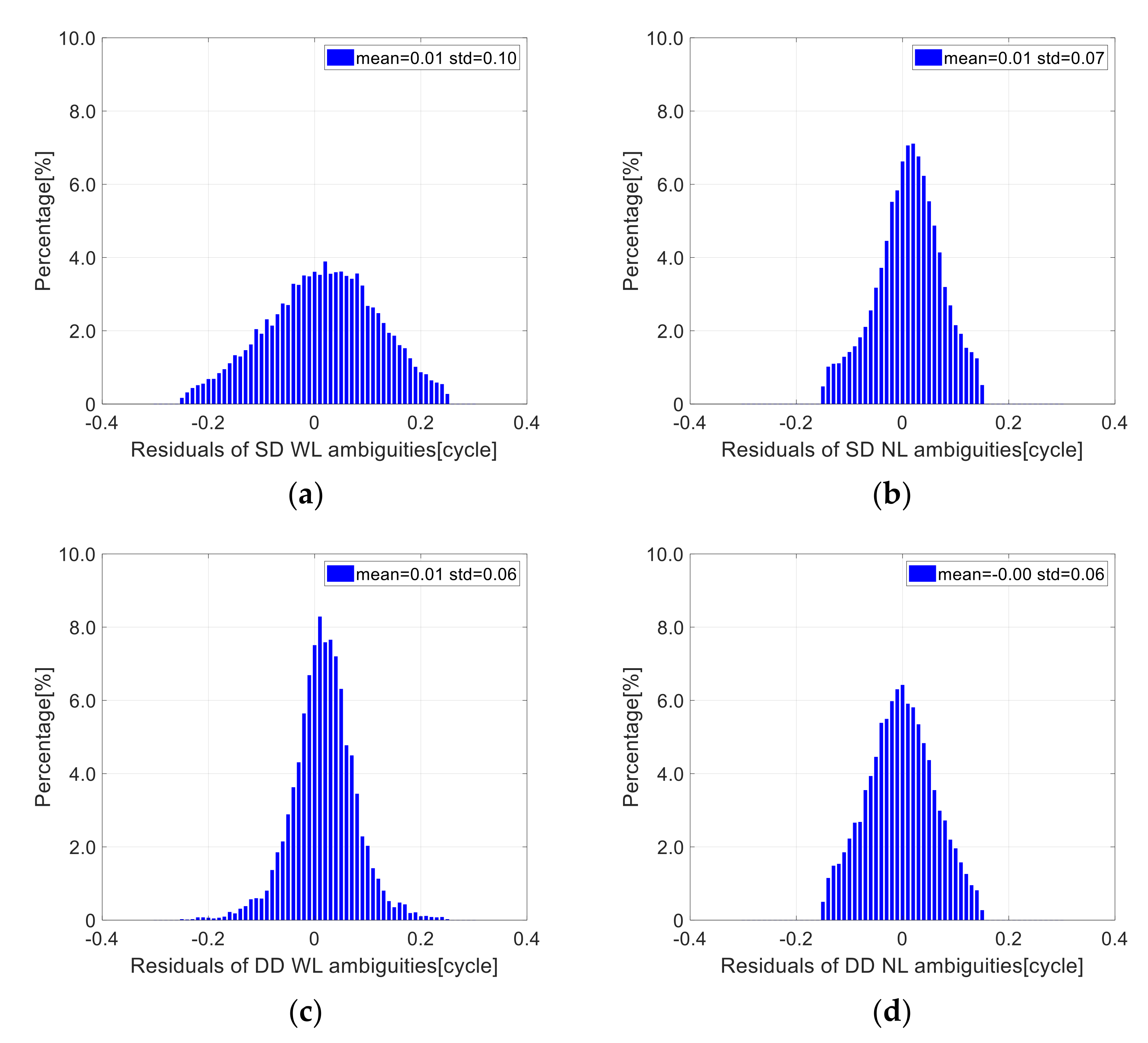
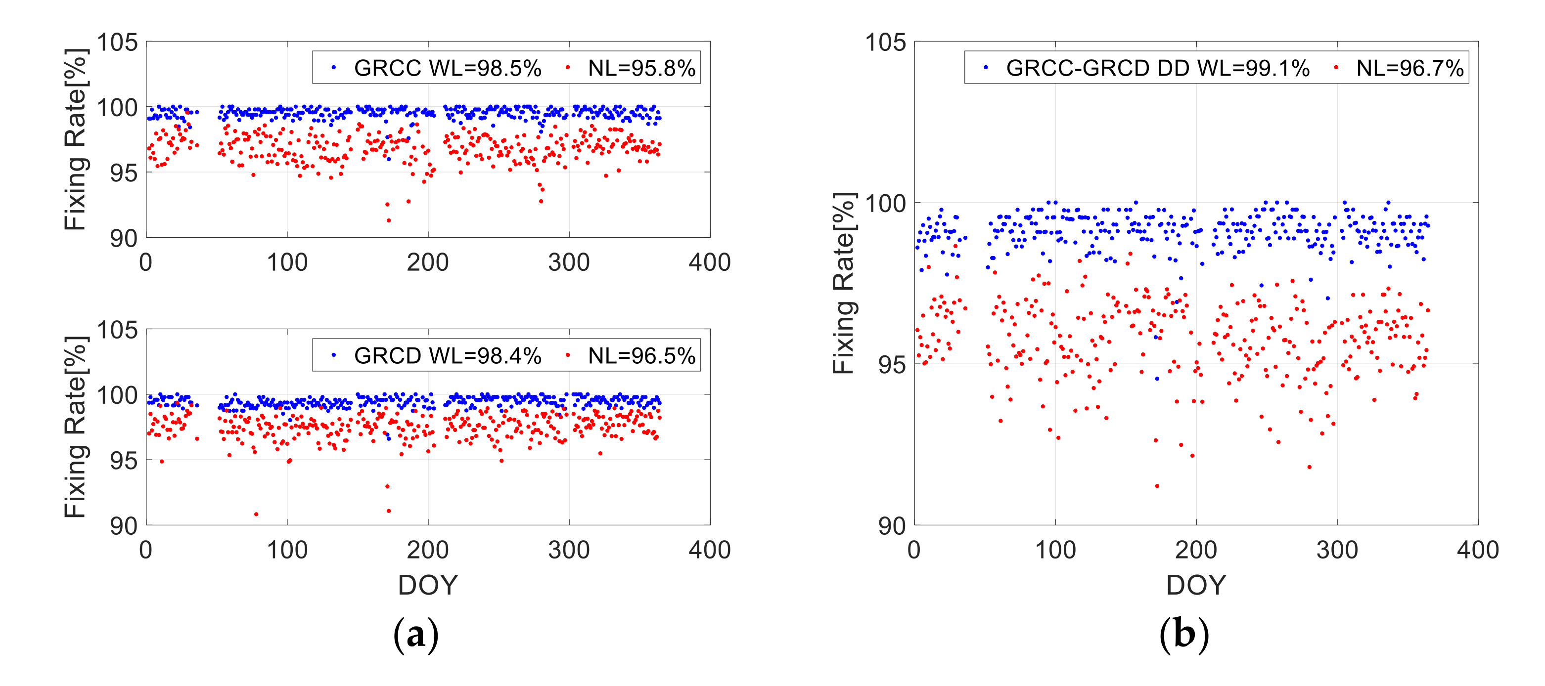
4.2.1. Ambiguity Resolution Results
4.2.2. Single Satellite Orbit Validation
4.2.3. Baseline Validation
5. Discussions
6. Conclusions
Author Contributions
Funding
Data Availability Statement
Acknowledgments
Conflicts of Interest
References
- Bertiger, W.; Bar-Sever, Y.; Christensen, E.; Davis, E.; Guinn, J.; Haines, B.; Ibanez-Meier, R.; Jee, J.; Lichten, S.; Melbourne, W.; et al. GPS precise tracking of TOPEX/POSEIDON: Results and implications. J. Geophys. Res. 1994, 99, 24449–24464. [Google Scholar] [CrossRef]
- Tapley, B.D.; Ries, J.C.; Davis, G.W.; Eanes, R.J.; Schutz, B.E.; Shum, C.K.; Watkins, M.M.; Marshall, J.A.; Nerem, R.S.; Putney, B.H.; et al. Precision orbit determination for TOPEX/POSEIDON. J. Geophys. Res. 1994, 99, 24383–24404. [Google Scholar] [CrossRef]
- Wu, S.C.; Yunck, T.P.; Thornton, C.L. Reduced-dynamic technique for precise orbit determination of low earth satellites. J. Guid. Control Dyn. 1991, 14, 24–30. [Google Scholar] [CrossRef]
- Jäggi, A.; Hugentobler, U.; Beutler, G. Pseudo-Stochastic Orbit Modeling Techniques for Low-Earth Orbiters. J. Geod. 2006, 80, 47–60. [Google Scholar] [CrossRef] [Green Version]
- Dow, J.M.; Neilan, R.E.; Gendt, G. The International GPS Service: Celebrating the 10th anniversary and looking to the next decade. Adv. Space Res. 2005, 36, 320–326. [Google Scholar] [CrossRef]
- Jäggi, A.; Hugentobler, U.; Bock, H.; Beutler, G. Precise orbit determination for GRACE using undifferenced or doubly differenced GPS data. Adv. Space Res. 2007, 39, 1612–1619. [Google Scholar] [CrossRef]
- Hackel, S.; Montenbruck, O.; Steigenberger, P.; Balss, U.; Gisinger, C.; Eineder, M. Model improvements and validation of TerraSAR-X precise orbit determination. J. Geod. 2017, 91, 547–562. [Google Scholar] [CrossRef]
- Van den Ijssel, J.; Visser, P.; Patiño Rodriguez, E. Champ precise orbit determination using GPS data. Adv. Space Res. 2003, 31, 1889–1895. [Google Scholar] [CrossRef]
- Kang, Z.; Tapley, B.D.; Bettadpur, S.; Ries, J.C.; Nagel, P.; Pastor, R. Precise orbit determination for the GRACE mission using only GPS data. J. Geod. 2006, 80, 322–331. [Google Scholar] [CrossRef]
- Luthcke, S.B.; Zelensky, N.P.; Rowlands, D.D.; Lemoine, F.G.; Williams, T.A. The 1-Centimeter Orbit: Jason-1 Precision Orbit Determination Using GPS, SLR, DORIS, and Altimeter Data Special Issue: Jason-1 Calibration/Validation. Mar. Geod. 2003, 26, 399–421. [Google Scholar] [CrossRef]
- Bertiger, W.; Desai, S.D.; Dorsey, A.; Haines, B.J.; Harvey, N.; Kuang, D.; Sibthorpe, A.; Weiss, J.P. Sub-centimeter precision orbit determination with GPS for ocean altimetry. Mar. Geod. 2010, 33, 363–378. [Google Scholar] [CrossRef]
- Bock, H.; Jäggi, A.; Meyer, U.; Visser, P.; van den IJssel, J.; van Helleputte, T.; Heinze, M.; Hugentobler, U. GPS-derived orbits for the GOCE satellite. J. Geod. 2011, 85, 807–818. [Google Scholar] [CrossRef] [Green Version]
- Bock, H.; Jäggi, A.; Beutler, G.; Meyer, U. GOCE: Precise orbit determination for the entire mission. J. Geod. 2014, 88, 1047–1060. [Google Scholar] [CrossRef]
- Peter, H.; Jäggi, A.; Fernández, J.; Escobar, D.; Ayuga, F.; Arnold, D.; Wermuth, M.; Hackel, S.; Otten, M.; Simons, W.; et al. Sentinel-1A-First precise orbit determination results. Adv. Space Res. 2017, 60, 879–892. [Google Scholar] [CrossRef]
- Montenbruck, O.; Hackel, S.; Jäggi, A. Precise orbit determination of the Sentinel-3A altimetry satellite using ambiguity-fixed GPS carrier phase observations. J. Geod. 2018, 92, 711–726. [Google Scholar] [CrossRef] [Green Version]
- Guo, J.Y.; Kong, Q.; Qin, J.; Sun, Y. On precise orbit determination of HY-2 with space geodetic techniques. Acta Geophys. 2013, 61, 752–772. [Google Scholar] [CrossRef]
- Li, M.; Li, W.; Shi, C.; Jiang, K.; Guo, X.; Dai, X.; Meng, X.; Yang, Z.; Yang, G.; Liao, M. Precise orbit determination of the Fengyun-3C satellite using onboard GPS and BDS observations. J. Geod. 2017, 91, 1313–1327. [Google Scholar] [CrossRef] [Green Version]
- Li, X.; Zhang, K.; Meng, X.; Zhang, W.; Zhang, Q.; Zhang, X.; Li, X. Precise Orbit Determination for the FY-3C Satellite Using Onboard BDS and GPS Observations from 2013, 2015, and 2017. Engineering 2019, 6, 904–912. [Google Scholar] [CrossRef]
- Kroes, R.; Montenbruck, O.; Bertiger, W.; Visser, P. Precise GRACE baseline determination using GPS. GPS Solut. 2005, 9, 21–31. [Google Scholar] [CrossRef]
- Zhao, Q.; Hu, Z.; Guo, J.; Li, M.; Ge, M. Precise relative orbit determination of twin GRACE satellites. Geo Spat. Inf. Sci. 2010, 13, 221–225. [Google Scholar] [CrossRef]
- Zhang, B.; Teunissen, P.J.G.; Odijk, D. A novel un-differenced PPP-RTK concept. J. Navig. 2011, 64, S180–S191. [Google Scholar] [CrossRef] [Green Version]
- Odijk, D.; Teunissen, P.J.G.; Zhang, B. Single-frequency integer ambiguity resolution enabled GPS precise point positioning. J. Surv. Eng. 2012, 138, 193–202. [Google Scholar] [CrossRef]
- De Jonge, P.J. A processing strategy for the application of the GPS in networks. Ph.D. Thesis, Delft University of Technology, Delft, The Netherlands, 1998. [Google Scholar]
- Teunissen, P.J.G.; Odijk, D.; Zhang, B. PPP-RTK: Results of CORS Network-Based PPP with Integer Ambiguity Resolution. J. Aeronaut. Astronaut. Aviat. Ser. 2010, 42, 223–230. [Google Scholar]
- Laurichesse, D.; Mercier, F.; Berthias, J.P.; Broca, P.; Cerri, L. Integer ambiguity resolution on undifferenced GPS phase measurements and its application to PPP and satellite precise orbit determination. Navigation 2009, 56, 135–149. [Google Scholar] [CrossRef]
- Loyer, S.; Perosanz, F.; Mercier, F.; Capdeville, H.; Marty, J.C. Zero-difference GPS ambiguity resolution at CNES–CLS IGS Analysis Center. J. Geod. 2012, 86, 991–1003. [Google Scholar] [CrossRef]
- Collins, P.; Bisnath, S.; Lahaye, F.; Héroux, P. Undifferenced GPS Ambiguity Resolution Using the Decoupled Clock Model and Ambiguity Datum Fixing. Navigation 2010, 57, 123–135. [Google Scholar] [CrossRef] [Green Version]
- Ge, M.; Gendt, G.; Rothacher, M.; Shi, C.; Liu, J. Resolution of GPS carrier-phase ambiguities in precise point positioning (PPP) with daily observations. J. Geod. 2008, 82, 389–399. [Google Scholar] [CrossRef]
- Geng, J.; Bock, Y. Triple-frequency GPS precise point positioning with rapid ambiguity resolution. J. Geod. 2013, 87, 449–460. [Google Scholar] [CrossRef]
- Teunissen, P.J.G. Zero Order Design: Generalized Inverses, Adjustment, the Datum Problem and S-Transformations. In Optimization and Design of Geodetic Networks; Grafarend, E., Sanso, F., Eds.; Springer: Berlin/Heidelberg, Germany, 1985; pp. 11–55. [Google Scholar]
- Teunissen, P.J.G.; Khodabandeh, A. Review and principles of PPP-RTK methods. J. Geod. 2015, 89, 217–240. [Google Scholar] [CrossRef]
- Bertiger, W.; Desai, S.D.; Haines, B.; Harvey, N.; Moore, A.W.; Owen, S.; Weiss, J.P. Single receiver phase ambiguity resolution with GPS data. J. Geod. 2010, 84, 327–337. [Google Scholar] [CrossRef]
- Arnold, D.; Schaer, S.; Villiger, A.; Dach, R.; Jäggi, A. Undifferenced ambiguity resolution for GPS-based precise orbit determination of low Earth orbiters using the new CODE clock and phase bias products. In Proceedings of the International GNSS Service Workshop 2018, Wuhan, China, 29 October–2 November 2018. [Google Scholar]
- Li, X.; Wu, J.; Zhang, K.; Li, X.; Xiong, Y.; Zhang, Q. Real-Time Kinematic Precise Orbit Determination for LEO Satellites Using Zero-Differenced Ambiguity Resolution. Remote Sens. 2019, 11, e2815. [Google Scholar] [CrossRef] [Green Version]
- Guo, X.; Geng, J.; Chen, X.; Zhao, Q. Enhanced orbit determination for formation flying satellites through integrated single and double difference GPS ambiguity resolution. GPS Solut. 2020, 24, 1–12. [Google Scholar] [CrossRef]
- Jäggi, A.; Dach, R.; Montenbruck, O.; Hugentobler, U.; Bock, H.; Beutler, G. Phase center modeling for LEO GPS receiver antennas and its impact on precise orbit determination. J. Geod. 2009, 83, 1145–1162. [Google Scholar] [CrossRef] [Green Version]
- Bock, H.; Jäggi, A.; Meyer, U.; Dach, R.; Beutler, G. Impact of GPS antenna phase center variations on precise orbits of the GOCE satellite. Adv. Space Res. 2011, 47, 1885–1893. [Google Scholar] [CrossRef]
- Van Den IJssel, J.; Encarnação, J.; Doornbos, E.; Visser, P. Precise science orbits for the Swarm satellite constellation. Adv. Space Res. 2015, 56, 1042–1055. [Google Scholar] [CrossRef]
- Montenbruck, O.; Garcia-Fernandez, M.; Yoon, Y.; Schön, S.; Jäggi, A. Antenna phase center calibration for precise positioning of LEO satellites. GPS Solut. 2008, 13, 23–34. [Google Scholar] [CrossRef]
- Haines, B.; Bar-Sever, Y.; Bertiger, W.; Desai, S.D.; Willis, P. One-centimeter orbit determination for Jason-1: New GPS-based strategies. Mar. Geod. 2004, 27, 299–318. [Google Scholar] [CrossRef]
- Yi, B.; Gu, D.; Ju, B.; Shao, K.; Zhang, H. Enhanced baseline determination for formation flying LEOs by relative corrections of phase center and code residual variations. Chin. J. Aeronaut. 2019, in press. [Google Scholar]
- Yuan, J.; Zhou, S.; Hu, X.; Yang, L.; Cao, J.; Li, K.; Liao, M. Impact of Attitude Model, Phase Wind-Up and Phase Center Variation on Precise Orbit and Clock Offset Determination of GRACE-FO and CentiSpace-1. Remote Sens. 2021, 13, e2636. [Google Scholar] [CrossRef]
- Xia, Y.; Liu, X.; Guo, J.; Yang, Z.; Qi, L.; Ji, B.; Chang, X. On GPS data quality of GRACE-FO and GRACE satellites: Effects of phase center variation and satellite attitude on precise orbit determination. Acta Geod. Geophys. 2021, 56, 93–111. [Google Scholar] [CrossRef]
- Wen, H.; Kruizinga, G.; Paik, M.; Landerer, F.; Bertiger, W.; Sakumura, C.; Bandikova, T.; Mccullough, C. Technical Report JPL D-56935: Grace-Fo Level-1 Data Product User Handbook; Jet Propulsion Laboratory: Pasadena, CA, USA, 2019. [Google Scholar]
- Tapley, B.D.; Bettadpur, S.; Watkins, M.M.; Reigber, C. The gravity recovery and climate experiment: Mission overview and early results. Geophys. Res. Lett. 2004, 31. [Google Scholar] [CrossRef] [Green Version]
- Dragon, K. Technical Report JPL D-71781: GRACE Follow-On Mission Plan; Jet Propulsion Laboratory: Pasadena, CA, USA, 2015. [Google Scholar]
- Liu, J.; Ge, M. PANDA software and its preliminary result of positioning and orbit determination. Wuhan Univ. J. Nat. Sci. 2003, 8, 603–609. [Google Scholar]
- Berger, C.; Biancale, R.; Ill, M.; Barlier, F. Improvement of the empirical thermospheric model DTM: DTM94-A comparative review of various temporal variations and prospects in space geodesy applications. J. Geod. 1998, 72, 161–179. [Google Scholar] [CrossRef]
- Förste, C.; Bruinsma, S.L.; Shako, R.; Marty, J.C.; Flechtner, F.; Abrikosov, O.; Dahle, C.; Lemoine, J.M.; Neumayer, K.H.; Biancale, R.; et al. EIGEN-6—A new combined global gravity field model including GOCE data from the collaboration of GFZ-Potsdam and GRGS Toulouse. In Proceedings of the EGU General Assembly, Vienna, Austria, 3–8 April 2011. [Google Scholar]
- Petit, G.; Luzum, B.; Al, E. IERS Conventions. IERS Tech. Note 2010, 36, 1–95. [Google Scholar]
- Lyard, F.; Lefevre, F.; Letellier, T.; Francis, O. Modeling the global ocean tides: Modern insights from FES2004. Ocean Dyn. 2006, 56, 394–415. [Google Scholar] [CrossRef]
- Desai, S.D. Observing the pole tide with satellite altimetry. J. Geophys. Res. 2002, 107, 1–13. [Google Scholar] [CrossRef]
- Wu, J.T.; Wu, S.C.; Hajj, G.A.; Bertiger, W.I.; Lichten, S.M. Effects of antenna orientation on GPS carrier phase. Manuscr. Geod. 1993, 18, 91–98. [Google Scholar]
- Meehan, T.; Esterhuizen, S.; Franklin, G.; Tien, J.; Young, L.; Bachman, B.; Munson, T.; Robison, D.; Stecheson, T. Development status of NASA’s TriG GNSS science instrument. In Proceedings of the International Radio Occultation Working Group (IROWG-2), Estes Park, CO, USA, 28 March–3 April 2012. [Google Scholar]
- Schaer, S.; Villiger, A.; Arnold, D.; Dach, R.; Prange, L.; Jäggi, A. The CODE ambiguity-fixed clock and phase bias analysis products: Generation, properties, and performance. J. Geod. 2021, 95, 1–25. [Google Scholar] [CrossRef]
- Villiger, A.; Schaer, S.; Dach, R.; Prange, L.; Sušnik, A.; Jäggi, A. Determination of GNSS pseudo-absolute code biases and their long-term combination. J. Geod. 2019, 93, 1487–1500. [Google Scholar] [CrossRef]
- Blewitt, G. Carrier phase ambiguity resolution for the Global Positioning System applied to geodetic baselines up to 2000 km. J. Geophys. Res. Solid Earth 1989, 94, 10187–10203. [Google Scholar] [CrossRef] [Green Version]
- Jin, B.; Chen, S.; Li, D.; Takka, E.; Li, Z.; Qu, P. Ionospheric correlation analysis and spatial threat model for SBAS in China region. Adv. Space Res. 2020, 66, 2873–2887. [Google Scholar] [CrossRef]
- Teunissen, P.J.G. GNSS Precise Point Positioning. In Position, Navigation, and Timing Technologies in the 21st Century: Integrated Satellite Navigation, Sensor Systems, and Civil Applications, 1st ed.; Morton, Y.J., van Diggelen, F., Spilker, J.J., Jr., Parkinson, B.W., Lo, S., Gao, G., Eds.; Wiley-IEEE Press: Hoboken, NJ, USA, 2021; Volume 1, pp. 503–528. [Google Scholar]
- Hatch, R. The synergism of GPS Code and carrier measurements. In Proceedings of the Third International Symposium on Satellite Doppler Positioning, Physical Sciences Laboratory of New Mexico State University, Las Cruces, NM, USA, 8–12 February 1982; pp. 1213–1231. [Google Scholar]
- Melbourne, W. The Case for Ranging in GPS Based Geodetic Systems. In Proceedings of the 1st International Symposium on Precise Positioning with the Global Positioning System, Rockville, MD, USA, 15–19 April 1985; pp. 373–386. [Google Scholar]
- Wubbena, G. Software developments for geodetic positioning with GPS using TI 4100 code and carrier measurements. In Proceedings of the 1st International Symposium on Precise Positioning with the Global Positioning System, Rockville, MD, USA, 15–19 April 1985; pp. 403–412. [Google Scholar]
- Geng, J.; Chen, X.; Pan, Y.; Zhao, Q. A modified phase clock/bias model to improve PPP ambiguity resolution at Wuhan University. J. Geod. 2019, 93, 2053–2067. [Google Scholar] [CrossRef]
- Teunissen, P.J. Carrier phase integer ambiguity resolution. In Springer Handbook of Global Navigation Satellite Systems, 1st ed.; Teunissen, P., Montenbruck, O., Eds.; Springer: Berlin/Heidelberg, Germany, 2017; pp. 661–685. [Google Scholar]
- Dong, D.; Bock, Y. Global positioning system network analysis with phase ambiguity resolution applied to crustal deformation studies in California. J. Geophys. Res. 1989, 94, 3949–3966. [Google Scholar] [CrossRef]
- Ge, M.; Gendt, G.; Dick, G.; Zhang, F.P. Improving carrier-phase ambiguity resolution in global GPS network solutions. J. Geod. 2005, 79, 103–110. [Google Scholar] [CrossRef]
- Teunissen, P.J.G. The parameter distributions of the integer GPS model. J. Geod. 2002, 76, 41–48. [Google Scholar] [CrossRef] [Green Version]
- Kang, Z.; Bettadpur, S.; Nagel, P.; Save, H.; Poole, S.; Pie, N. GRACE-FO precise orbit determination and gravity recovery. J. Geod. 2020, 94, 85. [Google Scholar] [CrossRef]
- Gu, D.; Ju, B.; Liu, J.; Tu, J. Enhanced GPS-based GRACE baseline determination by using a new strategy for ambiguity resolution and relative phase center variation corrections. Acta Astronaut. 2017, 138, 176–184. [Google Scholar] [CrossRef]
- Geng, J.; Yang, S.; Guo, J. Assessing IGS GPS/Galileo/BDS-2/BDS-3 phase bias products with PRIDE PPP-AR. Satell. Navig. 2021, 2, 1–15. [Google Scholar] [CrossRef]
- Montenbruck, O.; Hackel, S.; Wermuth, M.; Zangerl, F. Sentinel-6A precise orbit determination using a combined GPS/Galileo receiver. J. Geod. 2021, 95, 109. [Google Scholar] [CrossRef]


| Parameter | Description |
|---|---|
| Background force models | |
| Static gravity field model | EIGEN_06C (130 × 130) [49] |
| Solid earth and pole tides | IERS Conventions 2010 [50] |
| Ocean tides | FES2004 (30 × 30) [51] |
| Ocean pole tides | Desai [52] (30 × 30) |
| Third body perturbations | JPL’s DE405 |
| General relativistic effects | IERS Conventions 2010 [50] |
| Solar radiation pressure | Macro model [44] |
| Atmospheric drag | Macro model [44], DTM94 [48] |
| Input data and products | |
| GPS Observations | Undifferenced IF code and carrier phase |
| Sample interval | 10 s |
| Elevation mask | 0° |
| GPS orbit | CODE’s final GPS orbit |
| GPS clock and hardware bias | CODE’s 5 s clock and OSB products |
| GPS antenna correction | igs14.atx |
| GRACE-FO antenna correction | PCO applied [44] |
| Phase wind-up | Applied [53] |
| Gravitational bending | IERS Conventions 2010 [50] |
| Relativistic correction | IERS Conventions 2010 [50] |
| Estimated parameters | |
| Initial state vector | Position and velocity per satellite per arc |
| Atmospheric drag coefficient | One per orbital resolution |
| Scale coefficient of solar radiation pressure | One per satellite per arc |
| Empirical along- and cross-track accelerations | 1-CPR accelerations per orbital resolution |
| Receiver clock errors | Epoch wise |
| Carrier phase ambiguities | One per satellite tracking pass |
| Satellite | GPS Antenna PCO/m | SLR Reflector/m | ||||
|---|---|---|---|---|---|---|
| X | Y | Z | X | Y | Z | |
| GRCC | 0.26023 | −0.00128 | −0.47697 | 0.60000 | 0.32750 | 0.22080 |
| GRCD | 0.26004 | −0.00107 | −0.47618 | 0.60000 | 0.32750 | 0.22080 |
| Solution | Satellite | Orbit | No PCV/mm | With PCV/mm | Improvement |
|---|---|---|---|---|---|
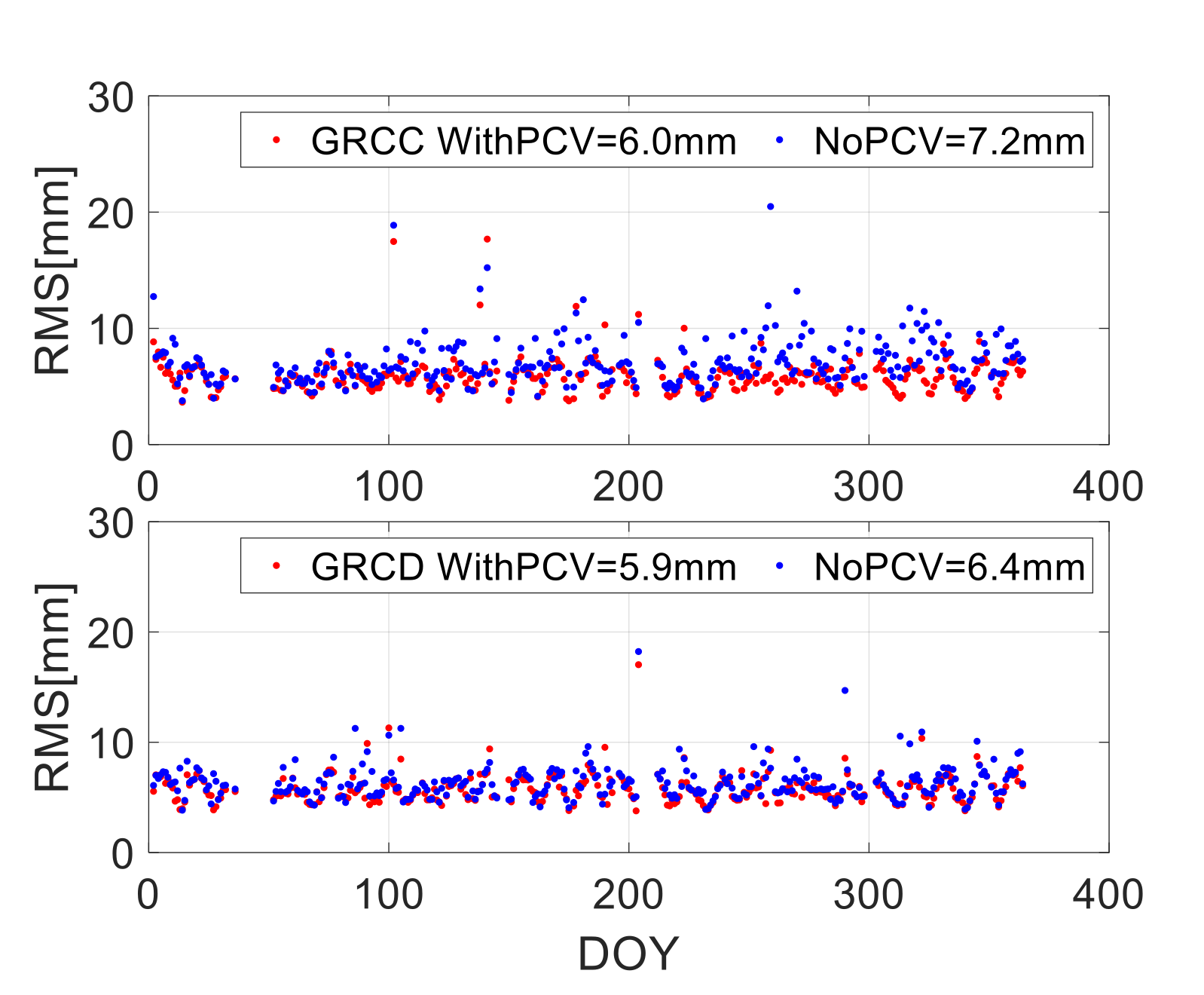
| SD AR Solution | GRCC | Along-track | 7.2 | 6.0 | 16.7% |
| Cross-track | 6.2 | 6.2 | 0 | ||
| Radial | 5.2 | 5.1 | 1.9% | ||
| GRCD | Along-track | 6.4 | 5.9 | 7.8% | |
| Cross-track | 6.3 | 6.1 | 3.2% | ||
| Radial | 5.1 | 5.1 | 0 | ||
| DD AR Solution | GRCC | Along-track | 9.5 | 8.3 | 12.6% |
| Cross-track | 6.5 | 6.4 | 1.5% | ||
| Radial | 5.8 | 5.6 | 3.4% | ||
| GRCD | Along-track | 8.8 | 8.1 | 8.0% | |
| Cross-track | 6.4 | 6.3 | 1.6% | ||
| Radial | 5.7 | 5.5 | 3.5% |
| Satellite | Orbit | Solutions/mm | Improvement | |||
|---|---|---|---|---|---|---|
| FA | DD AR | SD AR | DD AR | SD AR | ||
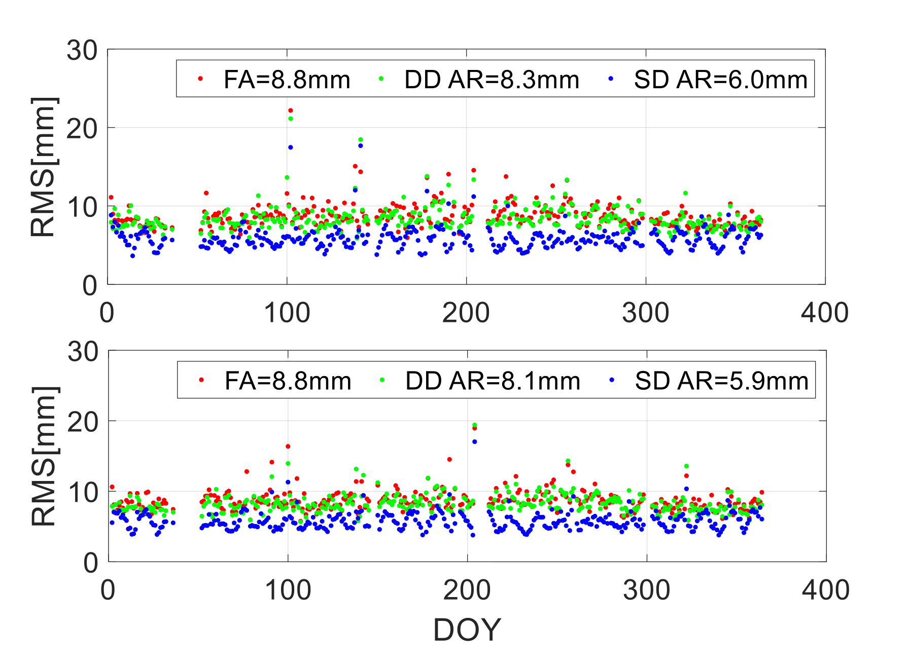
| GRCC | Along-track | 8.8 | 8.3 | 6.0 | 5.7% | 31.8% |
| Cross-track | 6.7 | 6.4 | 6.2 | 4.5% | 7.5% | |
| Radial | 6.0 | 5.6 | 5.1 | 6.7% | 15.0% | |
| GRCD | Along-track | 8.8 | 8.1 | 5.9 | 8.0% | 33.0% |
| Cross-track | 6.7 | 6.3 | 6.1 | 6.0% | 9.0% | |
| Radial | 5.9 | 5.5 | 5.1 | 6.8% | 13.6% | |
Publisher’s Note: MDPI stays neutral with regard to jurisdictional claims in published maps and institutional affiliations. |
© 2021 by the authors. Licensee MDPI, Basel, Switzerland. This article is an open access article distributed under the terms and conditions of the Creative Commons Attribution (CC BY) license (https://creativecommons.org/licenses/by/4.0/).
Share and Cite
Jin, B.; Li, Y.; Jiang, K.; Li, Z.; Chen, S. GRACE-FO Antenna Phase Center Modeling and Precise Orbit Determination with Single Receiver Ambiguity Resolution. Remote Sens. 2021, 13, 4204. https://doi.org/10.3390/rs13214204
Jin B, Li Y, Jiang K, Li Z, Chen S. GRACE-FO Antenna Phase Center Modeling and Precise Orbit Determination with Single Receiver Ambiguity Resolution. Remote Sensing. 2021; 13(21):4204. https://doi.org/10.3390/rs13214204
Chicago/Turabian StyleJin, Biao, Yuqiang Li, Kecai Jiang, Zhulian Li, and Shanshan Chen. 2021. "GRACE-FO Antenna Phase Center Modeling and Precise Orbit Determination with Single Receiver Ambiguity Resolution" Remote Sensing 13, no. 21: 4204. https://doi.org/10.3390/rs13214204
APA StyleJin, B., Li, Y., Jiang, K., Li, Z., & Chen, S. (2021). GRACE-FO Antenna Phase Center Modeling and Precise Orbit Determination with Single Receiver Ambiguity Resolution. Remote Sensing, 13(21), 4204. https://doi.org/10.3390/rs13214204