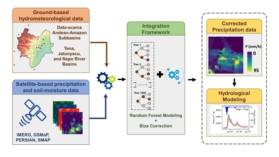
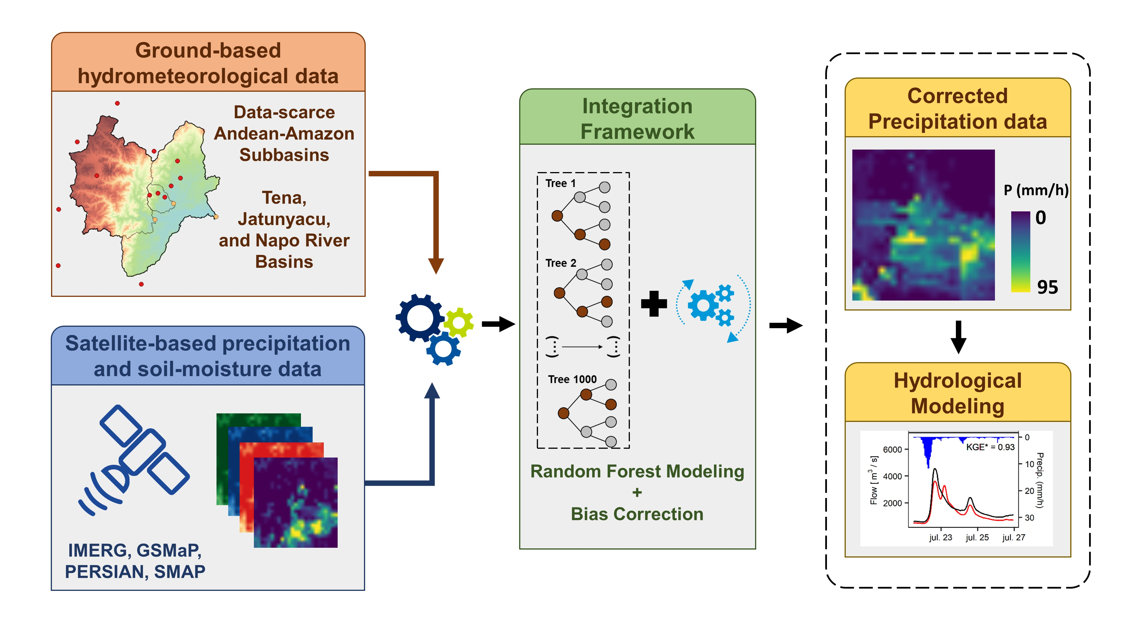
Improving Hourly Precipitation Estimates for Flash Flood Modeling in Data-Scarce Andean-Amazon Basins: An Integrative Framework Based on Machine Learning and Multiple Remotely Sensed Data

Abstract

Accurate estimation of spatiotemporal precipitation dynamics is crucial for flash flood forecasting; however, it is still a challenge in Andean-Amazon sub-basins due to the lack of suitable rain gauge networks. This study proposes a framework to improve hourly precipitation estimates by integrating multiple satellite-based precipitation and soil-moisture products using random forest modeling and bias correction techniques. The proposed framework is also used to force the GR4H model in three Andean-Amazon sub-basins that suffer frequent flash flood events: upper Napo River Basin (NRB), Jatunyacu River Basin (JRB), and Tena River Basin (TRB). Overall, precipitation estimates derived from the framework (BC-RFP) showed a high ability to reproduce the intensity, distribution, and occurrence of hourly events. In fact, the BC-RFP model improved the detection ability between 43% and 88%, reducing the estimation error between 72% and 93%, compared to the original satellite-based precipitation products (i.e., IMERG-E/L, GSMAP, and PERSIANN). Likewise, simulations of flash flood events by coupling the GR4H model with BC-RFP presented satisfactory performances (KGE* between 0.56 and 0.94). The BC-RFP model not only contributes to the implementation of future flood forecast systems but also provides relevant insights to several water-related research fields and hence to integrated water resources management of the Andean-Amazon region.

1. Introduction

Accurate estimation of spatiotemporal precipitation dynamics is crucial for several hydrological purposes, especially for operational flash flood forecasting [1,2]. Conventional approaches to estimate the precipitation patterns require rain gauge information. However, the spatial distribution of rain gauges strongly influences the uncertainty of precipitation estimates [3,4]. This implies important limitations over areas with complex topography, as in the case of the Andean-Amazon sub-basins, where implementing a suitable rain gauge density is often difficult and cost-prohibitive. In recent years, satellite-based precipitation products (hereafter SPPs) have been constituted as an alternative to overcome this limitation [5,6]. Nevertheless, SPPs present multiple sources of random and systematic errors associated with retrieval algorithms, sampling time steps, detection ability, among others [7,8].

In this regard, several studies have proposed different methods to improve the accuracy of SPPs and use them for forcing precipitation in hydrological models [9,10,11,12]. Most of these studies have focused on bias correction by statistical techniques and regression- based downscaling using land surface characteristics [13,14,15,16,17,18,19,20]. However, these correction methods still present several issues at high spatial (i.e., <10 km) and temporal (i.e., hourly) resolutions [21]. Thus, their applicability for hydrological modeling in fast-response basins is limited [22,23]. To address these issues, recent investigations have proposed various correction methods based on machine learning. For instance, Le et al. [24] developed a framework to correct daily and sub-daily SPPs by convolutional neural networks, obtaining higher performances than classical correction methods. Likewise, Chivers et al. [25] and Wolfensberger et al. [26] suggested a combination of random forest modeling with classical bias correction methods to improve hourly precipitation estimates derived from SPPs. However, the latter method focuses on the individual correction of SPPs without considering the valuable information that could be better captured by other precipitation products.

In contrast, Baez et al. [27] and Kolluru et al. [28] proposed merging multiples SPPs with rain gauge data and geographical features by random forest modeling. This method extracts the most relevant information from each SPP and combines it to maximize the accuracy of precipitation estimates. Results obtained with this method showed significant increases in performances of precipitation estimates (greater than 60%) compared to using isolated SPPs [27,28]. Further studies have indicated the combination of SPPs with satellite-based soil-moisture products (hereafter SMPs) also provides relevant insights to improve the accuracy of precipitation estimates [29,30,31,32]. In fact, soil-moisture information have proven to be an excellent indicator of the precipitation occurrence, especially at high temporal scales [33].

Although the integration of multiple SPPs and SMPs by machine learning provides an unprecedented opportunity to better estimate the precipitation dynamics in data-scarce regions, its applicability has not been evaluated in the Andean-Amazon basins. A representative Andean-Amazon basin is the upper part of the Napo River Basin, as it presents a complex topography and fast hydrological responses. Given its characteristics, the upper Napo River Basin is prone to recurrent flash floods [34,35]. In spite of this, no operational hydrological modeling and hence flood forecasting systems have been implemented in the region due to the scarce rain gauge data and hence suitable spatiotemporal precipitation estimates.

To address this problem, this study aims to propose an integrative framework for improving the estimation of spatiotemporal precipitation dynamics (i.e., intensity, distribution, and occurrence) at an hourly scale in the upper Napo River Basin. The framework combines multiple SPPs and SMPs with ground observed data and geographical features using random forest modeling and bias correction methods. The potential use of the framework as forcing precipitation inputs for hydrological modeling was illustrated in three gauged sub-basins within the upper Napo River Basin that suffer continuous flood risk. This study might not only contribute to the development of flood forecasting systems, but also to several water-related research fields and hence to integrated water resources management in the Andean-Amazon region.

2. Study Area

The Napo River is an important tributary of the Amazon Basin (Figure 1a) providing a mean annual discharge of about 6300 m³/s. It covers a drainage area of 100,500 km², distributing among Ecuador (59.6%), Peru (40.0%), and Colombia (0.4%) (Figure 1b) [36]. This study focuses on the upper part of the Ecuadorian Napo River Basin (hereafter NRB), located between the Eastern Andes and the Amazonia foothills. The NRB covers 6095 km² above the H1156 hydrological station and presents steep slopes that descend from 5900 to 370 m.a.s.l. over only 100 km (Figure 1c) [37]. Due to this complex topography, the NRB presents a strong climate gradient. Along this climate gradient, several ecosystems can be found, from the higher to lower elevations: (i) paramo, (ii) mountain forest, and (iii) piedmont rainforest (Figure 1d).

The paramo is located in the western highlands of the NRB (above 3200 m.a.s.l.). It presents mean temperatures that range from 4 to 8 °C. The precipitation is influenced by moisture originated from both the Pacific and Atlantic oceans with annual accumulation that varies from 500 to 2000 mm [38,39]. In the paramo, the precipitation occurs mainly as drizzle (~0.1 mm/h) [40], however, rainfall events with high-relative intensities (60 mm/h) have been reported [38]. The mountain forest, instead, is a transitional region between the paramo and piedmont rainforest. Here, mean annual temperature varies from 12 to 20 °C and the annual precipitation ranges from 2000 to 4000 mm. In general, the precipitation mainly occurs by orographic and convective events, reaching maximum intensities up to ~85 mm/h [41].

The piedmont rainforest is located in the eastern lowlands of the NRB (i.e., below 900 m.a.s.l.). This region is dominated by a humid tropical climate with annual rainfall between 3500 and 5000 mm, and mean temperatures from 20 to 27 °C [42]. Overall, precipitation presents intensities from 20 to 40 mm/h. However, extreme events above 95 mm/h have been recorded [35]. The piedmont rainforest is the most critical region within the NRB as its soil-saturation conditions and strong precipitation regime generate frequent flooding. Indeed, nine flash floods with peak discharges above 6000 m³/s have been recorded near the NRB outlet during the last 12 years, affecting on average 8000 families per year [42,43,44].

In the NRB, there are two additional critical points that suffer recurrent flash floods, which are the outlets of the Tena River Basin (TRB) and Jatunyacu River Basin (JRB). The TRB drains 239 km² above the HI001 hydrological station in Tena City. The streamflow and baseflow average 24.4 m³/s and 8 m³/s, respectively [42]. In the last years, four flash floods have been registered in the TRB, reaching peak discharges above 1800 m³/s [35]. On the other hand, the JRB has a drainage area of 3128 km² above the H0721 hydrological station. According to this station, discharge averages 290 m³/s [45]. Since 2010, three flash floods with peak discharges above 2500 m³/s have been recorded near the JRB outlet [45,46].

3. Datasets and Methods

3.1. Data

3.1.1. Ground-Observed Precipitation and Streamflow Data

Hourly precipitation and streamflow data were obtained from 12 meteorological stations and 3 hydrological stations (Figure 1c) belonging to the Ikiam Hydrometeorological Service [42] and the National Institute of Meteorology and Hydrology of Ecuador [45,46]. The analysis period was from January 2016 to December 2020 (5 years). We chose this period due to the availability of hourly data within the study area. Prior to this study, a data quality analysis was performed to find and remove outliers using the graphical method described in Chebana et al. [47]. It consists in visualizing data by a rainbow plot and then identifying outliers using bagplots and highest-density region boxplots.

3.1.2. Satellite-Based Data

Satellite-based precipitation data were obtained from the Integrated Multi-Satellite Retrievals for GPM Early Run (IMERG-E) and Late Run (IMERG-L) [48,49], the Global Satellite Mapping of Precipitation (GSMAP) [50,51], and the Precipitation Estimation from Remotely Sensed Information using Artificial Neural Networks—Cloud Classification System (PERSIANN-CCS) [52]. We focus on these products as they are widely used for flash flood analysis [53,54,55,56] due to their high spatiotemporal resolutions and low latency (

Table 1. General information of satellite-based precipitation and soil-moisture data used in this study.

Satellite Product	Spatial Resolution	Temporal Resolution	Latency	Download Website 1
GPM IMERG-E	0.10°	0.5 h	6 h	https://giovanni.gsfc.nasa.gov/giovanni/
GPM IMERG-L	0.10°	0.5 h	12 h	https://giovanni.gsfc.nasa.gov/giovanni/
GSMAP	0.10°	1 h	1 h	https://sharaku.eorc.jaxa.jp/GSMaP/
PERSIANN-CCS	0.04°	1 h	1 h	https://chrsdata.eng.uci.edu/
SMAP L4-SM	0.09°	3 h	7 d	https://nsidc.org/data/SPL4SMGP/versions/5

¹ Accessed on 7 March 2021.

). Likewise, soil moisture data at surface level (SM) and root zone (RM), as well their temporal variation (i.e., ΔSM and ΔRM), were derived from the Soil Moisture Active-Passive Satellite Mission (SMAP L4-SM product).

3.2. Integration of Satellite-Based Products

To achieve a new high-resolution and fitting precipitation product over the NRB, the proposed framework was implemented into three steps (Figure 2): (i) preprocessing, (ii) random forest precipitation modeling, and (iii) postprocessing or bias correction. Further details of the framework are described as follows.

3.2.1. Preprocessing

To ensure spatial consistency, the SPPs and SMPs were resampled to 4 km (the highest resolution provided by the precipitation products) using the bilinear method, following recommendations presented in Baez et al. [27]. Temporal consistency was obtained by aggregating or disaggregating the satellite-based products to hourly intervals [57]. The SPPs were aggregated by simple sum, whereas SMPs were disaggregated using the proximal interpolation method [58].

Since topographic features and temporal variability play an important role in precipitation patterns [59], variables such as altitude (ALT), monthly variability (MON), and hourly variability (HOUR) were considered as ancillary covariates. Altitude was derived from the Shuttle Radar Topography Mission (SRTM v4.1 90m) which was previously resampled to 4 km. Once the covariates were on the same temporal and spatial scales, we generated a data matrix joining information from the SPPs and SMPs, ancillary covariates, and ground-observed precipitation of each meteorological station. Data extraction was performed by point-to-pixel scale (Figure 2).

3.2.2. Random Forest Precipitation (RFP) Modeling

To integrate the SPPs and SMPs with ground-observed precipitation data and the ancillary covariates, we used a random forest (RF) model as the core of the framework.

A RF model is a machine learning technique that combines a large number of regression trees [60]. Each tree is generated with random data subsets sampled independently. These random data subsets are permuted at each splitting node for each tree, which reduces overfitting and improves the strength of predictions [61]. Thus, the error converges to the minimum possible as the number of trees increases within the forest. Given that the RF model generates a prediction for each tree, the final output is the average of all predictions.

We implemented the RF model using the R package “randomForest” [62]. With this package, the RF model requires two parameters: the number of regression trees (ntree) and the number of predictor variables at each node (ntry). We established ntree = 1000 and ntry = 4, following recommendations presented in Wolfensberger et al. [26]. The k-fold cross-validation method (k = 10) was proposed for model training. For this, the input data was previously divided into training (70%) and testing (30%) subsets.

Additionally, a variable importance analysis was simultaneously performed with the model training, calculating the percentage increase in mean square error (%IncMSE) for out-of-bag samples after permutating each covariate [59]. High %IncMSE values correspond to high importance and hence greatest influence on the precipitation prediction. Since the RF model generates a new gridded precipitation product, we called it random forest precipitation (hereafter RFP).

3.2.3. Postprocessing: The Bias-Corrected Random Forest Precipitation (BC-RFP)

Given the RFP model could present systematic bias due to the error associated with satellite-based covariates and the resampling process [59], we carried out a bias correction by the gamma quantile mapping method (GQM). This parametric method corrects precipitation assuming a gamma distribution. Thus, GQM nonlinearly corrects the mean, variance, intensities, and frequencies of wet hours [63]. A further description of this method is presented in Fang et al. [64]. The bias correction was performed considering the three main ecosystems of the study area. Note that each ecosystem presents a specific precipitation regime (see Section 2).

3.3. Statistical Criteria for Performance Assessment

Performance of precipitation estimates derived from the integration framework (i.e., RFP and BC-RFP) was assessed by comparison with observed precipitation data at a point-to-pixel scale. For this, we used three common continuous-statistic metrics: root mean square error (RMSE), correlation coefficient (R), and Kling–Gupta efficiency (KGE). Furthermore, three categorical statistics were used to assess the precipitation detection ability: probability of detection (POD), false alarm ratio (FAR), and critical success index (CSI).

Likewise, the SPPs used as covariates in the integrative framework were previously assessed to determine a reference for the improvement reached by RFP and BC-RFP. Mathematical definitions and characteristics of the aforementioned statistical metrics are described in Appendix A 

Table A1. Statistical criteria used to evaluate the performance of the integrative framework that combine multiple SPPs and SMPs with observed precipitation data and spatiotemporal covariates.

Metric	Definition	Optimum Value	Range	Unit
RMSE	$\mathrm{RMSE}=\sqrt{\frac{{{\displaystyle \sum }}_{i=1}^n{\left(S_i-O_i\right)}^2}{n}}$	0	(0, Inf)	mm/h
CORR	$\mathrm{CORR}=\frac{cov \left(S, O\right)}{\sqrt{var\left(S\right)} \sqrt{var\left(O\right)}}$	1	(−1, 1)	-
KGE	$\mathrm{KGE}=1-\sqrt{{(\alpha -1)}^2+{\left(\beta -1\right)}^2+{\left(r-1\right)}^2}$	1	(−Inf, 1)	-
POD	$\mathrm{POD}=\frac{A}{A+B}$	1	(0, 1)	-
FAR	$\mathrm{FAR}=\frac{C}{A+C}$	0	(0, 1)	-
CSI	$\mathrm{CSI}=\frac{A}{A+B+C}$	1	(0, 1)	-

.

3.4. Hydrological Aplication

The bias-corrected estimates derived from the integrative framework (i.e., BC-RFP) were used as forcing precipitation inputs for the GR4H model. This hydrological model has been widely used for flash floods modeling due to its simple structure, low computing needs, and ability to simulate hourly streamflow [65,66]. Previous studies, such as Llauca et al. [67] and Espitia et al. [68], showed that the GR4H model can satisfactorily simulate the hydrological processes over the Andean-Amazon sub-basins. Details of the hydrological modeling process are described as follows.

3.4.1. Model Parameters and Inputs

The GR4H model has four free parameters that characterize the storage processes and unit hydrograph: X1, maximum capacity of moisture store (mm); X2, groundwater exchange coefficient (mm/h); X3, maximum capacity of the routing store (mm); and X4, base time of the unit hydrograph (h). A complete description of the model structure and equations are shown in Mathevet [65] and Bennett et al. [66]. The GR4H model requires precipitation and potential evapotranspiration (ETP) data as inputs. As previously mentioned, precipitation data were derived from the BC-RFP. ETP was calculated using the modified FAO Penman─Monteith method at hourly steps using the R package “water” [69,70], and interpolated along the study area with the Kriging method. For this, we used the meteorological data (temperature, relative humidity, solar radiation, and wind speed) provided by stations located in the study area.

3.4.2. Hydrological Modeling Setup

The GR4H model was calibrated and validated for the three study sub-basins: TRB, JRB, and NRB (Figure 1). We used the R package “airGR” [65,66] following a semi-distributed setting as shown in Figure A1.

Model calibration considered 40 months for the NRB and JRB (January 2016–March 2019), and 18 months for the TRB (July 2018–December 2019). Before this, we considered a warm-up period of six months to reduce the uncertainty associated with initial moisture conditions of the model. Model parameters were automatically calibrated by the shuffled complex evolution algorithm [71], using the nonparametric variant of the Kling─Gupta efficiency (KGE*) as the objective function [72]. We chose this metric as it provides better agreement between simulated and observed streamflow at sub-daily and hourly steps compared to the Nash─Sutcliffe efficiency [72,73]. The flow duration curve (FDC) and the percent bias (PBIAS) were also used to assess the model performance in term of streamflow distribution and model bias. The mathematical definition of the evaluation metrics is shown in

Table A2. Statistical criteria used to evaluate the performance of the GR4H model.

Metric	Definition	Optimum Value	Range	Unit
KGE*	${\mathrm{KGE}}^{*}=1-\sqrt{{(\alpha -1)}^2+{\left({\beta }_{NP}-1\right)}^2+{\left(r_{NP}-1\right)}^2}$	1	(−Inf, 1)	-
PBIAS	$\mathrm{PBIAS}= \frac{{{\displaystyle \sum }}_{i=1}^n{\left(S_i-O_i\right)}^{ }}{{{\displaystyle \sum }}_{i=1}^n{\left( O_i\right)}^{ }}$	0	(−1, 1)	-

.

Model validation consisted of evaluating the GR4H outputs using the optimal parameters obtained in the calibration step. To perform the validation, we used 20 months for the NRB and JRB (April 2019–December 2020), and 12 months for the TRB (January 2020–December 2020).

3.4.3. Flash Flood Event Analysis

The five last flash flood events produced within the study area (

Table 2. Information of the last five flash flood events produced within the study area.

Event	Start (Datetime)	Duration (h)	Peak Discharge (m3/s)
			TRB	JRB	NRB
1	2017-09-02 19:00	53	1896	1160	3570
2	2018-07-22 01:00	51	657	2579	4574
3	2019-05-25 20:00	28	242	1184	6407
4	2019-06-20 00:00	72	250	2659	6338
5	2020-05-01 00:00	80	593	896	8925
Streamflow threshold for flood events			210	2200	4500

) were used to assess the performance of the coupling of the BC-RFP and GR4H models during high flow conditions. These events were chosen based on:

• Records of the National Service for Risk Management of Ecuador [44].
• Streamflow thresholds defined by Hurtado et al. [35] and Lapo et al. [34] for flood events in the TRB, JRB, and NRB (Table 2).

For the event analysis, we focused on the differences between the simulated and observed behavior of four hydrograph aspects widely examined in flash flood modeling [74]:

• Streamflow dynamic or hydrograph shape.
• Peak discharge.
• Volume discharge.
• Peak timing.

4. Results and Discussion

4.1. Preliminary Evaluation of the SPPs

The SPPs used as covariates in the integration framework showed non-satisfactory performances within the study area (Figure 3). In terms of the RMSE, the SPPs presented errors that ranged between 0.6 and 3.3 mm/h. Compared to previous studies [75,76,77], these values could be considered acceptable. However, CORR and KGE metrics were below 0.4, indicating a poor agreement between SPPs and observed precipitation data. Similarly, detection performances (POD < 0.6, FAR > 0.5, CSI < 0.4) suggested that SSPs cannot correctly capture the hourly precipitation occurrence. These results agreed with several authors [67,68,69,70,71,72,73,74,75,76,77,78,79] who previously found important limitations in precipitation estimates of SSPs at fine temporal scales over complex topography regions, as in the case of the study area.

4.2. Variable Importance Analysis

The variable importance analysis revealed that all covariates, except PERSIANN, strongly influenced the performance of the integration framework as %IncMSE values ranged from 0.25 to 0.88 (Figure 4). The IMERG-E product and the soil-moisture change at root zone (ΔRM) were the most important covariates and hence those that contributed more information to precipitation estimates. Likewise, IMERG-L and soil moisture change at surface level (ΔSM) showed relatively high importance (%IncMSE > 50). These findings complied with those of Bhuiyan et al. [80,81], who discussed that the synergy among IMERG- and SMAP-derived soil-moisture products provides relevant insights to improve the fitting of precipitation patterns.

Monthly variability (MONTH) was the third most important predictor. However, its importance varied along the study area. Note that paramo does not present a strong precipitation seasonality [39,40], whereas the mountain forest and piedmont rainforest have the wettest season from March to July [82]. Altitude (ALT) and hourly variability (HOUR) showed similar importance. In general, both covariates are associated with the valley─mountain effect that generates convective precipitation events with high occurrence in the late afternoon and night along the study area [83].

As mentioned, PERSIANN was not a relevant covariate within the integration framework. This finding was consistent with the prior evaluation of SPPs (Figure 3), which indicated that PERSIANN was the worst performing product. In fact, this SPP presented no correlation with the observed data (CORR < 0.1) and the lowest detection skill (i.e., CSI < 0.12). As discussed Tan et al. [84], the low performance of PERSIANN is related to its low latency and hence lower processing compared to other SPPs. Note the PERSIANN product used in this study was derived from the cloud classification system that runs in real time.

4.3. Integration Framework Performance

The integration framework showed a high ability to capture the hourly precipitation within the study area (Figure 5). Precipitation estimates derived from RFP exhibited good performances for both training and testing periods (CORR ≈ 0.93, RMSE ≈ 0.77, and KGE ≈ 0.67). However, these preliminary results presented a systematic error, underestimating events with intensities greater than 15 mm/h (Figure 5a,c). As discussed by Zhang et al. [85], the RF algorithm uses the average of all prediction trees to generate model outputs. Therefore, it tends to underestimate extreme precipitation events. Nevertheless, this error was minimized in the postprocessing step by applying a bias correction using the GQM method (Figure 5b,d). As result, the corrected precipitation estimates (BC-RFP) showed notable improvements in accuracy and better captured the highest precipitation intensities (CORR > 0.95, RMSE < 0.65, and KGE > 0.83).

While the aforementioned results provide information about precipitation intensity performances, they do not clearly denote the ability of the integration framework to capture the occurrence of precipitation events. Capturing the precipitation occurrence is important because even small amounts of rainfall can affect the initial soil moisture conditions in the study area with subsequent impacts on the flash flood generation [86].

The precipitation detection ability of the BC-RFP model diminishes as the intensity threshold decreases, meaning that the BC-RFP model is less able to capture the correct magnitude of low-intensity events (Figure 6). Within the study area, low-intensity events (below 0.2 mm/h) mainly occur on the paramo. This denoted the difficulty of estimating precipitation at fine temporal scales over high-elevation regions [87]. For intensities between 2 and 50 mm/h, the precipitation detection ability (based on POD, FAR, and CSI) reaches the highest performances, suggesting that the BC-RFP model correctly estimates both intensity and occurrence of precipitation events in this precipitation range. Above 50 mm/h, the detection performance decreases slightly compared to precipitation events below 50 mm/h. However, these results suggested that BC-RFP presents a high potential to detect flash flood caused by heavy rainfalls (i.e., 50–100 mm/h).

Considering intensity thresholds altogether, the BC-RFP model showed satisfactory performances in detection metrics (POD = 0.67, FAR = 0.27, and CSI = 0.54). This indicates the proposed framework improved the detection ability between 43% and 88% compared to the original SPPs (i.e., IMERG-E/L, GSMAP, and PERSIANN). In fact, general performances reached by the BC-RFP model were similar to those reported by more complex methods that use RF models to correct and downscale the hourly precipitation estimates [25,26].

4.4. Spatial Consistency Analysis

As shown in Figure 7, the spatial distribution of annual precipitation obtained by the BC-RFP model was consistent with climate precipitation trends that characterize the Andean-Amazon region (see Section 2). No anomalous or out-of-trend pixels were found in the paramo and mountain forest regions. However, few pixels located in the lowest reaches of the NRB (piedmont rainforest) showed an important overestimation. While the long-term measurements in the aforementioned area indicate that annual precipitation does not exceed 5500 mm [88,89], the BC-RFP model showed values above 6500 mm/year. This can be explained by two reasons: (i) the SMAP-derived data exhibited the highest soil-moisture contents over the lowest reaches of the NRB, and (ii) the training of the integrative framework did not consider a rain gauge in this sector. Therefore, the BC-RFP model incorrectly interpreted these high moisture contents as more amounts of rainfall due to the lack of hourly precipitation data in the training set. Given that few pixels presented this problem, we considered they provided no significant impact in our hydrological modeling.

4.5. Calibration and Validation of the GR4H Model

The assessment of the BC-RFP model’s ability to force precipitation input for the GR4H model presented satisfactory performances (Figure 8). Overall, KGE* values between simulated and observed streamflows were above the acceptable threshold (KGE* > 0.5) [72]. Likewise, PBIAS showed scores below ±20%, indicating a good fitting [90]. The visual assessment based on the flow duration curve (FDC) revealed that the combination of the BC-RFP and GR4H models correctly captured the cumulative frequency of the streamflow distribution, except above the 95th percentile where the streamflow was underestimated.

In the TRB, the GR4H model showed the highest performances, reaching KGE* of 0.87 and 0.79 for calibration and validation, respectively (Figure 8a). These yields were higher than those reported by Espitia et al. [68], who previously implemented the GR4H model in the TRB. The main limitation faced by previous hydrological studies in the TRB was the lack of spatial precipitation data [35,68]. Our results partially overcame this limitation and corroborated that streamflow simulations of the TRB can be improved by the spatialization of the precipitation.

Regarding the JRB, streamflow simulations showed ~30% lower performance than that shown by the TRB, reaching KGE* values of 0.65 and 0.54 for calibration and validation, respectively (Figure 8b). FDCs revealed a high underestimation of streamflow distribution above 300 m³/s that was corroborated by PBIAS that shows a value of −18.2% for the validation period. This notable reduction in model performance is explained by the larger hydrological heterogeneity of the JRB produced by its complex topography and the transition between the paramo and the mountain forest. In fact, various studies such as Du et al. [91] and Liu et al. [92] have discussed that uncertainty on the parameter estimation increases considerably under these conditions. The error associated with low-intensity precipitation estimates produced in the paramo was another driver performance reduction in the JRB (see Section 4.3). Given the low ability of the BC-RFP model to detect drizzle events (>0.2 mm/h), the humidity conditions of the JRB may have been underestimated during most of the simulation time which affected the runoff generation [93].

Considering the whole study basin (NRB), the GR4H model showed KGE* values of about 0.54 ± 0.03. The streamflow was overestimated during calibration (PBIAS = 3.1%) and underestimated during the validation (PBIAS = −16.2%). Although this basin presented the lowest performances (Figure 8c), the FDC analysis indicated that high streamflows were better simulated compared to the JRB. This confirms that regardless of the overestimation problem occurring in lowest reaches of the NRB (see Section 4.4), the BC-RFP model better captured the high precipitation events in the piedmont rainforest compared to other regions within the study area. Note the piedmont rain forest presented the highest precipitation intensities and hence produced more runoff within the NRB [37].

4.6. Flood Event Analysis

As discussed in the previous section, streamflow simulations of the GR4H model underestimated high discharges. For the last five flash flood events that occurred in the TRB, JRB, and NRB (Figure 9), simulated peak flows were 3.8% to 47.8% lower than observed peak flows (

Table 3. Results of the event analysis considering the last five floods that occurred in the Tena River Basin (TRB), Jatunyacu River Basin (JRB), and upper Napo River Basin (NRB).

Event	Basin	Peak Flow (m3/s)			Runoff Volume (Hm3)			Difference in Peak Timing (h)
		Obs.	Sim.	Diff. (%)	Obs.	Sim.	Diff. (%)
1	TRB	1896	1379	−27.2	33.8	29.9	−11.5	0
	JRB	1160	2117	82.4	109.4	160.8	46.9	−3
	NRB	3570	3231	−9.5	245.5	333.7	35.9	2
2	TRB	657	365	−44.4	30.1	23.0	−23.6	0
	JRB	2579	1344	−47.8	270.3	198.0	−26.2	1
	NRB	4574	3614	−20.9	390.5	359.0	−8.1	1
3	TRB	242	258	6.5	8.7	5.8	−33.3	0
	JRB	1184	877	−25.9	60.2	73.0	21.2	12
	NRB	6407	5661	−11.6	276.2	240.4	−13.0	−1
4	TRB	250	241	−3.8	17.2	16.6	−3.5	−3
	JRB	2659	1573	−40.8	294.3	150.4	−48.9	0
	NRB	6338	5952	−6.1	733.4	605.5	−17.4	−6
5	TRB	593	486	−18.0	19.7	21.3	8.12	0
	JRB	896	640	−28.6	100.1	69.4	−44.2	2
	NRB	8925	7980	−10.6	668.9	453.9	−47.4	−1

). Similarly, runoff volume was underestimated by 8.1% to 48.9% in most cases, especially during events 2, 3, and 4. Despite this, hydrograph shapes of the analyzed events were suitably simulated. Note that KGE* values ranged from 0.56 to 0.94. Moreover, the visual inspection of hourly precipitation pulses (i.e., hyetograph) revealed high similarities with the observed streamflow, meaning that the BC-RFP model properly captured the temporal distribution of precipitation over the study sub-basins.

Time differences between observed and simulated peak flows were no greater than ±3 h, except for event 3 in the JRB (Figure 9c) and event 4 in the TRB (Figure 9d) where the peak timing difference was above ±6 h (Table 3). In both cases, the peak precipitation pulses derived from the BC-RFP model presented better agreements with the observed peak flows contrasted to simulations (Figure 9). Considering the latter, errors in peak timing may be explained by the routing routine used in the semi-distributed GR4H model (i.e., the lag routing method;

Table A3. Optimal parameter of the GR4H model for each hydrological unit.

Hydrological Unit	Drainage Area (km2)	X1 (mm)	X2 (mm/h)	X3 (mm)	X4 (h)
1	328.39	372.531	3.545	91.785	1.457
2	466.98	798.960	2.912	203.279	5.888
3	369.02	1427.643	−0.616	381.813	6.067
4	423.61	372.098	4.673	208.614	3.718
5	319.81	862.500	−3.369	25.443	4.300
6	377.84	1655.687	−2.707	37.678	5.290
7	397.35	637.224	−2.467	42.853	11.838
8	443.70	1525.332	−1.473	95.359	4.400
9	290.62	7793.437	5.571	11.600	46.452
10	250.62	3343.290	0.395	376.779	20.223
11	342.42	1965.463	2.554	306.836	16.395
12	317.35	7165.090	−3.850	672.142	22.799
13	239.31	1764.858	0.237	9.706	4.586
14	230.22	2624.721	9.469	929.230	6.712
15	423.28	195.575	1.922	657.576	11.714
16	312.19	10.933	−0.507	98.951	1.902
17	319.57	24.993	4.878	45.301	4.939
18	240.08	10.734	6.262	66.297	13.210

and

Table A4. Calibrated lag times for each connection among the hydrological units.

Hydrological Unit		Lag Time (h)
Upstream	Downstream
1	2	0.81
2	3	2.84
4	5	3.09
3	5	3.53
6	7	2.33
7	8	4.01
9	10	5.54
10	11	0.97
12	13	3.15
11	14	6.89
13	14	5.96
15	16	3.94
16	17	10.84
8	17	10.47
17	18	7.10

). Bentura et al. [94] highlighted that the lag routing method does not consider physical features of the channel, which may produce limitations in the propagation and routing of hydrographs over complex topography areas [95]. In spite of this, altogether, results provided sufficient evidence to propose the coupling of the BC-RFP and the GR4H models as a preliminary tool to recreate streamflow dynamics and flood events.

5. Future Perspectives and Final Remarks

Precipitation estimates derived from the integration framework (i.e., BC-RFP) showed a high ability to reproduce the intensity, distribution, and occurrence of rainfall events on hourly scales over the study area. Indeed, the BC-RFP model improved the detection ability between 43% and 88%, reducing the estimation error between 72% and 93% compared to the IMERG, GSMAP, and PERSIANN products. This contributes new evidence to corroborate that the combination of soil-moisture products (SMPs) with satellite-based precipitation products (SPPs) significantly improves the spatiotemporal precipitation estimates over complex topography areas, such as the Andean-Amazon region.

Overall, the latency of the BC-RFP model depends on the soil-moisture products used as predictors within the integration framework (~7 days; Table 1). Thus, the use of the BC-RFP model in real-time forecasting systems is limited. However, as we discussed in previous sections, the BC-RFP model provides suitable information to improve the parameterization of hydrological models that are indispensable components of flood-forecasting systems. In fact, our results show that the combination of the BC-RFP and the GR4H models better simulate the fast-hydrological responses of the TRB, JRB, and NRB. However, simulations still present some limitations, such as the underestimation of peak streamflows, that could be addressed by testing other rainfall-runoff models. Physics-based distributed models (e.g., SWAT, TESTIS) are alternatives to reduce the uncertainties produced by the high hydrological heterogeneity of the study sub-basins.

Given that the proposed framework offers a robust way to estimate hourly precipitation dynamics, it opens up new opportunities for the physical parameterization of numerical weather models (e.g., WRF) over the Ecuadorian Andean-Amazon region. These models are essential for flood forecasting and early warning systems, as they provide valuable information on the future atmospheric state that could produce heavy rainfalls. However, there are no studies that determine the optimal physical schemes of the WRF model in the Ecuadorian Andean-Amazon region. Thus, we consider that future studies should focus on this underexplored issue.

The information generated in this study not only contributes to flood forecast or weather prediction but also to new research avenues on environmental modelling, providing relevant insight in different research fields such as ecology, ecohydrology, hydrogeology, water quality, and hence integrated water resources management over the Andean-Amazon region.

References

1. Sun, Q.; Miao, C.; Duan, Q.; Ashouri, H.; Sorooshian, S.; Hsu, K. A Review of Global Precipitation Data Sets: Data Sources, Estimation, and Intercomparisons. Rev. Geophys. 2018, 56, 79–107. [Google Scholar] [CrossRef] [Green Version]
2. Zanchetta, A.; Coulibaly, P. Recent Advances in Real-Time Pluvial Flash Flood Forecasting. Water 2020, 12, 570. [Google Scholar] [CrossRef] [Green Version]
3. Alazzy, A.A.; Lü, H.; Chen, R.; Ali, A.B.; Zhu, Y.; Su, J. Evaluation of Satellite Precipitation Products and Their Potential Influence on Hydrological Modeling over the Ganzi River Basin of the Tibetan Plateau. Adv. Meteorol. 2017, 2017, 3695285. [Google Scholar] [CrossRef] [Green Version]
4. Xu, H.; Xu, C.-Y.; Chen, H.; Zhang, Z.; Li, L. Assessing the influence of rain gauge density and distribution on hydrological model performance in a humid region of China. J. Hydrol. 2013, 505, 1–12. [Google Scholar] [CrossRef]
5. Derin, Y.; Anagnostou, E.; Berne, A.; Borga, M.; Boudevillain, B.; Buytaert, W.; Chang, C.-H.; Chen, H.; Delrieu, G.; Hsu, Y.; et al. Evaluation of GPM-Era Global Satellite Precipitation Products over Multiple Complex Terrain Regions. Remote Sens. 2019, 11, 2936. [Google Scholar] [CrossRef] [Green Version]
6. Domeneghetti, A.; Schumann, G.J.-P.; Tarpanelli, A. Preface: Remote Sensing for Flood Mapping and Monitoring of Flood Dynamics. Remote Sens. 2019, 11, 943. [Google Scholar] [CrossRef] [Green Version]
7. Villarini, G.; Krajewski, W.F.; Smith, J.A. New paradigm for statistical validation of satellite precipitation estimates: Application to a large sample of the TMPA 0.25° 3-hourly estimates over Oklahoma. J. Geophys. Res. 2009, 114, D12106. [Google Scholar] [CrossRef]
8. Maggioni, V.; Sapiano, M.R.P.; Adler, R.F. Estimating Uncertainties in High-Resolution Satellite Precipitation Products: Systematic or Random Error? J. Hydrometeorol. 2016, 17, 1119–1129. [Google Scholar] [CrossRef]
9. Serrat-Capdevila, A.; Valdes, J.B.; Stakhiv, E.Z. Water Management Applications for Satellite Precipitation Products: Synthesis and Recommendations. JAWRA J. Am. Water Resour. Assoc. 2014, 50, 509–525. [Google Scholar] [CrossRef]
10. Ciupak, M.; Ozga-Zielinski, B.; Adamowski, J.; Deo, R.C.; Kochanek, K. Correcting Satellite Precipitation Data and Assimilating Satellite-Derived Soil Moisture Data to Generate Ensemble Hydrological Forecasts within the HBV Rainfall-Runoff Model. Water 2019, 11, 2138. [Google Scholar] [CrossRef] [Green Version]
11. Tobin, K.J.; Bennett, M.E. Adjusting Satellite Precipitation Data to Facilitate Hydrologic Modeling. J. Hydrometeorol. 2010, 11, 966–978. [Google Scholar] [CrossRef]
12. He, Z.; Hu, H.; Tian, F.; Ni, G.; Hu, Q. Correcting the TRMM rainfall product for hydrological modelling in sparsely-gauged mountainous basins. Hydrol. Sci. J. 2017, 62, 306–318. [Google Scholar] [CrossRef]
13. Lu; Tang; Wang; Liu; Wei; Zhang The Development of a Two-Step Merging and Downscaling Method for Satellite Precipitation Products. Remote Sens. 2020, 12, 398. [CrossRef] [Green Version]
14. Hessami, M.; Gachon, P.; Ouarda, T.B.M.J.; St-Hilaire, A. Automated regression-based statistical downscaling tool. Environ. Model. Softw. 2008, 23, 813–834. [Google Scholar] [CrossRef]
15. Duan, Z.; Bastiaanssen, W.G.M. First results from Version 7 TRMM 3B43 precipitation product in combination with a new downscaling–calibration procedure. Remote Sens. Environ. 2013, 131, 1–13. [Google Scholar] [CrossRef]
16. Chen, C.; Zhao, S.; Duan, Z.; Qin, Z. An Improved Spatial Downscaling Procedure for TRMM 3B43 Precipitation Product Using Geographically Weighted Regression. IEEE J. Sel. Top. Appl. Earth Obs. Remote Sens. 2015, 8, 4592–4604. [Google Scholar] [CrossRef]
17. Bhatti, H.; Rientjes, T.; Haile, A.; Habib, E.; Verhoef, W. Evaluation of Bias Correction Method for Satellite-Based Rainfall Data. Sensors 2016, 16, 884. [Google Scholar] [CrossRef] [PubMed] [Green Version]
18. Vernimmen, R.R.E.; Hooijer, A.; Aldrian, E.; van Dijk, A.I.J.M. Evaluation and bias correction of satellite rainfall data for drought monitoring in Indonesia. Hydrol. Earth Syst. Sci. 2012, 16, 133–146. [Google Scholar] [CrossRef] [Green Version]
19. Hashemi, H.; Nordin, M.; Lakshmi, V.; Huffman, G.J.; Knight, R. Bias Correction of Long-Term Satellite Monthly Precipitation Product (TRMM 3B43) over the Conterminous United States. J. Hydrometeorol. 2017, 18, 2491–2509. [Google Scholar] [CrossRef]
20. Saber, M.; Yilmaz, K. Evaluation and Bias Correction of Satellite-Based Rainfall Estimates for Modelling Flash Floods over the Mediterranean region: Application to Karpuz River Basin, Turkey. Water 2018, 10, 657. [Google Scholar] [CrossRef] [Green Version]
21. Chen, F.; Yuan, H.; Sun, R.; Yang, C. Streamflow simulations using error correction ensembles of satellite rainfall products over the Huaihe river basin. J. Hydrol. 2020, 589, 125179. [Google Scholar] [CrossRef]
22. Maggioni, V.; Massari, C. On the performance of satellite precipitation products in riverine flood modeling: A review. J. Hydrol. 2018, 558, 214–224. [Google Scholar] [CrossRef]
23. Camici, S.; Crow, W.T.; Brocca, L. Recent advances in remote sensing of precipitation and soil moisture products for riverine flood prediction. In Extreme Hydroclimatic Events and Multivariate Hazards in a Changing Environment; Elsevier: Amsterdam, The Netherlands, 2019; pp. 247–266. [Google Scholar]
24. Le, X.-H.; Lee, G.; Jung, K.; An, H.; Lee, S.; Jung, Y. Application of Convolutional Neural Network for Spatiotemporal Bias Correction of Daily Satellite-Based Precipitation. Remote Sens. 2020, 12, 2731. [Google Scholar] [CrossRef]
25. Chivers, B.D.; Wallbank, J.; Cole, S.J.; Sebek, O.; Stanley, S.; Fry, M.; Leontidis, G. Imputation of missing sub-hourly precipitation data in a large sensor network: A machine learning approach. J. Hydrol. 2020, 588, 125126. [Google Scholar] [CrossRef]
26. Wolfensberger, D.; Gabella, M.; Boscacci, M.; Germann, U.; Berne, A. RainForest: A random forest algorithm for quantitative precipitation estimation over Switzerland. Atmos. Meas. Tech. 2021, 14, 3169–3193. [Google Scholar] [CrossRef]
27. Baez-Villanueva, O.M.; Zambrano-Bigiarini, M.; Beck, H.E.; McNamara, I.; Ribbe, L.; Nauditt, A.; Birkel, C.; Verbist, K.; Giraldo-Osorio, J.D.; Xuan Thinh, N. RF-MEP: A novel Random Forest method for merging gridded precipitation products and ground-based measurements. Remote Sens. Environ. 2020, 239, 111606. [Google Scholar] [CrossRef]
28. Kolluru, V.; Kolluru, S.; Wagle, N.; Acharya, T.D. Secondary Precipitation Estimate Merging Using Machine Learning: Development and Evaluation over Krishna River Basin, India. Remote Sens. 2020, 12, 3013. [Google Scholar] [CrossRef]
29. Crow, W.T.; van den Berg, M.J.; Huffman, G.J.; Pellarin, T. Correcting rainfall using satellite-based surface soil moisture retrievals: The Soil Moisture Analysis Rainfall Tool (SMART). Water Resour. Res. 2011, 47, W08521. [Google Scholar] [CrossRef]
30. Pellarin, T.; Louvet, S.; Gruhier, C.; Quantin, G.; Legout, C. A simple and effective method for correcting soil moisture and precipitation estimates using AMSR-E measurements. Remote Sens. Environ. 2013, 136, 28–36. [Google Scholar] [CrossRef]
31. Brocca, L.; Moramarco, T.; Melone, F.; Wagner, W.; Hasenauer, S.; Hahn, S. Assimilation of Surface- and Root-Zone ASCAT Soil Moisture Products Into Rainfall Runoff Modeling. IEEE Trans. Geosci. Remote Sens. 2012, 50, 2542–2555. [Google Scholar] [CrossRef]
32. Bhuiyan, M.A.E.; Nikolopoulos, E.I.; Anagnostou, E.N.; Quintana-Seguí, P.; Barella-Ortiz, A. A nonparametric statistical technique for combining global precipitation datasets: Development and hydrological evaluation over the Iberian Peninsula. Hydrol. Earth Syst. Sci. 2018, 22, 1371–1389. [Google Scholar] [CrossRef] [Green Version]
33. Chan, S.K.; Bindlish, R.; O’Neill, P.; Jackson, T.; Njoku, E.; Dunbar, S.; Chaubell, J.; Piepmeier, J.; Yueh, S.; Entekhabi, D.; et al. Development and assessment of the SMAP enhanced passive soil moisture product. Remote Sens. Environ. 2018, 204, 931–941. [Google Scholar] [CrossRef] [PubMed] [Green Version]
34. Lapo, C. Análisis Espacio-Temporal del Riesgo de Inundacion Mediante Simulación Espacial en la Parroquia Puerto Napo, Universidad Nacional de Chimborazo. 2017. Available online: http://dspace.unach.edu.ec/handle/51000/5842 (accessed on 20 March 2021).
35. Hurtado, J.; Acero Triana, J.S.; Espitia-Sarmiento, E.; Jarrín-Pérez, F. Flood Hazard Assessment in Data-Scarce Watersheds Using Model Coupling, Event Sampling, and Survey Data. Water 2020, 12, 2768. [Google Scholar] [CrossRef]
36. Laraque, A.; Bernal, C.; Bourrel, L.; Darrozes, J.; Christophoul, F.; Armijos, E.; Fraizy, P.; Pombosa, R.; Guyot, J.L. Sediment budget of the Napo River, Amazon basin, Ecuador and Peru. Hydrol. Process. 2009, 23, 3509–3524. [Google Scholar] [CrossRef] [Green Version]
37. Wittmann, H.; von Blanckenburg, F.; Guyot, J.L.; Laraque, A.; Bernal, C.; Kubik, P.W. Sediment production and transport from in situ-produced cosmogenic 10Be and river loads in the Napo River basin, an upper Amazon tributary of Ecuador and Peru. J. S. Am. Earth Sci. 2011, 31, 45–53. [Google Scholar] [CrossRef]
38. Muñoz, P.; Orellana-Alvear, J.; Willems, P.; Célleri, R. Flash-Flood Forecasting in an Andean Mountain Catchment—Development of a Step-Wise Methodology Based on the Random Forest Algorithm. Water 2018, 10, 1519. [Google Scholar] [CrossRef] [Green Version]
39. Padrón, R.S.; Wilcox, B.P.; Crespo, P.; Célleri, R. Rainfall in the Andean Páramo: New Insights from High-Resolution Monitoring in Southern Ecuador. J. Hydrometeorol. 2015, 16, 985–996. [Google Scholar] [CrossRef]
40. Ochoa-Sánchez, A.; Crespo, P.; Célleri, R. Quantification of rainfall interception in the high Andean tussock grasslands. Ecohydrology 2018, 11, e1946. [Google Scholar] [CrossRef]
41. Laraque, A.; Ronchail, J.; Cochonneau, G.; Pombosa, R.; Guyot, J.L. Heterogeneous Distribution of Rainfall and Discharge Regimes in the Ecuadorian Amazon Basin. J. Hydrometeorol. 2007, 8, 1364–1381. [Google Scholar] [CrossRef] [Green Version]
42. IHS Meteorological and Hydrologial Stations Network. Available online: http://hidrometeorologia.ikiam.edu.ec/meteoviewer (accessed on 24 March 2021).
43. Cruz Cueva, G.E. Elaboración de un Plan de Contingencia por Inundación del río Tena en Los Barrios: Bellavista, Las Hierbitas, El Tereré y Barrio Central de la Ciudad de Tena; PUCE: Quito, Ecuador, 2016. [Google Scholar]
44. Servicio Nacional de Gestión de Riesgos y Emergencias. Base de Datos de Eventos de Inundación Registrados en Napo y Orellana, Periodo 2010–2019; SNGRE: Tena, Ecuador, 2020.
45. INAMHI. Anuario Hidrológico del Ecuador: 2014–2016; INAMHI: Quito, Ecuador, 2019.
46. INAMHI Red de Estaciones Automáticas Hidrometeorológicas. Available online: http://186.42.174.236/InamhiEmas/ (accessed on 12 June 2020).
47. Chebana, F.; Dabo-Niang, S.; Ouarda, T.B.M.J. Exploratory functional flood frequency analysis and outlier detection. Water Resour. Res. 2012, 48. [Google Scholar] [CrossRef] [Green Version]
48. Skofronick-Jackson, G.; Kirschbaum, D.; Petersen, W.; Huffman, G.; Kidd, C.; Stocker, E.; Kakar, R. The Global Precipitation Measurement (GPM) mission’s scientific achievements and societal contributions: Reviewing four years of advanced rain and snow observations. Q. J. R. Meteorol. Soc. 2018, 144, 27–48. [Google Scholar] [CrossRef] [PubMed] [Green Version]
49. Skofronick-Jackson, G.; Petersen, W.A.; Berg, W.; Kidd, C.; Stocker, E.F.; Kirschbaum, D.B.; Kakar, R.; Braun, S.A.; Huffman, G.J.; Iguchi, T.; et al. The Global Precipitation Measurement (GPM) Mission for Science and Society. Bull. Am. Meteorol. Soc. 2017, 98, 1679–1695. [Google Scholar] [CrossRef]
50. Kubota, T.; Shige, S.; Hashizume, H.; Aonashi, K.; Takahashi, N.; Seto, S.; Hirose, M.; Takayabu, Y.N.; Ushio, T.; Nakagawa, K.; et al. Global Precipitation Map Using Satellite-Borne Microwave Radiometers by the GSMaP Project: Production and Validation. IEEE Trans. Geosci. Remote Sens. 2007, 45, 2259–2275. [Google Scholar] [CrossRef]
51. Aohashi, K.; Awaka, J.; Hirose, M.; Kozu, T.; Kubota, T.; Liu, G.; Shige, S.; Kida, S.; Seto, S.; Takahashi, N.; et al. GSMaP Passive Microwave Precipitation Retrieval Algorithm: Algorithm Description and Validation. J. Meteorol. Soc. Jpn. 2009, 87, 119–136. [Google Scholar]
52. Mahrooghy, M.; Anantharaj, V.G.; Younan, N.H.; Aanstoos, J.; Hsu, K.-L. On an Enhanced PERSIANN-CCS Algorithm for Precipitation Estimation. J. Atmos. Ocean. Technol. 2012, 29, 922–932. [Google Scholar] [CrossRef] [Green Version]
53. Khodadoust, S.; Saghafian, B.; Moazami, S. Comprehensive evaluation of 3-hourly TRMM and half-hourly GPM-IMERG satellite precipitation products. Int. J. Remote Sens. 2017, 38, 558–571. [Google Scholar] [CrossRef]
54. Ma, M.; Wang, H.; Jia, P.; Tang, G.; Wang, D.; Ma, Z.; Yan, H. Application of the GPM-IMERG Products in Flash Flood Warning: A Case Study in Yunnan, China. Remote Sens. 2020, 12, 1954. [Google Scholar] [CrossRef]
55. Bakheet, A.; Sefelnasr, A. Application of Remote Sensing data (GSMaP) to Flash Flood Modeling in an Arid Environment, Egypt. Int. Conf. Chem. Environ. Eng. 2018, 9, 252–272. [Google Scholar] [CrossRef]
56. Tang, S.; Li, R.; He, J.; Wang, H.; Fan, X.; Yao, S. Comparative Evaluation of the GPM IMERG Early, Late, and Final Hourly Precipitation Products Using the CMPA Data over Sichuan Basin of China. Water 2020, 12, 554. [Google Scholar] [CrossRef] [Green Version]
57. Senanayake, I.P.; Yeo, I.-Y.; Willgoose, G.R.; Hancock, G.R. Disaggregating satellite soil moisture products based on soil thermal inertia: A comparison of a downscaling model built at two spatial scales. J. Hydrol. 2021, 594, 125894. [Google Scholar] [CrossRef]
58. Lepot, M.; Aubin, J.-B.; Clemens, F. Interpolation in Time Series: An Introductive Overview of Existing Methods, Their Performance Criteria and Uncertainty Assessment. Water 2017, 9, 796. [Google Scholar] [CrossRef] [Green Version]
59. Zhang, J.; Fan, H.; He, D.; Chen, J. Integrating precipitation zoning with random forest regression for the spatial downscaling of satellite-based precipitation: A case study of the Lancang–Mekong River basin. Int. J. Climatol. 2019, 39, 3947–3961. [Google Scholar] [CrossRef]
60. Nashwan, M.S.; Shahid, S. Symmetrical uncertainty and random forest for the evaluation of gridded precipitation and temperature data. Atmos. Res. 2019, 230, 104632. [Google Scholar] [CrossRef]
61. Das, S.; Chakraborty, R.; Maitra, A. A random forest algorithm for nowcasting of intense precipitation events. Adv. Sp. Res. 2017, 60, 1271–1282. [Google Scholar] [CrossRef]
62. Liaw, A.; Wiener, M. Classification and Regression by randomForest. Newsl. R Proj. 2002, 2, 18–22. [Google Scholar]
63. Mendez, M.; Maathuis, B.; Hein-Griggs, D.; Alvarado-Gamboa, L.-F. Performance Evaluation of Bias Correction Methods for Climate Change Monthly Precipitation Projections over Costa Rica. Water 2020, 12, 482. [Google Scholar] [CrossRef] [Green Version]
64. Fang, G.H.; Yang, J.; Chen, Y.N.; Zammit, C. Comparing bias correction methods in downscaling meteorological variables for a hydrologic impact study in an arid area in China. Hydrol. Earth Syst. Sci. 2015, 19, 2547–2559. [Google Scholar] [CrossRef] [Green Version]
65. Mathevet, T. Quels Modeles Pluie-Debit Globaux au Pas de Temps Horaire? Développements Empiriques et Intercomparaison de Modeles Sur un Large Echantillon de Bassins Versants, Ecole Nationale Du Genie Rural, Des eaux et des Forêts. 2005. Available online: https://hal.inrae.fr/tel-02587642 (accessed on 14 September 2020).
66. Bennett, J.C.; Robertson, D.E.; Shrestha, D.L.; Wang, Q.J.; Enever, D.; Hapuarachchi, P.; Tuteja, N.K. A System for Continuous Hydrological Ensemble Forecasting (SCHEF) to lead times of 9 days. J. Hydrol. 2014, 519, 2832–2846. [Google Scholar] [CrossRef]
67. Llauca, H.; Lavado-Casimiro, W.; León, K.; Jimenez, J.; Traverso, K.; Rau, P. Assessing Near Real-Time Satellite Precipitation Products for Flood Simulations at Sub-Daily Scales in a Sparsely Gauged Watershed in Peruvian Andes. Remote Sens. 2021, 13, 826. [Google Scholar] [CrossRef]
68. Espitia, E.F.; Chancay, J.E.; Acero-Triana, J. A Preliminary Approach for Flood Forecasting in Data-Scare Ecuadorian Amazon Subbasin Using the GR4H model. Submitted IEI. 2021. Available online: http://hidrometeorologia.ikiam.edu.ec/research/articles/espitia2021.pdf (accessed on 14 September 2020).
69. Olmedo, G.F.; Ortega-Farías, S.; de La Fuente-Sáiz, D.; Fonseca, D.; Fuentes-Peñailillo, F. water: Tools and Functions to Estimate Actual Evapotranspiration Using Land Surface Energy Balance Models in R. R J. 2016, 8, 352. [Google Scholar] [CrossRef] [Green Version]
70. Snyder, R.; Eching, S. Penman-Monteith (hourly) Reference Evapotranspiration Equations for Estimating ETos and ETrs with Hourly Weather Data. Regents Univ. Calif. 2001, 8. Available online: https://www.researchgate.net/publication/237412886_Penman-Monteith_hourly_Reference_Evapotranspiration_Equations_for_Estimating_ETos_and_ETrs_with_Hourly_Weather_Data (accessed on 16 September 2020).
71. Vrugt, J.A.; Gupta, H.V.; Bouten, W.; Sorooshian, S. A Shuffled Complex Evolution Metropolis algorithm for optimization and uncertainty assessment of hydrologic model parameters. Water Resour. Res. 2003, 39, 1201. [Google Scholar] [CrossRef] [Green Version]
72. Pool, S.; Vis, M.; Seibert, J. Evaluating model performance: Towards a non-parametric variant of the Kling-Gupta efficiency. Hydrol. Sci. J. 2018, 63, 1941–1953. [Google Scholar] [CrossRef]
73. Liu, D. A rational performance criterion for hydrological model. J. Hydrol. 2020, 590, 125488. [Google Scholar] [CrossRef]
74. Katwal, R.; Li, J.; Zhang, T.; Hu, C.; Rafique, M.A.; Zheng, Y. Event-based and continous flood modeling in Zijinguan watershed, Northern China. Nat. Hazards 2021, 108, 733–753. [Google Scholar] [CrossRef]
75. Bulovic, N.; McIntyre, N.; Johnson, F. Evaluation of IMERG V05B 30-Min Rainfall Estimates over the High-Elevation Tropical Andes Mountains. J. Hydrometeorol. 2020, 21, 2875–2892. [Google Scholar] [CrossRef]
76. Contreras, J.; Ballari, D.; de Bruin, S.; Samaniego, E. Rainfall monitoring network design using conditioned Latin hypercube sampling and satellite precipitation estimates: An application in the ungauged Ecuadorian Amazon. Int. J. Climatol. 2019, 39, 2209–2226. [Google Scholar] [CrossRef]
77. Chua, Z.-W.; Kuleshov, Y.; Watkins, A. Evaluation of Satellite Precipitation Estimates over Australia. Remote Sens. 2020, 12, 678. [Google Scholar] [CrossRef] [Green Version]
78. Manz, B.; Páez-Bimos, S.; Horna, N.; Buytaert, W.; Ochoa-Tocachi, B.; Lavado-Casimiro, W.; Willems, B. Comparative Ground Validation of IMERG and TMPA at Variable Spatiotemporal Scales in the Tropical Andes. J. Hydrometeorol. 2017, 18, 2469–2489. [Google Scholar] [CrossRef]
79. Hobouchian, M.P.; Salio, P.; García Skabar, Y.; Vila, D.; Garreaud, R. Assessment of satellite precipitation estimates over the slopes of the subtropical Andes. Atmos. Res. 2017, 190, 43–54. [Google Scholar] [CrossRef]
80. Bhuiyan, M.A.E.; Nikolopoulos, E.I.; Anagnostou, E.N. Machine Learning–Based Blending of Satellite and Reanalysis Precipitation Datasets: A Multiregional Tropical Complex Terrain Evaluation. J. Hydrometeorol. 2019, 20, 2147–2161. [Google Scholar] [CrossRef]
81. Bhuiyan, M.A.E.; Yang, F.; Biswas, N.K.; Rahat, S.H.; Neelam, T.J. Machine Learning-Based Error Modeling to Improve GPM IMERG Precipitation Product over the Brahmaputra River Basin. Forecasting 2020, 2, 248–266. [Google Scholar] [CrossRef]
82. Ballari, D.; Giraldo, R.; Campozano, L.; Samaniego, E. Spatial functional data analysis for regionalizing precipitation seasonality and intensity in a sparsely monitored region: Unveiling the spatio-temporal dependencies of precipitation in Ecuador. Int. J. Climatol. 2018, 38, 3337–3354. [Google Scholar] [CrossRef]
83. Nunes, A.M.P.; Silva Dias, M.A.F.; Anselmo, E.M.; Morales, C.A. Severe Convection Features in the Amazon Basin: A TRMM-Based 15-Year Evaluation. Front. Earth Sci. 2016, 4, 37. [Google Scholar] [CrossRef] [Green Version]
84. Tan, M.L.; Santo, H. Comparison of GPM IMERG, TMPA 3B42 and PERSIANN-CDR satellite precipitation products over Malaysia. Atmos. Res. 2018, 202, 63–76. [Google Scholar] [CrossRef]
85. Zhang, G.; Lu, Y. Bias-corrected random forests in regression. J. Appl. Stat. 2012, 39, 151–160. [Google Scholar] [CrossRef]
86. Behrangi, A.; Khakbaz, B.; Jaw, T.C.; AghaKouchak, A.; Hsu, K.; Sorooshian, S. Hydrologic evaluation of satellite precipitation products over a mid-size basin. J. Hydrol. 2011, 397, 225–237. [Google Scholar] [CrossRef] [Green Version]
87. Arvor, D.; Funatsu, B.; Michot, V.; Dubreuil, V. Monitoring Rainfall Patterns in the Southern Amazon with PERSIANN-CDR Data: Long-Term Characteristics and Trends. Remote Sens. 2017, 9, 889. [Google Scholar] [CrossRef] [Green Version]
88. UNESCO. Atlas Pluviométrico del Ecuador; ESPOL: Quito, Ecuador, 2010. [Google Scholar]
89. Espinoza Villar, J.C.; Ronchail, J.; Guyot, J.L.; Cochonneau, G.; Naziano, F.; Lavado, W.; De Oliveira, E.; Pombosa, R.; Vauchelh, P. Spatio-temporal rainfall variability in the Amazon basin countries (Brazil, Peru, Bolivia, Colombia, and Ecuador). J. Climatol. 2009, 29, 1574–1594. [Google Scholar] [CrossRef] [Green Version]
90. Moriasi, D.; Arnold, J.; Van Liew, M.; Bingner, R.; Harmel, R.; Veith, T. Model evaluation guidelines for systematic quantification of accuracy in watershed simulations. Am. Soc. Agric. Biol. Eng. 2007, 50, 885–900. [Google Scholar]
91. Du, E.; Tian, Y.; Cai, X.; Zheng, Y.; Li, X.; Zheng, C. Exploring spatial heterogeneity and temporal dynamics of human-hydrological interactions in large river basins with intensive agriculture: A tightly coupled, fully integrated modeling approach. J. Hydrol. 2020, 591, 125313. [Google Scholar] [CrossRef]
92. Liu, Y.; Gupta, H.V. Uncertainty in hydrologic modeling: Toward an integrated data assimilation framework. Water Resour. Res. 2007, 43, W07401. [Google Scholar] [CrossRef]
93. Shahrban, M.; Walker, J.P.; Wang, Q.J.; Robertson, D.E. On the importance of soil moisture in calibration of rainfall–runoff models: Two case studies. Hydrol. Sci. J. 2018, 63, 1292–1312. [Google Scholar] [CrossRef] [Green Version]
94. Bentura, P.L.F.; Michel, C. Flood routing in a wide channel with a quadratic lag-and-route method. Hydrol. Sci. J. 1997, 42, 169–189. [Google Scholar] [CrossRef]
95. Wilson, J.P.; Lam, C.S.; Deng, Y. Comparison of the performance of flow-routing algorithms used in GIS-based hydrologic analysis. Hydrol. Process. 2007, 21, 1026–1044. [Google Scholar] [CrossRef]
Figure 1. Study area. (a) Location of the Napo River Basin within the Amazon River Basin. (b) Location of the study area within the NRB. (c) Topography, drainage network, and gauge stations of the three Andean-Amazon sub-basins analyzed in this study: the upper Napo River Basin (NRB), Tena River Basin (TRB), and Jatunyacu River Basin (JRB). (d) Ecosystems of the NRB related to climate gradient and specific precipitation regime.
Remotesensing 13 04446 g001
Figure 2. Schematic diagram of the integration framework proposed in this study. The framework integrates multiples satellite-based precipitation and soil-moisture products by random forest modeling and bias correction to generate a new hourly fitting precipitation product.
Remotesensing 13 04446 g002
Figure 3. Performance assessment of the SPPs used as covariates within the integrative framework. The whisker-box plot shows the performance variation within the study area, considering each rain gauge as an individual data point. Red dashed line indicates the optimal value for each performance metric: root mean square error (RMSE), correlation coefficient (CORR), Kling─Gupta efficiency (KGE), probability of detection (POD), false alarm ratio (FAR), and critical success index (CSI).
Remotesensing 13 04446 g003
Figure 4. Variable importance analysis. The %IncMSE represents the percentage increase in mean square error. Covariates with high %IncMSE generate a strong influence on the RFP model.
Remotesensing 13 04446 g004
Figure 5. Scatter density plot for observed and simulated precipitation intensity at the hourly scale. (a) Training period without bias correction. (b) Training period with bias correction. (c) Testing period without bias correction. (d) Testing period with bias correction.
Remotesensing 13 04446 g005
Figure 6. Assessments of the ability to detect the precipitation occurrence for BC-RFP using POD, FAR, and CSI metrics at different intensity thresholds. The analysis was carried out considering both training and testing periods. Red dashed lines indicate the optimal value for each performance metric.
Remotesensing 13 04446 g006
Figure 7. Distribution of annual precipitation obtained with BC-RFP used for the spatial consistency analysis along the study area (NRB).
Remotesensing 13 04446 g007
Figure 8. Performances of the GR4H model for calibration and validation periods, using the BC-RFP method as forcing precipitation input. (a) Tena River Basin, TRB. (b) Jatunyacu River Basin, JRB. (c) Upper Napo River Basin, NRB.
Remotesensing 13 04446 g008
Figure 9. Observed and simulated hydrographs of the last five flash flood events that occurred in Tena River Basin (TRB), Jatunyacu River Basin (JRB), and upper Napo River Basin at Ahuano (NRB). (a) Event 1, September 2017. (b) Event 2, July 2018. (c) Event 3, May 2019. (d) Event 4, June 2019. (e) Event 5, May 2020.
Remotesensing 13 04446 g009aRemotesensing 13 04446 g009b