GACM: A Graph Attention Capsule Model for the Registration of TLS Point Clouds in the Urban Scene

Abstract

Point cloud registration is the foundation and key step for many vital applications, such as digital city, autonomous driving, passive positioning, and navigation. The difference of spatial objects and the structure complexity of object surfaces are the main challenges for the registration problem. In this paper, we propose a graph attention capsule model (named as GACM) for the efficient registration of terrestrial laser scanning (TLS) point cloud in the urban scene, which fuses graph attention convolution and a three-dimensional (3D) capsule network to extract local point cloud features and obtain 3D feature descriptors. These descriptors can take into account the differences of spatial structure and point density in objects and make the spatial features of ground objects more prominent. During the training progress, we used both matched points and non-matched points to train the model. In the test process of the registration, the points in the neighborhood of each keypoint were sent to the trained network, in order to obtain feature descriptors and calculate the rotation and translation matrix after constructing a K-dimensional (KD) tree and random sample consensus (RANSAC) algorithm. Experiments show that the proposed method achieves more efficient registration results and higher robustness than other frontier registration methods in the pairwise registration of point clouds.

1. Introduction

Three-dimensional laser scanning is a technology that employs lasers to efficiently acquire spatial 3D data [1]. Features of the data, collected by laser scanning, include high precision, rich information, and real three-dimensionality, so it is widely used in urban planning [2], autonomous driving [3], high-precision mapping [4], and smart cities [5]. The efficient registration of point clouds, scanned from the urban scene, is a basic and vital requirement in point cloud processing, which is commonly employed in the point cloud-based simultaneous localization and mapping (SLAM) [6], positioning and navigation [7,8], 3D city reconstruction [9], and digital twins [10].

In the process of capturing point clouds in the urban scene, each scan has its own view angle and direction, and the scanned scenes are only partially (or less) overlapping. Besides, the urban scene is usually complex, and some objects have a high degree of similarity in the local structure. For example, the spatial structure between different floors of the same building is highly similar. Moreover, the point clouds density is unevenly distributed and affected by the distance between the objects and the scanner. In addition, there may be changes in some objects during scanning. For example, indoor scenarios may have moving people and furniture (e.g., chair), streets may have moving cars and pedestrians, and parks may have falling leaves. Therefore, an automatic and efficient registration of TLS point clouds in the urban scene is a compelling and challenging task [11,12].

Many scholars have put efforts on the topic of point cloud registration. Existing approaches include iterative nearest neighbor (ICP) [13] and its variants [14,15], four-point congruent set (4PCS) [16], fast global registration [17], point feature histogram (PFH) [18], etc. Among them, ICP assumes that each point of the source point cloud has a corresponding point in the target point cloud, while the urban scene is large-scale or the initial location of registration is difficult to select, so it tends to converge to a suboptimal minimum value and cannot achieve a desired goal. The purpose of global registration is to overcome the limitation of ICP to register two sets of point clouds with large rotation and translation. However, global registration methods [19,20] are often computationally expensive. The fast global registration [17] uses fast point feature histogram (FPFH) features to generate the initial correspondence set, which does not require iterative sampling and recalculation of corresponding relationship, so it consumes less time than the local refinement algorithms (such as the ICP method). The PFH calculates the correlation between points in a certain range with the time complexity of O(n²), but the PFH calculation of dense point clouds may consume a large amount of time. Then, Rusu et al. [21] designed the fast point feature histograms (FPFH), with the time complexity of O(n). However, in an urban environment, dominated by planar structures, the representation and recognition of three-dimensional feature descriptors, such as FPFH, which generally use local geometric information around key points, are significantly reduced [22]. To solve the problem in an urban scene with many planar structures, Ge and Hu [23] proposed the “3 + 1 → 6” registration strategy, which decomposes the degrees of freedom (DOFs) into three sub-problems and obtains effective and robust results. Here, we stress that all of the above methods are based on some simple geometric rules, predetermined by the developers, so they may become less reliable when facing an environment with large geometric deviance from the original design.

With the development of deep learning, a series of methods for processing point clouds emerged. Examples are the voxel-based [24], multiview-based [25,26], and direct point processing methods [27]. The voxel-based methods convert point cloud into voxels, but the voxel construction is time-consuming, even if the parallel strategy is used to accelerate, and it is prone to lose some detailed information in the processing of voxelization. A series of models, based on the PointNet [27,28,29], can directly process point clouds and adopt max pooling to obtain a global feature, thus reducing time complexity and improving model efficiency, without considering local features, which represent fine geometric structures, captured from small neighborhoods. In some other point-based research, the initial input information [30,31,32,33] contained point pair feature (PPF) [30,34], which required additional calculations.

The most recent progress on point cloud registration includes the design of graph convolutional networks [35,36,37]. Compared with a traditional method, which needs to convert the original point cloud data into a volume representation, the graph structure can directly and efficiently process irregular data, which fits the point cloud as a flexible geometric representation. Finally, it is also worth mentioning that the capsule network [38] determines how to assign each low-level capsule prediction to the high-level capsule, through dynamic routing and encoding the attributes as a vector. Compared with the max-pooling operation (used by the PointNet and its variants), the dynamic routing can combine multiple capsule vectors as a robust feature and better express the global consistency of the part–whole relationships through learning. However, 3D point capsule networks [33] have neither rotation invariants nor resilience in its own structure. For the registration task, if the input is the 3D coordinates of the point cloud, it will dramatically augment the training set and increase the training time. From this point of view, the input of 3D point capsule networks [33] is four-dimensional point pair features [30,34], instead of direct point 3D coordinate input.

Our research goal in this paper is to construct an efficient registration model of terrestrial laser scanning (TLS) point clouds with spatial coordinate information, only in the urban scene. We combine the graph attention convolution with 3D capsule network to form a new neural network model (namely GACM) for the first time, to extract discriminative TLS point cloud features in the urban scene. The proposed that GACM integrates the anti-rotation ability of the graph attention convolution and the part–whole relationships represented by the capsule vector. The final feature descriptor can effectively determine the corresponding points, thus improving the registration effects of TLS point clouds in the urban scene. Compared with several frontier registration methods, in recent years, our method has achieved a higher registration success rate in TLS point clouds of the urban scene. The main contributions of our research are as follows:

(1)

A new neural network model (namely GACM) is proposed to learn the 3D feature descriptors in the urban scene, which can fully represent the feature of 3D urban by fusing the advantages of graph attention convolution network and 3D capsule network.

(2)

We combined the GACM into a new efficient registration framework of TLS point clouds in the urban scene and successfully applied the learned 3D urban feature descriptors in the high-quality registration of the TLS point clouds.

2. Related Work

2.1. Handcrafted Three-Dimensional Feature Descriptors of Point Clouds

Researchers have designed many feature descriptors, based on the existing human experience and knowledge. However, these descriptors are relatively low-level features. They are basically designed from geometry or statistical rules, so the expression abilities of the features are not strong. For instance, Johnson and Hebert [39] designed a spin image feature, which projects points of a cylindrical coordinate system onto a two-dimensional rotated image and determines the intensity of each grid (namely pixel) of the image, according to the number of points falling into the grid. Finally, the intensity values of the image form a feature vector to characterize the feature point and its neighborhood. Based on 2D shape context [40], Frome et al. [41] designed a 3D shape context (3DSC) feature. The 3DSC feature relies on the number of points in each sphere grid, which is built around the point. Since the north pole direction of the sphere is estimated based on the surface normal of the point, it produces a degree of freedom along the azimuth angle, so that the calculation and storage of multiple information are required for each feature to express the feature in the reference azimuth direction, which greatly increases the storage and calculation burden. To solve this problem, Tombari et al. [42] proposed a unique shape context (USC) feature by establishing a local coordinate system for each point, in order to avoid the need to calculate multiple information of a given point in 3DSC, thereby greatly improving the efficiency. Rusu et al. [18] designed a PFH feature that extracts an optimal set, in order to describe the features of point clouds by estimating a group of robust 16D geometric shape features and analyzing the persistence of features at different scales. Based on the above work, Rusu et al. [21] modified the mathematical expression of PFH to design the FPFH feature, which greatly reduces the computation by caching the previously calculated value. Both PFH and FPFH make use of the paired combination of the surface normal to describe the curvature around a point. In addition to the above-mentioned, handcrafted feature descriptors, there exists other approaches, such as the rotational projection statistics (RoPS) [43], the signature of histograms of orientations (SHOT) [44], and the normal aligned radial feature (NARF) [45]. These methods work well in scenarios with medium/high, evenly-distributed point density and with less noise. As the point density decreases and the noise increases, the performance will dramatically degrade. In the real-world, the point density on urban buildings, roads, and other objects is mostly uneven, which makes the feature histograms of a same object vary widely. In short, the features of hand-designed descriptors are generally low-level geometric features or relatively single features, which often fail to effectively identify local areas, when dealing with a complex realistic urban scene.

2.2. Learnable 3D Feature Descriptors of Point Clouds

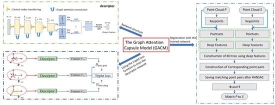
For the irregular characteristics of point cloud, most point cloud processing methods use voxelization or a directly processing model [27]. For the 3D data represented by RGB-D, the representative learnable 3D descriptors extraction networks include 3DMatch [46], PPFNet [30], PPF-FoldNet [31], etc. In the original papers, these methods were tested with indoor data sets, and some of the input [30,31] contained features such as PPF [30,34], instead of the point coordinates. Recently, scholars proposed several new network models to test more types of data. For example, Zhang et al. [47] designed a Siamese network to learn deep feature descriptors for sparse point clouds based on voxel representation, and it was tested with indoor and urban subway tunnel data sets; 3DFeat-Net [29] designed a three-branch Siamese architecture to detect interest points and learn descriptors in a weakly supervised manner. The descriptor extraction module is implemented based on PointNet and has been tested on both indoor and outdoor datasets. Li and Lee [28] proposed an unsupervised learning method (unsupervised stable interest point, USIP), which uses the structure embedding of PointNet in both interests, i.e., point selection and feature extraction. DeepVCP [48] is a registration method, applied to autonomous driving, which directly implements an end-to-end, high-precision registration network on the point cloud. To determine the corresponding points, the PointNet structure is used in the feature embedding layer to obtain a detailed local feature description. In addition to these learnable descriptors, obtained by using a single network type or convolution method, other examples are based on fully convolutional geometric features (FCGF) [49], which adopt the Minkowski convolution to extract the feature of each point. Besides, the perfect match [50] encodes the unstructured 3D point cloud into a smoothed density value (SDV) grid that is convenient for convolving and designing a Siamese CNN to learn the descriptors. The D3Feat [51] uses the kernel point convolution (KPConv) [52] to process irregular point clouds to learn the feature descriptors. There are less abundant studies on the learnable descriptors of fusion features. Here, we list two of the representative works. The first one is the compact geometric features (CGF) [53], in which the hand-crafted descriptors are input into a fully-connected network, with five hidden layers, to obtain learning-based descriptors. Additionally, Yang et al. [54] designed a descriptor of fusion features, obtained by multiple combinations of various hand-designed descriptors with low-level features.

3. Method

The method combined graph attention convolution and 3D capsules into a new neural network model (GACM). The learned, robust, local features of GACM were used to conduct efficient registration for TLS point clouds in the urban scene. The framework of the proposed method is shown in Figure 1. In the training process, we used the farthest point sampling (FPS) algorithm to sample z points in each scan of point cloud as keypoints, and then adopted the k-nearest neighbors (k-NN) algorithm to search k-nearest neighbors of each keypoint in the corresponding point cloud, so that each keypoint corresponds to a point set that is a local point patch, namely P₁, …, P_z. Next, each point set was subsampled by FPS, one-by-one (4 times in total), and combined with graph attention convolution to obtain feature vector of each point in the point set after subsampling. Eventually, a 3D capsule module was added to further extract the features of the point sets, based on these features, to obtain the final deep feature of each point set (dimension size: 32 × 16), through the dynamic routing mechanism. During training, we introduced triplet loss [55] to train the designed network model. The registration process is as follows:

The first step is to generate z keypoints from target point cloud (reference point cloud) and source point cloud (point cloud to be registered) with FPS. The k-NN is then used to obtain the point set corresponding to each keypoint. The point sets are then sent to the trained network to extract the deep feature of each keypoint (the dimension of each extracted deep feature is 32 × 16 corresponding to the point set).

The second step is the construction of KD-tree by using the obtained deep features. The correspondence between keypoints in different point clouds is determined according to the Euclidean distance of deep features of different point sets. The keypoints corresponding to the two pointsets with the smallest Euclidean distance between the features are regarded as an initial matching keypoint pair.

The third step is to use the RANSAC [46] to eliminate the incorrectly matching keypoint pairs from the initial matching keypoint pairs (obtained by the previous step). The keypoint pairs with a distance greater than an empirical threshold (0.5 m in the test of Dataset I and 0.2 m in the test of Dataset II) are eliminated as outliers, and the correctly matched keypoint pairs will be retained in this step.

The fourth step is to calculate the translation matrix (T) and the rotation matrix (R), according to the keypoint pairs, after eliminating the low-quality matching points and registering the source and target point clouds.

3.1. Network Structure

The network structure of feature extraction of point set is depicted in Figure 1 (the green background in the training process). The point set input into the network was k × d dimension (k is the number of points, and d = 3 represents the 3D spatial coordinates of each point). The structure of the proposed GACM includes a graph attention convolution (GAC) module and 3D capsule module (3Dcaps).

3.1.1. Graph Attention Convolution Module

The graph attention convolution module is depicted in the yellow dashed box of the training process of Figure 1. Let the input data before the first GAC operation be a point set P = [p₁, p₂, …, p_k] ∈ R^3×k, which is a local point patch. Each point in the point set only contains 3D spatial coordinates, without any other information. Firstly, we take each point in the point set P as the central node, and a graph G (V, E) is constructed by randomly sampling (n − 1) the neighboring points, within the sphere of radius R for each central node, where V is the node set and E is the set of edges formed by the central node and each neighboring node. If the number of points in the sphere of radius R is less than n, the insufficient parts are randomly sampled from the points in the sphere and replicated. Finally, a centering operation is performed on the spatial coordinates of the n points in each graph G (that is, the coordinates of neighboring points, minus the corresponding coordinates of the center node, respectively), and the centered coordinates are used as the initial features of the n points in the corresponding graph. The GAC is performed, and the details can be found in the next paragraphs. After the r-th central node selection, by using FPS and GAC operations (as shown in the training process of Figure 1, r = 1, 2, 3, and 4, and a total of four times, GAC operations are performed), the point set $P_r=\left[p_{r,1},p_{r,2},\dots ,p_{r,\frac{k}{2^{r-1}}}\right]\in R^{3\times \frac{k}{2^{r-1}}}$ and feature set $F_r=\left[f_{r,1},f_{r,2},\dots ,f_{r,\frac{k}{2^{r-1}}}\right]\in R^{D_r\times \frac{k}{2^{r-1}}}$ ($D_r$ is the dimension of the feature after the r-th GAC operation and $D_r$ = 64 × $2^{r-1}$). The input of the (r + 1)-th center node selection (sampling by FPS) of the GAC operation is matrix $F_r^{\prime }=\left[P_r,F_r\right]\in R^{\left(3+D_r\right)\times \frac{k}{2^{r-1}}}$, which contains the coordinate of each current point and its corresponding features. In the training process of Figure 1, the arrow of central node transferring indicates that the information obtained at the previous level is transferred to the next level. In addition to r = 1, the GAC operation uses the feature passed from the previous layer as the input feature, when r is equal to 2, 3, and 4, respectively.

The specific process of GAC is as follows. Assuming that the current GAC operation is performed for the r-th time, the GAC operation completes the mapping process of the central node feature from $R^{D_{r-1}}$ to $R^{D_r}$. We define S(i) as the point sequence number set of the neighboring point set, formed by the central node i and its neighboring nodes. The schematic diagram of the graph attention convolution of the central node i and its neighbors is shown in Figure 2, where the number of nearest neighboring points is set as n = 32.

In order to complete the mapping process, a shared attention matrix $\alpha \in R^{\left(3+D_r\right)\times D_r}$, is established. Through this learnable variable parameter matrix, the convolution operation can reflect the difference of significance. Particularly, the attention weight ${\widehat{a}}_{ij}$ between the i-th central node and its neighboring points takes into account the position and feature difference of spatial points. The formula is shown as:

$${\widehat{a}}_{ij}=\left(\left[\mathsf{\Delta }{p}_{ij}\oplus \mathsf{\Delta }{f}_{ij}\right]\right)\mathit{\alpha },\hspace{1em}j\in S\left(i\right),$$

(1)

where $\oplus$ represents the concatenate operation, $\mathsf{\Delta }{p}_{ij}=p_{r-1,j}-p_{r-1,i}$, and $\mathsf{\Delta }{f}_{ij}=ML{P}_G\left(f_{r-1,j}\right)-ML{P}_G\left(f_{r-1,i}\right)$.$ML{P}_G\left(·\right)$ is a multi-layer perceptron operation with three layers that maps the feature dimension of each node in the graph structure from $R^{D_{r-1}}$ to $R^{D_r}$. Therefore, ${\widehat{a}}_{ij}=\left[{\widehat{a}}_{ij,1},{\widehat{a}}_{ij,2},\dots ,{\widehat{a}}_{ij,D_r}\right]\in R^{D_r}$, where ${\widehat{a}}_{ij,D_r}$ is the attention weight of the j-th neighboring node to the center node i on the D_r-th channel.

We then normalize all the features on the D_r-th channel, as shown in Equation (2):

$$a_{ij,D_r}=softmax\left({\widehat{a}}_{ij,D_r}\right)=\frac{\exp \left({\widehat{a}}_{ij,D_r}\right)}{{\sum }_{n\in S\left(i\right)}\exp \left({\widehat{a}}_{in,D_r}\right)}$$

(2)

The softmax (·) function is applied to the n-dimensional input tensor and scales it, so that the output element of each n-dimensional input tensor is in the range of [0,1], and all elements sum up as 1.

Finally, the central node i completes the feature update, as shown in Equation (3):

$$f_{r,i}={\displaystyle \sum }_{j\in S\left(i\right)}{a}_{ij}\circ ML{P}_G\left(f_{r-1,j}\right)+b_i,$$

(3)

where the symbol “$\circ$” represents Hadamard product, i.e., the corresponding elements of two matrices are multiplied, and $b_i\in R^{D_r}$ is a learnable offset.

3.1.2. Three-Dimensional Capsule Module

Capsule Network

Sabour et al. [38] and Zhao et al. [33] proved that the capsule network has a great feature extraction capability. Following this inspiration, we introduced a 3D capsule module to further extract features of point clouds in the urban scene. We set up the dynamic routing [38] mechanism in the process of extracting primary point capsules to obtain the final high-level features (as shown in the purple dashed box of Figure 1). We set $u_i$ as the output vector of the capsule i in the primary point capsules, $w_{ij}$ as the affine transformation matrix from the capsule i to its higher-level of capsule j, and the input prediction vector is expressed as ${\widehat{u}}_{j|i}=w_{ij}{u}_i$. The algorithm process (namely Algorithm 1) of the dynamic routing is as follows:

Algorithm 1: Dynamic routing algorithm.

1: Input: The prediction vector ${\widehat{u}}_{j|i}$, iteration number t.

2: Output: Deep capsule vector $v_j$.

3: For every capsule i in the primary point capsule layer and capsule j in the output feature layer:   Initialize the logits of coupling coefficients $b_{j|i}$= 0.

4: For t iterations do

5: For every capsule i in the primary point capsule layer: $c_{j|i}=softmax\left(b_{j|i}\right)=\frac{\exp \left(b_{j|i}\right)}{{\sum }_k\exp \left(b_{k|i}\right)}$.

6: For every capsule j in the output feature layer: $v_j=squash\left({\sum }_i{c}_{j|i}{\widehat{u}}_{j|i}\right).$

7: For every capsule i in the primary point capsule layer and the capsule j in the output feature layer: $b_{j|i}=b_{j|i}+{\widehat{u}}_{j|i}·v_j$.

8: Return $v_j$

In the above algorithm, the squash (·) function is defined as:

$$squash\left(x\right)=\frac{{\parallel x\parallel }^2}{1+{\parallel x\parallel }^2}\frac{x}{\parallel x\parallel }.$$

(4)

The nonlinear function squash (·) completes the compression of the vector, so that the length of the output vector can represent the probability of the entity.

The Specific Operation in 3D Capsule Module

The 3D capsule module is shown in the purple dotted box of Figure 1. In this module, we used the output $F_{\mathrm{GAC}}^{512\times \frac{k}{8}}$ of the graph attention convolution module as the input of 3D capsule module. Specifically, the feature dimension of $\frac{k}{8}$ points, processed by the graph attention convolution, were converted from 512 to 1024 through a fully-connected layer (e.g., the FC in the purple dotted box of Figure 1), and the converted feature matrix ($F^{1024\times \frac{k}{8}}$) was mapped to multiple independent convolutional layers with different weights (we designed 16 independent convolutional layers in the experiments). The max pooling was used to obtain global features in each independent convolutional layer. Next, the global features in the 16 independent convolutional layers were concatenated into primary point capsules (the size of the primary point capsules we used in the experiments was 1024 × 16). Finally, the primary point capsules generated a high-level feature, with a dimension of 32 × 16, through the dynamic routing mechanism, and we took the high-level feature as the final constructed deep feature.

3.2. Training Process

3.2.1. Loss Function

The training process is shown in Figure 3. We used the triplet loss [55] as the loss function to train the model. During the training process, this function reduces the distance between the features of matching points and enlarges the distance between the features of non-matching points. Through this optimization function, more prominent features of urban point clouds can be obtained.

We defined the anchor point set and the positive point set as P_anc and P_pos, respectively. They form the matching point pairs in the two sets of points. Similarly, the anchor point set P_anc and the negative point set P_neg are defined as the non-matching point pairs. The generation processes of P_anc, P_pos, and P_neg will be described in the next section (namely “Section 3.2.2 The construction of training point pairs”). The triplet loss is calculated according to formula (5):

$$L_T=\max \left(D_{anc,pos}-D_{anc,neg}+M,0\right),$$

(5)

where D_anc,pos/D_anc,neg represents the Euclidean distance between the features of matching/non-matching point pairs, and M stands for the margin value between the positive and negative pairs.

3.2.2. The Construction of Training Point Pairs

The point cloud of each scan, in the urban scene, in the following operation is in the global coordinate system, which can be used as the true value of registration. In the training stage, we first used FPS to obtain interest points in the training scene (we set the scan number as τ), and the obtained interest points were set as keypoints to form a set of keypoints $P^{\tau }=\left\{p_1^{\tau },p_2^{\tau },\dots ,p_z^{\tau }\right\}$. $p_i^{\tau }$ was the i-th keypoint in the scan #τ, where $i=\left\{1,2,\dots ,z\right\}$. Then, in the two adjacent scans, i.e., scan #(τ + 1) and scan #(τ + 2), we queried whether there were corresponding keypoints, whose Euclidean distance from $p_i^{\tau }$ was less than the threshold (0.05 m in the experiments). If there are multiple points, the nearest point was selected as the corresponding point; if it did not exist, the point in $P^{\tau }$ was removed. After the above process, the point set $P_{\tau }^{\tau ,\tau +1}=\left\{p_1^{\tau ,\tau +1},p_2^{\tau ,\tau +1},\dots ,p_q^{\tau ,\tau +1}\right\}$ represents the final set of keypoints of the scan #τ, and $P_{\tau +1}^{\tau ,\tau +1}=\left\{p_1^{\tau ,\tau +1},p_2^{\tau ,\tau +1},\dots ,p_{q\prime }^{\tau ,\tau +1}\right\}$ represents the final set of keypoints of the scan #(τ + 1). In other words, the points in the point set $P_{\tau }^{\tau ,\tau +1}$ and $P_{\tau +1}^{\tau ,\tau +1}$ correspond one-to-one, thus becoming a pair of corresponding points. Taking $P_{\tau }^{\tau ,\tau +1}$ as the anchor point set $P_{anc}^{\tau ,\tau +1}$, we rotated the point set $P_{\tau +1}^{\tau ,\tau +1}$ randomly from 0 to 360 degrees and translated them randomly from 0 to 100 m as the positive point set $P_{pos}^{\tau ,\tau +1}$. The points in $P_{pos}^{\tau ,\tau +1}$ were swapped, in random order, as the negative point set $P_{neg}^{\tau ,\tau +1}$. Similarly, the scan #τ and #(τ + 2) could also construct the anchor $P_{anc}^{\tau ,\tau +2}$, positive $P_{pos}^{\tau ,\tau +2}$, and negative point sets $P_{neg}^{\tau ,\tau +2}$. In the same way, we use the anchor, the positive, and the negative point sets for different scans (such as scan #0, #1, …, #19) to complete the construction of the training set.

During the training process, for each keypoint in the anchor, positive, and negative point sets, its k-nearest neighboring points in the corresponding scan are searched through the k-NN algorithm, where a point set (a local point patch) is constructed as the input of the proposed network. Finally, we obtain the deep features corresponding to each point in the anchor, positive, and negative point sets, and use triplet loss to optimize the model.

3.3. Point Cloud Registration

We used the trained model to test the registration results of TLS point clouds in the urban scene. Firstly, we used the FPS to obtain z interest points, namely the keypoints in each scan. Secondly, we search the k-nearest neighbors for each interest point in the respective scan. The corresponding point sets of z interest points are formed, respectively. Thirdly, the z point sets were used as input for the trained network model. For each point set, four consecutive graph attention convolution operations were performed to update and obtain the features of nodes in the point set (the dimension of the features in each point set is $\frac{k}{8}\times 512$). After that, with the help of capsule network we proposed, the features of point set were inserted into independent convolutional layers, under different weights, to produce their global features. The global features in different independent convolutional layers were used to construct primary point capsules. Finally, high-level features were obtained through the dynamic routing. Each high-level feature corresponded to each keypoint.

After each keypoint feature extraction was completed, the extracted feature corresponding to each keypoint was used to construct KD-tree. If the Euclidean distance of the features of two keypoints in the two-point clouds is shortest, we regarded the two keypoints as a matching point pair. Then the RANSAC algorithm was used to eliminate mismatched point pairs. In this process, the point pairs with a feature distance below the threshold (0.5 m in the experiments) were saved as inliers, and the point pairs with a feature distance above the threshold were eliminated as outliers. Inliers were used to calculate the rotation matrix R and translation matrix T by singular value decomposition, in order to further realize the registration of two scans of point clouds in the urban scene.

4. Experiments and Results

First, we performed a sensitivity analysis of the model parameters and compared our method with the other four methods of point cloud registration, in order to deeply analyze the performance of our method. The implementation details of our model include: Pytorch 1.1.0 and NVIDIA GeForce RTX 2080Ti. In the training phase, we used the Adam optimizer, where the learning rate is set to 0.0001. The margin in triplet loss (namely the M in Equation (5)) is set to 0.2. The training samples include a set of 19,000 pairs of point sets. The batch size is 15, and the epoch number 100.

4.1. Datasets

We used four datasets (Datasets I-IV) for the experiments, all of which come from the ETH open datasets [56]. Datasets I-IV are ETH Hauptgebaude, Stairs, Apartment and Gazebo (winter), respectively. The specific information of the four datasets is shown in

Table 1. Properties of the four datasets.

Dataset	Dataset I (ETH Hauptgebaude)	Dataset II (Stairs)	Dataset III (Apartment)	Dataset IV (Gazebo (Winter))
Situation	Indoors	Indoors/Outdoors	Indoors	Outdoors
Number of scan	36	31	45	32
Mean points/scan	191,000	191,000	365,000	153,000
Scene size	62 m × 65 m × 18 m	21 m × 111 m × 27 m	17 m × 10 m × 3 m	72 m × 70 m × 19 m

. These four datasets provide TLS point clouds in base frame (the point clouds coordinate origin is at the center of the scanner) and TLS point clouds in global frame (the point clouds are moved to a global reference coordinate system). During point cloud registration, scans #0 to #19 of Dataset I were used for training, and scans #20 to #35 of Dataset I test the registration results of TLS point clouds. Since there were certain overlapping areas of adjacent scans in the test scene, the scan #(t + 1) in base frame is registered to the scan #t in global frame during the registration test of Dataset I (20 ≤ t ≤ 35 and t$\in N$, and a total of 15 pairs of registrations are completed). Similarly, there were 31 scans in Dataset II, and the scan #(t + 1) in base frame is registered to the scans #t in global frame to complete the registration test of Dataset II (0 ≤ t ≤ 30 and t$\in N$, and a total of 30 pairs of registrations are completed). For Dataset III and Dataset IV, we only performed three deep learning methods to register scan #1 to scan #0.

4.2. Parameter Sensitivity Analysis

We performed registration tests on the 15 scans of Dataset I, which were not used during the training of Dataset I, to explore the impacts of keypoint number (z) and the point number of each point set (k) on the registration accuracy of our method. We set z to 3000, 5000, 8000, and k to 128, 256, and 512, respectively. The root mean squared errors (RMSEs) of registration under different values of z and k are shown in Figure 4. RMSE is the error value of all points in the scan. We can see that, with the increasing of k value, the RMSE value becomes smaller in general. In terms of the mean and standard deviation, the worse RMSE value of registration in Figure 4 is obtained when k = 128 and z = 3000, and better registration results are obtained when k = 512 and z = 3000. To fully test the performance of our method, in the following experiments, we use k = 128 and z = 3000 and k = 512 and z = 3000 to compare with other methods.

4.3. Comparison with Other Methods

In order to verify the performance of our method, we compared the registration results with the other four methods in Datasets I-II. The first method (Method I) was Super4PCS [19], which is a variant of 4PCS and mainly uses an affine invariance of four coplanar points for global registration of point clouds. The second method (Method II) was fast global registration [17], which uses FPFH to determine the correspondence between points. The third method (Method III) was 3DFeat-Net [29], which constructs deep features under a weakly supervised way to perform point cloud registration. The fourth method (Method IV) [47] designs a voxel-based 3D convolutional neural network to construct 3D deep features of point clouds. Methods III and IV belong to deep learning framework.

We refer to the evaluation indicators [57], namely relative rotational error (RRE) and relative translational error (RTE), to evaluate the effects of registration. RRE is calculated as follows:

$$\begin{gathered} \mathrm{RRE}={\sum }_{i=1}^3\left|angl{e}_i\right|, \\ angle=F\left(R_T^{-1}{R}_E\right), \end{gathered}$$

(6)

where F(·) transforms a rotation matrix to three Euler angles, R_T is the ground-truth rotation matrix, and R_E is the estimated rotation matrix. RRE is the sum of the absolute differences of the three Euler angles.

RTE is calculated as follows:

$$\mathrm{RTE}={∥T_T-T_E∥}_2,$$

(7)

where T_T is the ground-truth translation vector and T_E is the estimated translation vector.

4.3.1. Test Results on Dataset I

In Dataset I, each method performs 15 pairs of adjacent scans.

Table 2. The registration success rates of different methods in Dataset I.

Method	Success Rate	Success Rate	Success Rate
	(RTE < 1 m and RRE ≤ 10°)	(RTE < 1 m and RRE ≤ 5°)	(RTE < 0.5 m and RRE ≤ 2.5°)
Method I	10/15 (67%)	8/15 (53%)	4/15 (27%)
Method II	11/15 (73%)	4/15 (27%)	0/15 (0%)
Method III	15/15 (100%)	15/15 (100%)	5/15 (33%)
Method IV	15/15 (100%)	13/15 (87%)	4/15 (27%)
Our method (k = 128)	15/15 (100%)	15/15 (100%)	6/15 (40%)
Our method (k = 512)	15/15 (100%)	15/15 (100%)	9/15 (60%)

shows the registration results of the 15 pairs of registration. The values of RRE and RTE are errors for all points in scans.

Besides, we set three standards for a successful registration: RTE < 1 m and RRE ≤ 10°, RTE < 1 m and RRE ≤ 5°, and RTE < 0.5 m and RRE ≤ 2.5°. During the experiments, the keypoint number (z) for both our method and Method IV are set to 3000. As shown in Table 2, our method achieves the highest successful registration rate under the three standards.

A pair of registration results is randomly selected for visual comparison (e.g., scan #34 and scan #33). As shown in

Table 3. Registration results of each method from scan #34 to scan #33 in Dataset I.

Method	RTE (m)	RRE (°)
Method I	0.41	3.4
Method II	0.59	11.0
Method III	0.83	2.8
Method IV	0.32	5.4
Our method (k = 128)	0.40	1.8
Our method (k = 512)	0.05	1.0

and Figure 5, the visual results of our method are better than Methods I-IV, which further illustrate the capability of the proposed GACM.

To further compare the performance of extracting rotation invariant feature in three deep learning-based methods (namely Methods III-IV and our method), we rotate each point cloud to be registered in 15 pairs of point clouds by 30° and 60° around z-axis, respectively. The registration success rates of the three deep learning-based methods are shown in

Table 4. Registration results of each method from scan #34 to scan #33 in Dataset I.

Method	Success Rate (RTE < 1 m and RRE ≤ 10°)
	30°	60°
Method III	13/15 (87%)	12/15 (80%)
Method IV	10/15 (67%)	0/15 (0%)
Our method (k = 512)	15/15 (100%)	13/15 (87%)

. It shows that the registration success rates of Methods III-IV decreased after the point cloud to be registered is rotated by 30° or 60°, while our method still maintains a robust performance, verifying the capability of anti-rotation in GACM.

4.3.2. Test Results on Dataset II

During training, each of the learning-based methods (e.g., Methods III, IV, and our method) does not use Dataset II (namely the Stairs). To verify the generalization capability of our method, we test the model in Dataset II only using the parameters learned from Dataset I and compared it with the other four methods. Unlike Dataset I, many adjacent scans of point clouds in Dataset II change greatly, and the initial orientation difference is also large. Figure 6 also show that the point density in many local areas are extremely low, making it even more challenging for registration. To adequately extract long-range contextual information of point clouds in the urban scene, we use k-NN algorithm to construct neighborhood in point clouds to ensure robust expression of the region (described in the part of “3. Method”). The registration starts from scan #1 to scan #0, and the registrations of 30 pairs of adjacent scans are completed. The keypoint number z for both our method and Method IV are set to 3000. As shown in

Table 5. The registration success rate of each method in Dataset II.

Method	Success Rate	Success Rate	Success Rate
	(RTE < 1 m and RRE ≤ 10°)	(RTE < 1 m and RRE ≤ 5°)	(RTE < 0.5 m and RRE ≤ 2.5°)
Method I	23/30 (77%)	14/30 (47%)	3/30 (10%)
Method II	11/30 (37%)	9/30 (30%)	2/30 (7%)
Method III	9/30 (30%)	7/30 (23%)	2/30 (7%)
Method IV	8/30 (27%)	1/30 (3%)	1/30 (3%)
Our method (k = 128)	27/30 (90%)	24/30 (80%)	17/30 (57%)
Our method (k = 512)	28/30 (93%)	24/30 (80%)	18/30 (60%)

, under the three successful registration standards, our method achieves higher registration success rates when k = 128 and k = 512 than the compared methods. Using our method with k = 512 can obtain higher success rates than that of k = 128. The success rate of the Method I in Dataset II is about 70% under the laxest constraint (RTE < 1 m and RRE ≤ 10°), and the success rate decreases sharply when the constraint condition becomes severe (e.g., RTE < 1 m and RRE ≤ 5° and RTE < 0.5 m and RRE ≤ 2.5°). The success rate of Method II in Dataset II is significantly lower than that in the Dataset I, which is consistent with the fact that the Dataset II is more complex and the overlap between adjacent scans is less than Dataset I. The performance of deep learning method (Methods III and IV) in the Dataset II is worse than that in the Dataset I, which reflects the limitation of generalization.

The registration results of a pair of scans are randomly selected for visualization (e.g., the scan #25 is registered to the scan #24), as shown in Figure 6. Figure 6a shows some points of the two unregistered scans are far away from the main part (highlighted in the yellow boxes), and the registration results of each method are shown in Figure 6b–f, with enlarged displays of the main part. As shown in

Table 6. Registration results of each method from scan #25 to scan #24 in Dataset IIr.

Method	RTE (m)	RRE (°)
Method I	0.50	13.1
Method II	0.33	37.1
Method III	2.09	53.5
Method IV	4.45	178.6
Our method (k = 128)	0.23	1.9
Our method (k = 512)	0.10	2.5

, our method achieves successful registration under the strictest standard (RTE < 0.5 m and RRE ≤ 2.5°), when k = 128 and k = 512, and the other four methods do not reach the laxest standard (RTE < 1 m and RRE ≤ 10°). The effect of orientation difference to the registration of the compared methods is large, especially Method IV, which has a serious direction error, and RRE is close to 180°.

In further analysis, we found that each compared method almost fails in the registration of some pairs of scans. As shown in

Table 7. The scans where the registrations of most comparison methods fail by using Dataset II under the registration success standard (RTE < 1 m and RRE ≤ 10°).

Scans		Method
		I	II	III	IV	Our Method (k = 128)	Our Method (k = 512)
#1 to #0	RTE (m)	0.20	0.41	0.91	0.38	0.13	0.02
	RRE (°)	4.5	11.3	18.1	12.3	1.8	1.2
#5 to #4	RTE (m)	2.20	0.42	0.22	1.90	0.27	0.17
	RRE (°)	7.2	9.6	10.6	76.4	2.0	3.6
#15 to #14	RTE (m)	0.38	0.45	0.28	0.38	0.11	0.3
	RRE (°)	8.7	16.3	14.6	12.1	2.7	10.9
#25 to #24	RTE (m)	0.50	0.33	2.09	4.45	0.23	0.1
	RRE (°)	13.1	37.1	53.5	178.6	1.9	2.5
#26 to #25	RTE (m)	1.25	0.3	0.45	3.05	0.52	0.15
	RRE (°)	19	29.4	4.1	222.3	22.7	3.2
#27 to #26	RTE (m)	1.50	0.34	1.36	2.92	0.69	0.27
	RRE (°)	8.3	9.4	17.5	268.0	2.0	2.0

, among 30 pairs of registrations, we chose 6 pairs of scans, in which the registrations of most comparison methods failed under the laxest registration success standard (RTE < 1 m and RRE ≤ 10°), and our method basically maintained the optimal RTE and RRE in the corresponding registration. In the registration from scan #15 to scan #14, our method failed when k = 512, but its RRE value was close to the registration requirement (RRE ≤ 10°). Compared with the other two deep learning registration methods (Methods III and IV), our method can fix the effects of initial orientation differences and remains relatively stable, which illustrates the ability of extracting the rotation-invariant feature in the proposed GACM.

4.3.3. Test Results on Dataset III and Dataset IV

Our method, and the two contrasting deep learning methods (Methods III-IV), are not trained on Datasets III-IV. Here, our goal was to further test the robustness of each deep learning method, in different urban scene environments, after only training in the Dataset I. As shown in Figure 7, the initial position rotation deviation of Datasets III-IV was small, but the density of Dataset III or geometric shape of Dataset IV was quite different from the training set (Dataset I). Figure 7e shows that the scanning on the ground seriously interferes with the visual result. We filter out the ground, that is, Figure 7f,g shows the registration results of each method after removing the ground points. By observing the red marked boxes in Figure 7, the registration results of Methods III-IV still have large translation deviations, and our results are better than them.

4.4. Ablation Experiments

In order to further study the performance of the proposed GACM, we conducted the ablation experiments. In

Table 8. Contrastive analysis of descriptor extraction networks in Dataset II.

Network Structure	Success Rate (RTE < 1 m and RRE ≤ 10°)	Success Rate (RTE < 1 m and RRE ≤ 5°)	Success Rate (RTE < 0.5 m and RRE ≤ 2.5°)
GAC	25/30 (83%)	24/30 (80%)	16/30 (53%)
3DCaps	0/30 (0%)	0/30 (0%)	0/30 (0%)
GAC + 3DCaps (ours)	27/30 (90%)	24/30 (80%)	17/30 (57%)

, the GAC represents the graph attention convolution module, and 3DCaps represents the 3D capsule module. When using the GAC alone (corresponding to the yellow dotted box in Figure 1), we added the max-pooling to obtain the 512-dimensional features as the output. When using the 3DCaps alone (corresponding to the purple dotted box in Figure 1), MLP (multi-layer perceptron) was used to complete 128-dimensional generation, according to the encoder section of 3D point capsule networks [33]. In the experiments, except for the above difference in network structure, all other hardware and software conditions were the same. The number of keypoints in the GAC and GAC+3DCaps were both z = 3000 and k = 128. The results showed that the network structure of our method (GAC+3Dcaps, namely GACM) tends to have a higher registration success rate under various conditions than using the GAC network structure alone. When the input is coordinates alone and the number of training sets is not greatly expanded, 3DCaps cannot be used for registration. It proves that the proposed GACM is beneficial to the registration results.

In the experiments, we found that the unsuccessful registration of each method often occurs when the RRE exceeds the constraint condition and mainly occurred in the registration of the last six pairs of scans. To further understand the effects of the 3DCaps module, we compared and analyzed the RRE values of the two network structures (GAC and GAC+3DCaps) in the registration of the last six pairs of scans in Dataset II. RRE of the registration results are shown in

Table 9. The RRE (°) of registration results of GAC and GAC+ 3DCaps (our method) in the last six pairs of scans of Dataset II.

Registration Scans	GAC (z = 3000 and k = 128)	GAC + 3DCaps (Our Method with z = 3000 and k = 128)
#25 to #24	43.2	1.9
#26 to #25	21.6	22.7
#27 to #26	11.5	2.0
#28 to #27	42.3	15.9
#29 to #28	4.0	3.8
#30 to #29	24.7	12.3

. We see that the rotation errors of the registration are reduced with the GAC+3DCaps structure (namely GACM), which is especially true for the scans where the registration fails when only using GAC. We conclude that the descriptors obtained by combining GAC and 3DCaps (namely GACM) are more effective than the descriptors obtained by only using the GAC.

5. Discussion

The four comparison methods include two traditional methods and two deep learning methods. Table 3 and Table 5 show that, during the training stage for Dataset I, the deep learning methods have a higher registration success rate than the traditional methods (as shown in Table 2). The performance of the two compared deep learning methods are not as advantageous as the traditional ones when scene difference between training data and test data is large. So, the compared network model (e.g., Methods III and IV) is limited, while our method can maintain a robust performance in the case of large scene difference. After reducing the scene difference (e.g., the experiments in Table 2), the registration results of two compared methods (e.g., Methods III and IV) are not better than our method.

In the test of Section 4.2, the numbers of keypoint z between 3000–8000 have less effects on RMSE. It may be caused by the RANSAC threshold (in the third step of Figure 1) set by us. If the threshold is set to 0.1 m and z is 3000, the keypoints in some local region of a pair of registered point clouds may not have corresponding points. On the other hand, if z is set to 8000, these parts may have corresponding key points within the threshold of 0.1 m. For the range from z = 3000 to z = 8000, with the threshold of 0.5 m, there are always corresponding key points within 0.5 m.

During the test of Dataset II, our methods, as well as the four comparison methods, all have large errors in the last six scans. We believe that it is affected by the following factors: (1) the six scans are all similar to the situation in Figure 6a, except that the initial rotation deviation is large, and some noise points are still far away from the main body. (2) Small clusters on these surfaces (for example, the yellow box in Figure 6a) cannot provide an effective geometric shape. (3) The overall density distributions of these scans are extremely uneven.

6. Conclusions

This research proposes a new network model (namely GACM) to extract the 3D feature descriptors of TLS point clouds in the urban scene. The GACM combines graph attention convolution and a 3D capsule network to obtain a discriminative, anti-rotation descriptor that can represent the feature of complex urban scene and be utilized to realize the high-quality registration. The experimental results on the four public datasets prove that our method has higher pairwise registration performance than other four frontier methods, without augmenting a heavy training, especially for the point clouds with relatively large orientation and angle differences. We also achieve the highest registration success rates in different standards. In the strictest standard (RTE < 0.5 m and RRE ≤ 2.5°), our registration success rates are 30% higher than the four comparison methods on the test datasets. Although our method performs better than the other two deep learning-based methods in untrained data set tests, it cannot complete a successful registration (RTE < 1 m and RRE ≤ 10°) of all scan tests, as in trained data set tests. In our method, furthest point sampling is adopted to obtain keypoints, in order to ensure that the spatial distribution of keypoints is relatively uniform. However, when the overlap region of two set of point clouds is very small, the calculation of the descriptors of the non-overlapping regions is invalid and unnecessary, which has not been solved by us.

In the future, we will explore the automatic determination of the overlapping area between the target point clouds and source point clouds to reduce the calculation of descriptors to obtain a better registration effect.

References

1. Jelalian, A.V. Laser Radar Systems; Artech House: Boston, MA, USA; London, UK, 1992. [Google Scholar]
2. Urech, P.R.; Dissegna, M.A.; Girot, C.; Grêt-Regamey, A. Point cloud modeling as a bridge between landscape design and planning. Landsc. Urban Plan. 2020, 203, 103903. [Google Scholar] [CrossRef]
3. Chen, X.; Ma, H.; Wan, J.; Li, B.; Xia, T. In Multi-view 3d object detection network for autonomous driving. In Proceedings of the IEEE Conference on Computer Vision and Pattern Recognition, Honolulu, HI, USA, 21–26 July 2017; pp. 1907–1915. [Google Scholar]
4. Nilsson, M.; Nordkvist, K.; Jonzén, J.; Lindgren, N.; Axensten, P.; Wallerman, J.; Egberth, M.; Larsson, S.; Nilsson, L.; Eriksson, J. A nationwide forest attribute map of Sweden predicted using airborne laser scanning data and field data from the National Forest Inventory. Remote Sens. Environ. 2017, 194, 447–454. [Google Scholar] [CrossRef]
5. Badenko, V.; Zotov, D.; Muromtseva, N.; Volkova, Y.; Chernov, P. Comparison of software for airborne laser scanning data processing in smart city applications. Int. Arch. Photogram. Remote Sens. Spat. Inform. Sci. 2019, XLII-5/W2, 9–13. [Google Scholar] [CrossRef] [Green Version]
6. Endres, F.; Hess, J.; Sturm, J.; Cremers, D.; Burgard, W. 3-D mapping with an RGB-D camera. IEEE Trans. Robot. 2014, 30, 177–187. [Google Scholar] [CrossRef]
7. Li, L.; Liu, Y.H.; Wang, K.; Fang, M. Estimating position of mobile robots from omnidirectional vision using an adaptive algorithm. IEEE Trans. Cybern. 2017, 45, 1633–1646. [Google Scholar] [CrossRef]
8. Liu, M. Robotic online path planning on point cloud. IEEE Trans. Cybern. 2016, 46, 1217–1228. [Google Scholar] [CrossRef]
9. Vosselman, G.; Dijkman, S. 3D building model reconstruction from point clouds and ground plans. Int. Arch. Photogramm. Remote Sens. Spat. Inform. Sci. 2001, XXXIV-3/W4, 37–44. [Google Scholar] [CrossRef] [Green Version]
10. Wang, F.; Zhuang, Y.; Zhang, H.; Gu, H. Real-time 3-D semantic scene parsing with LiDAR sensors. IEEE Trans. Cybern. 2020, 1–13. [Google Scholar] [CrossRef]
11. Parmehr, E.G.; Fraser, C.S.; Zhang, C.; Leach, J. Automatic registration of optical imagery with 3D LiDAR data using statistical similarity. ISPRS J. Photogramm. Remote Sens. 2014, 88, 28–40. [Google Scholar] [CrossRef]
12. Xu, Z.; Xu, E.; Zhang, Z.; Wu, L. Multiscale sparse features embedded 4-points congruent sets for global registration of TLS point clouds. IEEE Geosci. Remote Sens. Lett. 2018, 16, 286–290. [Google Scholar] [CrossRef]
13. Besl, P.J.; McKay, N.D. Method for registration of 3-D shapes. IEEE Trans. Pattern Anal. Mach. Intell. 1992, 14, 239–256. [Google Scholar] [CrossRef]
14. Bae, K.-H.; Lichti, D.D. A method for automated registration of unorganised point clouds. ISPRS J. Photogramm. Remote Sens. 2008, 63, 36–54. [Google Scholar] [CrossRef]
15. Gressin, A.; Mallet, C.; Demantké, J.; David, N. Towards 3D lidar point cloud registration improvement using optimal neighborhood knowledge. ISPRS J. Photogramm. Remote Sens. 2013, 79, 240–251. [Google Scholar] [CrossRef] [Green Version]
16. Aiger, D.; Mitra, N.J.; Cohen-Or, D. 4-points congruent sets for robust pairwise surface registration. ACM Trans. Graph. 2008, 27, 1–10. [Google Scholar] [CrossRef] [Green Version]
17. Zhou, Q.Y.; Park, J.; Koltun, V. Fast global registration. In Proceedings of the 14th European Conference on Computer Vision, Amsterdam, The Netherlands, 8–16 October 2016; pp. 766–782. [Google Scholar]
18. Rusu, R.B.; Blodow, N.; Marton, Z.C.; Beetz, M. Aligning point cloud views using persistent feature histograms. In Proceedings of the 2008 IEEE/RSJ International Conference on Intelligent Robots and Systems, Nice, France, 22–26 September 2008; pp. 3384–3391. [Google Scholar]
19. Mellado, N.; Aiger, D.; Mitra, N.J. Super 4pcs fast global pointcloud registration via smart indexing. Comput. Graph. Forum 2014, 33, 205–215. [Google Scholar] [CrossRef] [Green Version]
20. Eggert, D.W.; Lorusso, A.; Fisher, R.B. Estimating 3-D rigid body transformations: A comparison of four major algorithms. Mach. Vis. Appl. 1997, 9, 272–290. [Google Scholar] [CrossRef]
21. Rusu, R.B.; Blodow, N.; Beetz, M. Fast point feature histograms (FPFH) for 3D registration. In Proceedings of the 2009 IEEE International Conference on Robotics and Automation, Kobe, Japan, 12–17 May 2009; pp. 3212–3217. [Google Scholar]
22. Cheng, L.; Chen, S.; Liu, X.; Xu, H.; Wu, Y.; Li, M.; Chen, Y. Registration of laser scanning point clouds: A review. Sensors 2018, 18, 1641. [Google Scholar] [CrossRef] [Green Version]
23. Ge, X.; Hu, H. Object-based incremental registration of terrestrial point clouds in an urban environment. ISPRS J. Photogramm. Remote Sens. 2020, 161, 218–232. [Google Scholar] [CrossRef]
24. Wu, Z.; Song, S.; Khosla, A.; Yu, F.; Zhang, L.; Tang, X.; Xiao, J. 3d shapenets: A deep representation for volumetric shapes. In Proceedings of the IEEE Conference on Computer Vision and Pattern Recognition, Boston, MA, USA, 7–12 June 2015; pp. 1912–1920. [Google Scholar]
25. Ku, J.; Mozifian, M.; Lee, J.; Harakeh, A.; Waslander, S.L. Joint 3d proposal generation and object detection from view aggregation. In Proceedings of the 2018 IEEE/RSJ International Conference on Intelligent Robots and Systems, Madrid, Spain, 1–5 October 2018; pp. 1–8. [Google Scholar]
26. Li, L.; Zhu, S.; Fu, H.; Tan, P.; Tai, C.L. End-to-end learning local multi-view descriptors for 3D point clouds. In Proceedings of the IEEE Conference on Computer Vision and Pattern Recognition, 14–19 June 2020; pp. 1919–1928. [Google Scholar]
27. Qi, C.R.; Su, H.; Mo, K.; Guibas, L.J. Pointnet: Deep learning on point sets for 3d classification and segmentation. In Proceedings of the IEEE Conference on Computer Vision and Pattern Recognition, Honolulu, HI, USA, 21–26 July 2017; pp. 652–660. [Google Scholar]
28. Li, J.; Lee, G.H. Usip: Unsupervised stable interest point detection from 3d point clouds. In Proceedings of the IEEE/CVF International Conference on Computer Vision, Seoul, Korea, 27–28 October 2019; pp. 361–370. [Google Scholar]
29. Yew, Z.J.; Lee, G.H. 3dfeat-net: Weakly supervised local 3d features for point cloud registration. In Proceedings of the European Conference on Computer Vision (ECCV), Munich, Germany, 8–14 September 2018; pp. 607–623. [Google Scholar]
30. Deng, H.; Birdal, T.; Ilic, S. Ppfnet: Global context aware local features for robust 3d point matching. In Proceedings of the IEEE Conference on Computer Vision and Pattern Recognition, Salt Lake City, UT, USA, 18–22 June 2018; pp. 195–205. [Google Scholar]
31. Deng, H.; Birdal, T.; Ilic, S. Ppf-foldnet: Unsupervised learning of rotation invariant 3d local descriptors. In Proceedings of the European Conference on Computer Vision (ECCV), Munich, Germany, 8–14 September 2018; pp. 602–618. [Google Scholar]
32. Yew, Z.J.; Lee, G.H. Rpm-net: Robust point matching using learned features. In Proceedings of the IEEE Conference on Computer Vision and Pattern Recognition, Seattle, WA, USA, 14–19 June 2020; pp. 11824–11833. [Google Scholar]
33. Zhao, Y.; Birdal, T.; Deng, H.; Tombari, F. 3D point capsule networks. In Proceedings of the IEEE Conference on Computer Vision and Pattern Recognition, Long Beach, CA, USA, 16–20 June 2019; pp. 1009–1018. [Google Scholar]
34. Birdal, T.; Ilic, S. Point pair features based object detection and pose estimation revisited. In Proceedings of the 2015 International Conference on 3D Vision (3DV), Lyon, France, 19–22 October 2015; pp. 527–535. [Google Scholar]
35. Kipf, T.N.; Welling, M. Semi-supervised classification with graph convolutional networks. arXiv 2016, arXiv:1609.02907. [Google Scholar]
36. Li, G.; Muller, M.; Thabet, A.; Ghanem, B. Deepgcns: Can gcns go as deep as cnns? In Proceedings of the IEEE/CVF International Conference on Computer Vision, Seoul, Korea, 27–28 October 2019; pp. 9267–9276. [Google Scholar]
37. Wang, Y.; Sun, Y.; Liu, Z.; Sarma, S.E.; Bronstein, M.M.; Solomon, J.M. Dynamic graph cnn for learning on point clouds. ACM Trans. Graph. 2019, 38, 1–12. [Google Scholar] [CrossRef] [Green Version]
38. Sabour, S.; Frosst, N.; Hinton, G.E. Dynamic routing between capsules. In Proceedings of the 31st Annual Conference on Neural Information Processing Systems, Long Beach, CA, USA, 4–9 December 2017; pp. 3856–3866. [Google Scholar]
39. Johnson, A.E.; Hebert, M. Using spin images for efficient object recognition in cluttered 3D scenes. IEEE Trans. Pattern Anal. Mach. Intell. 1999, 21, 433–449. [Google Scholar] [CrossRef] [Green Version]
40. Belongie, S.; Malik, J.; Puzicha, J. Shape matching and object recognition using shape contexts. IEEE Trans. Pattern Anal. Mach. Intell. 2002, 24, 509–522. [Google Scholar] [CrossRef] [Green Version]
41. Frome, A.; Huber, D.; Kolluri, R.; Bülow, T.; Malik, J. Recognizing objects in range data using regional point descriptors. In Proceedings of the 8th European Conference on Computer Vision, Prague, Czech Republic, 11–14 May 2004; pp. 224–237. [Google Scholar]
42. Tombari, F.; Salti, S.; Di Stefano, L. Unique shape context for 3D data description. In Proceedings of the ACM Workshop on 3D Object Retrieval, Firenze, Italy, 25 October 2010; pp. 57–62. [Google Scholar]
43. Guo, Y.; Sohel, F.A.; Bennamoun, M.; Wan, J.; Lu, M. RoPS: A local feature descriptor for 3D rigid objects based on rotational projection statistics. In Proceedings of the 2013 1st International Conference on Communications, Signal Processing, and Their Applications (ICCSPA), Sharjah, United Arab Emirates, 12–14 February 2013; pp. 1–6. [Google Scholar]
44. Salti, S.; Tombari, F.; Di Stefano, L. SHOT: Unique signatures of histograms for surface and texture description. Comput. Vis. Image Underst. 2014, 125, 251–264. [Google Scholar] [CrossRef]
45. Steder, B.; Rusu, R.B.; Konolige, K.; Burgard, W. NARF: 3D range image features for object recognition. In Proceedings of the Workshop on Defining and Solving Realistic Perception Problems in Personal Robotics at the IEEE/RSJ International Conference on Intelligent Robots and Systems (IROS), Taipei, Taiwan, 18–22 October 2010. [Google Scholar]
46. Zeng, A.; Song, S.; Nießner, M.; Fisher, M.; Xiao, J.; Funkhouser, T. 3dmatch: Learning local geometric descriptors from rgb-d reconstructions. In Proceedings of the IEEE Conference on Computer Vision and Pattern Recognition, Honolulu, HI, USA, 21–26 July 2017; pp. 1802–1811. [Google Scholar]
47. Zhang, Z.; Sun, L.; Zhong, R.; Chen, D.; Xu, Z.; Wang, C.; Qin, C.-Z.; Sun, H.; Li, R. 3-D deep feature construction for mobile laser scanning point cloud registration. IEEE Geosci. Remote Sens. Lett. 2019, 16, 1904–1908. [Google Scholar] [CrossRef]
48. Lu, W.; Wan, G.; Zhou, Y.; Fu, X.; Yuan, P.; Song, S. Deepvcp: An end-to-end deep neural network for point cloud registration. In Proceedings of the IEEE/CVF International Conference on Computer Vision, Seoul, Korea, 27–28 October 2019; pp. 12–21. [Google Scholar]
49. Choy, C.; Park, J.; Koltun, V. Fully convolutional geometric features. In Proceedings of the IEEE/CVF International Conference on Computer Vision, Seoul, Korea, 27–28 October 2019; pp. 8958–8966. [Google Scholar]
50. Gojcic, Z.; Zhou, C.; Wegner, J.D.; Wieser, A. The perfect match: 3d point cloud matching with smoothed densities. In Proceedings of the IEEE Conference on Computer Vision and Pattern Recognition, Long Beach, CA, USA, 16–20 June 2019; pp. 5545–5554. [Google Scholar]
51. Bai, X.; Luo, Z.; Zhou, L.; Fu, H.; Quan, L.; Tai, C.L. D3Feat: Joint learning of dense detection and description of 3D local features. In Proceedings of the IEEE Conference on Computer Vision and Pattern Recognition, Seattle, WA, USA, 14–19 June 2020; pp. 6359–6367. [Google Scholar]
52. Thomas, H.; Qi, C.R.; Deschaud, J.-E.; Marcotegui, B.; Goulette, F.; Guibas, L.J. Kpconv: Flexible and deformable convolution for point clouds. In Proceedings of the IEEE/CVF International Conference on Computer Vision, Seoul, Korea, 27–28 October 2019; pp. 6411–6420. [Google Scholar]
53. Khoury, M.; Zhou, Q.-Y.; Koltun, V. Learning compact geometric features. In Proceedings of the IEEE/CVF International Conference on Computer Vision, Venice, Italy, 22–29 October 2017; pp. 153–161. [Google Scholar]
54. Yang, J.; Zhao, C.; Xian, K.; Zhu, A.; Cao, Z. Learning to fuse local geometric features for 3D rigid data matching. Inf. Fusion 2020, 61, 24–35. [Google Scholar] [CrossRef] [Green Version]
55. Schroff, F.; Kalenichenko, D.; Philbin, J. Facenet: A unified embedding for face recognition and clustering. In Proceedings of the IEEE Conference on Computer Vision and Pattern Recognition, Boston, MA, USA, 7–12 June 2015; pp. 815–823. [Google Scholar]
56. Pomerleau, F.; Liu, M.; Colas, F.; Siegwart, R. Challenging data sets for point cloud registration algorithms. Int. J. Robot. Res. 2012, 31, 1705–1711. [Google Scholar] [CrossRef] [Green Version]
57. Ma, Y.; Guo, Y.; Zhao, J.; Lu, M.; Zhang, J.; Wan, J. Fast and accurate registration of structured point clouds with small overlaps. In Proceedings of the IEEE Conference on Computer Vision and Pattern Recognition, Las Vegas, NV, USA, 27–30 June 2016; pp. 1–9. [Google Scholar]
Figure 1. The framework of our research consists of training and registration (test). In the training section, the training data set, including matching and unmatching pointsets, is constructed. N is the number of points in a point set; r is the number of operations. FC stands for full convolution operation. The trained GACM is used in the registration process. In the test process, two scans of point clouds P and S were used as the inputs. The points obtained by the farthest point sampling (FPS) were used as the key points, and the corresponding pointsets were described by the features extracted by the trained GACM. Finally, the corresponding points were determined based on the Euclidean distance of the features, and the rigid transformation matrixes (R and T) were calculated after eliminating the wrong corresponding points.
Remotesensing 13 04497 g001
Figure 2. An illustration of the graph attention convolution process by the central node i and its neighborhood. We randomly select n points (n = 4 in the Figure, including itself), within the radius R of the center node, as the target nodes to calculate the feature of the node i. The attention mechanism is used to express the degree of association between the central node and the neighboring nodes in local feature space.
Remotesensing 13 04497 g002
Figure 3. The construction process by the triplet loss.
Remotesensing 13 04497 g003
Figure 4. The RMSE values of registration of our method in Dataset I.
Remotesensing 13 04497 g004
Figure 5. The registration results of each method in Dataset I (scan #34 and scan #33). The red box in the upper left of each subfigure is an enlarged view of the corresponding small red box. (a) The original two scans; (b) Method I; (c) Method II; (d) Method III; (e) Method IV; (f) our method (k = 512).
Remotesensing 13 04497 g005
Figure 6. The registration results of each method in Dataset II (taking the registration of scan #25 to scan #24 as an example). (a) The original two scans; (b) Method I; (c) Method II; (d) Method III; (e) Method IV; (f) our method (k = 512).
Remotesensing 13 04497 g006
Figure 7. The registration results of scan #1 to scan #0 in Dataset III and Dataset IV; (a,e) are the original two scans of Dataset III and Dataset IV; (b,f) are obtained by Method III; (c,g) are obtained by Method IV; (d,h) are obtained by our method (k = 512).
Remotesensing 13 04497 g007aRemotesensing 13 04497 g007b