Processing Point Clouds Using Simulated Physical Processes as Replacements of Conventional Mathematically Based Procedures: A Theoretical Virtual Measurement for Stem Volume

Abstract

Conventional mathematically based procedures in forest data processing have some problems, such as deviations between the natural tree and the tree described using mathematical expressions, and manual selection of equations and parameters. These problems are rooted at the algorithmic level. Our solution for these problems was to process raw data using simulated physical processes as replacements of conventional mathematically based procedures. In this mechanism, we treated the data points as solid objects and formed virtual trees. Afterward, the tree parameters were obtained by the external physical detection, i.e., computational virtual measurement (CVM). CVM simulated the physical behavior of measurement instruments in reality to measure virtual trees. Namely, the CVM process was a pure (simulated) physical process. In order to verify our assumption of CVM, we developed the virtual water displacement (VWD) application. VWD could extract stem volume from an artificial stem (consisted of 2000 points) by simulating the physical scenario of a water displacement method. Compared to conventional mathematically based methods, VWD removed the need to predefine the shape of the stem and minimized human interference. That was because VWD utilized the natural contours of the stem through the interaction between the point cloud and the virtual water molecules. The results showed that the stem volume measured using VWD was 29,636 cm³ (overestimation at 6.0%), where the true volume was 27,946 cm³. The overall feasibility of CVM was proven by the successful development of VWD. Meanwhile, technical experiences, current limitations, and potential solutions were discussed. We considered CVM as a generic method that focuses the objectivity at the algorithmic level, which will become a noteworthy development direction in the field of forest data processing in the future.

1. Introduction

Mathematics is a powerful tool for humans to solve scientific problems and has been commonly utilized in forest research [1]. From the early days to the present, various tree parameters, e.g., stem volume, were determined by mathematical procedures using raw data collected in forests [2,3]. These methods usually abstract the natural form of trees into simple shapes by means of mathematical expressions [4]. For example, the stems of trees are regularly represented using a cylinder or a collection of cylinders [5,6]. In this process, a deviation between the natural form of trees and the trees is described using mathematical expression roots at the algorithmic level. Consequently, this deviation and underlying wrong predictions raise the need for validation and calibration procedures. There is no doubt that these mathematical tools can be of great help in science. However, some technical information, e.g., optimum parameters determined in the course of a scientific research [7], were not expected to contribute to other works. This is due to the diversity of trees and forest sites. For industrial applications, e.g., national forest inventory (NFI) [8], it is difficult to adopt a (new) method if it requires additional mathematical procedures to provide justification on every sample plots.

From our point of view, there is little chance to overcome this deviation caused by manual definition of trees if we still stand within the realm of conventional mathematically based procedures. Therefore, we developed a novel method that processed data without the use of conventional mathematically based procedures. It was a generic method called computational virtual measurement (CVM). CVM existed as a theory, but not in combination with specific tree parameters. Namely, CVM was a measuring process. CVM used a virtual measuring instrument (VMI) to measure the measuring object, i.e., the raw data, in a virtual space by simulating the physical behavior of real measuring instrument (RMI). Physical simulations were handled by PhysX, an external physics engine [9,10]. Accordingly, a tree parameter was determined by a virtual measuring process instead of conventional mathematically based procedures. In order to prove the feasibility of CVM and make a theoretical demonstration of how to implement CVM with a specific task, we further developed the virtual water displacement (VWD) method. VWD aimed to measure point clouds (consisted of 2000 points) of an artificial stem for stem volume.

In stem volume estimation, conventional mathematical methods are used to employ cylinders as stem equivalents [11], regardless of their differences in levels of details (LoD) [12]. Technically speaking, methods with high LoD [13] are considered to be better than the low LoD methods [14] for stem volume estimation. That was because high LoD methods greatly improve the information utilization rate. However, as the quantity of components within the model increases, the chance of accurately verifying each component decreases. It is common that additional processes are needed to be introduced [15,16,17], which increases the complexity of the method and further prevents the possibility of industrial application. In some cases, one verified the stem volume obtained by the high LoD method with the reference value obtained by the low LoD method [18,19]. This procedure doubled the workload.

Parameterization is another issue that we consider as an algorithmic problem. Parameters have a significant contribution to tree modeling. They provide start conditions, end conditions, thresholds, etc. [20,21]. Some of parameters were determined by users and impacted by user decisions [22]. Although the automatic determination of modeling parameters has been a research hotspot [13,23], we believe that it is challenging to exclude human inferences (decisions). This is because they are still staying in the conventional territory of mathematics. The human influence was being hidden in a lower level of mathematical processing [24]. This is, of course, a significant and user-friendly improvement.

Compared to current mathematical based for stem volume estimation, due to limitations from computer software and hardware, our method, VWD, could not provide superiority on technical indicators, e.g., accuracy, on a specific dataset. What it could provide was the higher objectivity at the algorithm level. First of all, the predefinition of the tree form was no longer needed, which eliminated the deviation between the nature trees and the trees expressed using equations. Second, VWD removes the need for calibration and validation. In VWD, we made a virtual measuring instrument (VMI) that measures point clouds by not making tree models. This VMI consisted of simulations of physical scenarios of water displacements in reality, which was simple and clear. The volume of stem was equal to the volume of displaced water. Accordingly, in a virtual space (with a determined volume), the volume of point clouds of trees could be determined after filling virtual water. Literally, this VMI in virtual space corresponded to RMI in reality. In summary, using VMI to measure stem volume was a purely physical process without parameters.

2. Artificial Ground Truth

The first and fundamental step in this study was to determine stable physical scenarios for simulating water displacement method. It is well known that water is not sensitive to the shape of the measuring target. From this perspective, VWD is a universal VMI, not limited to measure point clouds of trees. Due to the lack of reference for developing a VMI, we employed two steps in this study. The first step was to develop and test VMI in regular shape objects because they had the simplest geometry and was facile to locate problems. The second step was to apply VMI in artificial stems, which were our measuring targets.

Regular shape objects and artificial stems formed artificial ground truths. As so-called ground truths, each of them had a determined geometry, position, and true volume in the standard unit system in Unity [25,26]. This unit system did not have a specific fundamental unit, e.g., meter and kilometer. Therefore, in this study, one standard unit in Unity conceptually corresponded to one centimeter in reality.

2.1. Regular Shape Objects

In the long-term vision, the VMI of VWD could measure any objects, not limited to trees. Therefore, we regarded the insensitivity of VMI to shapes as an important factor. Unity considers cubes, spheres, and cylinders to be the three basic 3D shapes that provide support for building various 3D shapes [25]. Accordingly, a sphere, a cube, and a cylinder were created using default settings for the development and test on VMI. Each of them had a coordinate, a scale parameter, and a surface mesh in virtual space. The coordinate and scale parameter were designated variables. The mesh was a collection of vertices and triangles. It was used to organize and display these three models. First, Unity assigned a prebuild mesh to the determined position. Then, the appropriate size was granted to this mesh. Finally, an object existed in the virtual space and was visible to the user. As shown in Figure 1a–c, a sphere mesh has 515 vertices and 768 triangles. A cube mesh has 24 vertices and 12 triangles. A cylinder mesh has 88 vertices and 80 triangles.

According to the structures of the meshes, the volumes of sphere and cylinder differed from their theoretical values. We applied a method using a normalized vector to calculate the volume of the meshes [27]. As shown in

Table 1. The calculation of true values (the mesh volume) for regular shape objects.

Model	Equation	Geometric Parameters	Theoretical Volume	Mesh Volume	Absolute Difference	Calibration Coefficient
Cube	$V=r^3$	r = 20	8000	7999.99	0.01	none
Sphere	$V=\frac{3}{4}\pi r^3$	r = 10	4188.79	4098.68	90.11	97.85%
Cylinder	$V=\pi r^{2}h$	r = 10 h = 40	12,566.37	12,360.69	206.68	98.36%

, we were aware that there was approximately a 2% in difference between the theoretical volumes and mesh volumes.

Once the volumes were determined, we continued to convert 3D models to point clouds. Two methods were used in this process. For the sphere, we directly took its vertices as the corresponding point cloud. The cube and cylinder have fewer vertices and are not enough to be used directly as a point cloud. We had to resample them into point clouds. Finally, we obtained point clouds for regular shape objects with true volumes (the mesh volume in Table 1), shown in Figure 1d–f.

2.2. Artificial Stems

After the tests using regular shape objects, we attempted to apply VWD in point clouds of artificial stems. We note that the artificial stems we used were simpler than the artificial trees generated by algorithms in peer studies [28]. Due to limitations from PhysX and computer performance (would be discussed in Section 5.2), a stem with minimum “crown area” would help to reduce the consumption of virtual water molecules (VWMs). We used tree editor [29] in Unity to manually create two artificial stems. As shown in Figure 2, the “stem” model had only a main stem without any branches. The “stem with branches” model had an additional three children branches based on the “stem” model. They were resampled to a point cloud.

Point Cloud Library (PCL) [30] and Visualization Toolkit [31] were used to resample 3D models back to a point cloud. Once a 3D model was resampled, we had a pair of a 3D model and the corresponding point cloud. The volume of the corresponding point cloud was known, which was the volume of the 3D object. This was how we obtained exact ground truth for a point cloud. After that, we could compare volume measured using VWD between the ground truth.

This resampling work was utilized by an interface in PCL. There are actually two smaller interfaces in PCL, which are <fromPCLPointCloud2> and <pcl_mesh_sampling>. A simple call of the <fromPCLPointCloud2> interface would lead to the points concentrated around the area of vertices and left great gaps on the surface of triangles. It was insufficient to generate an even distributed point cloud to simulate a terrestrial LiDAR derived point cloud. Therefore, we had to use the <pcl_mesh_sampling> interface. This interface could combine with the Visualization Toolkit. After that, a 3D object (e.g., a tree model) could be resampled into a point cloud with an even distribution of points. In addition, we used a random method to simulate the natural distribution of points on the stem surface. As shown in Figure 1d,f, the larger gaps might represent the data defect caused by perspective blocking or data noising.

Moreover, we applied quantitative structure models (QSM) modeling on the point cloud of “stem with branches” using Simpletree (Jan Hackenberg, Freiburg, Germany), a QSM model software. It was a single-blind experiment. The purpose of this experiment was to show the human influence on modeling results due to manual operation. First, a research staff (S.1), made the tree model using ten modeling parameters in Simpletree [32]. In short, these ten modeling parameters are labeled in P.1 to P.10 in this study. Second, we applied small random jitter (less than 5% to original inputs) on the S.1’s parameters in order to simulate modeling processes made by other staff.

Table 2. A simulation of human influence in the stem volume estimation using Simpletree. S.1 refers to a first tree model made by a staff without prior knowledge of ground truth; S.2 to S.11 refers to the simulated model results made by another ten persons; P.1 to P.10 refers to parameters used in the “choose thresholds” UI in Simpletree [32]; they are all mathematical values without physical unit; Vol(l) refers to the stem volume, the unit is dm³.

Parameters	S.1	S.2	S.3	S.4	S.5	S.6	S.7	S.8	S.9	S.10	S.11
P.1	1.634	1.647	1.626	1.622	1.626	1.632	1.619	1.645	1.630	1.630	1.630
P.2	0.048	0.047	0.049	0.049	0.049	0.049	0.047	0.049	0.047	0.047	0.049
P.3	0.052	0.051	0.051	0.051	0.051	0.053	0.051	0.053	0.051	0.053	0.053
P.4	0.030	0.029	0.031	0.031	0.029	0.029	0.031	0.031	0.029	0.029	0.031
P.5	173	174	172	173	173	173	175	174	172	173	171
P.6	10,000	9915	9967	10,042	9913	9975	9953	10,053	9907	9957	10,052
P.7	3	4	3	4	3	3	4	3	4	3	4
P.8	5	6	6	4	4	6	6	4	4	4	4
P.9	0.094	0.095	0.095	0.093	0.093	0.093	0.093	0.095	0.093	0.093	0.09
P.10	0.063	0.062	0.064	0.062	0.064	0.062	0.062	0.062	0.062	0.062	0.062
Vol (dm3)	26.44	24.97	26.32	26.31	26.96	25.58	26.81	26.44	25.86	25.86	26.16
Accuracy (%) *	4.0	10.1	5.8	5.9	3.5	8.5	4.1	5.4	7.5	7.5	6.4

True volume is 27.95 dm³. * The average accuracy is 6.9%.

shows that human recognition impacted the modeling process that cannot be ignored. This was because the shape of this artificial tree was simple, and its morphology was highly regular without irregular parts. Therefore, the variations of result shown in Table 2 were considered to be significant by us. Furthermore, without the knowledge of ground truth, it was unable to evaluate modeling results.

2.3. Ideal Point Cloud and Ideal Tree Model

In this research, we used a resampling method to generate a point cloud from 3D models (in Section 2.1 and Section 2.2). Those point clouds have the following features: (i) all structural information on the object surface was recorded; (ii) a generally equivalent distribution of points. We named those resampled point clouds as ideal point clouds. In fact, due to the shading effect between canopy structures and the perspectives of tLiDAR scanning positions, it is impossible to obtain the ideal point cloud in reality.

Initially, we had assumed that applying a QSM method on an ideal point cloud could result an ideal tree model. In an ideal tree model, each cylinder has a perfect fitting on each part of tree. However, as shown in Table 2, a QSM modeling process is controlled by dozen parameters. Due to the diversity of tree structure and the modeling mechanism of QSM, we believed that it would not be possible to generate all cylinders in the right position. There is a simple standard to judge whether it is or not: each point in point cloud crosses with the surface of tree model. It would be hard to make an ideal QSM model on its corresponding ideal point cloud, in practical terms. As a summary, Figure 3 shows the overall workflow for preparing artificial ground truths.

3. Virtual Water Displacement Method

3.1. Analysis of Physical Basis

VWD was the virtual version of water displacement (WD) method (in Appendix A.1). First of all, it should have a virtual space, i.e., the virtual geographic environment (VGE) [33,34]. It contained the simulation of common physical laws [35,36,37]. Afterward, we analyzed the physical behavior of WD [38,39,40,41] and prepared to duplicate its physical scenario in virtual space.

3.2. VWD Method Description

3.2.1. Primary Mechanism

The virtual water displacement (VWD) method is a simulated physical process to measure point clouds using a virtual measuring instrument (VMI). This VMI consists of a series of computer algorithms, including physical simulation functions from PhysX, to simulate the laboratory process of water displacement method for stem volume measurement in VGE. Instead of collecting the increment data from a graduated cylinder or weighing the mass of water, the quantity of displaced virtual water molecules is counted one by one to calculate the mass of water, subsequently, the volume of stem will be determined. This procedure can be described as the following equations, where $V$ is the stem volume; $k$ is the coefficient of volume calibration; $N$ is the predicted number of VWMs for a vast vessel; $n$ is the actually filled number of VWMs in a vessel with a tree point cloud inside; and $v_s$ is the sphere volume of a VWM.

$$V=k\left(N-n\right)v_s$$

(1)

3.2.2. The Establishment of the VGE

The establishment of VGE is the first step (in Figure 4). A vast 3D Euclidean space was created using the default setting in Unity Scene [42]. The position of each object in this space was determined by three coordinates (x, y, z). The original point was (0, 0, 0). According to the human acts of cognition, a flat (z = 0) was used to separate this space into the aboveground and the underground visually. Then, a cube which represented a graduated cylinder in reality (Figure 4) was set on this flat. There were two reasons for choosing a cube as a vessel for water displacement. First, the circular packing problem (in Section 3.3) is the primary consideration, as the rectangle (2D) and cube (3D) exhibited well-discussed solutions [43]. The secondary consideration was that the shape of cube has a simple 1-1 relationship with the Array data structure in C# [44]. Finally, a tree point cloud, which is a virtual representative for a tree in reality, was imported into the center area of the vessel.

3.2.3. Virtual Water Molecule

Visualization is a major research focus in computer graphics, but not quantitatively [45,46,47]. One liter of water contains ~55.56 mol of water molecules which equals ~55.56 × 6.02 × 10²³. The simulation on this order of magnitude is impossible and meaningless using a desktop computer. Thus, we have to use a limited number of VWMs by enlarging their diameter dramatically. In this case, a VWM is no longer representative of a water molecule (cluster) on a molecular scale. A VWM is a collection of certain quantity of water with a fixed shape on normal scale, which can be observed by human eyes.

VWMs are of vital importance, with a particular regard to two aspects: static and dynamic.

Static: A VWM plays as a volume placeholder. Visually, a VWM is a sphere made up of a mesh; in the physics simulation process, it is a sphere with dynamic coordinates and a fixed user-determined radius. The exclusivity is its key feature. No matter where it is, it is not allowed for other objects to overlap with it. In this way, a VWM can exclusively occupy an area in Euclidean space in a VGE, which is equivalent to the behavior of a water molecule (cluster) in reality. As a volume placeholder, the volume of the VWM consists of two parts: one is its own sphere volume, which is a determined value related to radius; the other one is the gap volume shared with other neighboring VWMs, which is related to the quantity and distribution all of VWMs (in Section 3.3). For a particular VWD process, we use a certain coefficient for volume calibration. How to determine this coefficient is discussed in Section 3.3. The volume of VWM can be described as in the following equations, where $v_s$ is the sphere volume of a VWM; $r$ is the radius of a VWM; $V$ is the volume of VWM; $v_g$ is the gap volume shared with other VWM; and $k$ is the coefficient of volume calibration from VWM sphere volume to VWM volume (as a volume placeholder).

$$v_s=\frac{4}{3}\pi r^3$$

(2)

$$V=v_S+v_g$$

(3)

$$V=k{v}_s$$

(4)

Dynamic: Physics research regards water molecules (clusters) as rigid bodies which are solid bodies with no deformation or with such small deformation that it can be neglected [48]. The simulation of rigid body dynamics is supported by the PhysX engine in Unity [49,50,51,52,53]. The technical detail of VWM is in Appendix A.2. A demonstration for a VWD taking on different roles is in Figure 5.

3.2.4. Point Cloud as Object

In VWD, each single point in the point cloud is not data to be processed. We recognized each point as a living being in VGE, that holds its own position and rejects VWMs during the whole simulation process. All points together in VGE are equal to a tree in reality. Both the role of VWMs and real water are to measure the objects. They do not predict. Thus, a VWD stem volume is a directly measured variable. LiDAR sampling for trees is the first occurrence of scanning in reality, and VWD is virtual scanning in VGE for the second time.

3.2.5. Diminishing the Modeling Complexity by Making Models No Longer

Comparing to computational modeling methods, the key feature of VWD is diminishing the modeling complexity by do not make tree models anymore. In Section 2.3, we assumed the concepts of ideal point cloud and ideal tree model. Theoretically, each ideal point cloud has a corresponding ideal tree model.

Now, we create two VGEs. An ideal point cloud is installed in a VGE, and its corresponding ideal tree model is installed in another one. Then, we applied a sphere collider to each point in the ideal point cloud and a mesh collider to the corresponding ideal tree model. Both colliders have the same function, which prevents the penetration of a VWM to move from one side to another side [54].

As shown in Figure 6, if we use VWMs to collide with the point cloud and tree model at same time, colliders on points or the tree model will hold an exclusive space, which is a wooden part of a tree. Thus, for the purpose of stem volume estimation only, the computational modeling procedure is no longer necessary. That is why the VWD method is a “modeling free” method.

Furthermore, it is impossible to build a perfect computational tree model from an ideal point cloud. On the contrary, VWMs can detect all of the surface area on an ideal point cloud, which is equivalent to the surface of an ideal tree model. The only requirement is that the diameter of VWM is larger than the gaps for adjacent points. The VWD estimations of volume should be equivalent no matter if the input is an ideal point cloud or its corresponding ideal tree model. Thus, for the estimation of stem volume, VWD is simpler than computational tree models by making no models. This simplification occurs in algorithm logic.

3.3. Sphere Packing Problem

The coefficient $k$ in Equations (1) and (4) is a key parameter for VWD. The sphere packing problem [43] was used to determine how many spheres ($n$) can fill a certain vessel. After that, $k$ can be determined by the following equation, where $k$ is the coefficient of volume calibration from VWM sphere volume to VWM volume (as a volume placeholder); $V_{vessel}$ is the volume of vessel; $n$ is the number of theoretical maximal filling of VWMs; and $v_s$ is the sphere volume of a VWM.

$$k=\frac{V_{vessel}}{n{\nu }_s}$$

(5)

For the determination of $n$, we used the basic quasi physical (BQP) method described by Huang et al. [55]. BQP regards each sphere as a non-rigid body. Each sphere has its own elastic potential energy. By releasing the elastic potential energy in the whole system step by step, the energy of each sphere would be equal in the end. However, the motion of VWMs is driven by virtual gravity in VGE. It is not possible to distribute to the form of mathematical maximal. Thus, we also used an imperial method to determine k with the following equation, where $k$ is the coefficient of volume calibration from VWM sphere volume to VWM volume (as a volume placeholder); $V_{vessel}$ is the volume of vessel; $n^{\prime }$ is the actually filling number of VWMs; and $v_s$ is the sphere volume of a VWM.

$$k=\frac{V_{vessel}}{n^{\prime }{\nu }_s}$$

(6)

In Equation (6), we performed the actual filling experiment for each diameter, repeated five times, to determine the value of $n^{\prime }$.

3.4. Workflow Using VWD Application

Finally, we could take a VWD simulation, which measured the point cloud in VGE, as the WD method measures the stem disk in reality. They share the same principle, which is the volume displacement by an alternative material, water. VWD uses colliders attached on point cloud to simulate the water resistance in nature. In an ideal point cloud, VWD can provide a volume estimation on a true volume in VGE theoretically. We summarize the workflow of VWD in Figure 7.

3.5. Virtual Experiments Using VWD Application

At each stage of VWD application development, we used virtual experiments to test the reliability of our concepts in VWD. There were three stages in the virtual experiments. The first stage was to test VWD mechanism in the empty vessel to verify the designed physical scenario. The next stage was to apply VWD on the three regular-shaped objects to test the sensitivity of VWM. In the final stage, VWD process could be applied on point clouds from artificial stems.

4. Results

4.1. Theoretical and Actual Filling of VWMs

Figure 8 shows a comparison between a theoretical filling and an actual filling of VWMs in the standard vessel. The standard vessel was a cube, and its side length was 400 cm. The spatial distribution for VWMs varied in each time of actual fillings. However, as the collection of all VWMs, we hope that the distribution of VWMs would not affect the quantity of VWMs.

For the standard vessel, we calculated the theoretical filling using the BQP method for VWM in 17 different diameters from 21.416 to 43.245 cm. The result varied from 8788 to 1000. The corresponding actual filling results were from 7227 to 891, each actual filling was repeated 10 times. Figure 9 shows the quantity difference between the theoretical and the actual. There is a clear trend that the relative difference between two numbers increases with the shrink of VWM diameter. From the perspective of a whole system, introducing more VWMs amplified the disorder of the system as well. On the contrary, the relative standard deviation (RSD) for filling test decreases with the VWM diameter at the same time. The largest diameter of VWM is 43.245 cm and the RSD is 1.375%; the smallest is 21.416 cm, and the RSD is 0.465%. This indicates that the VWD method has high interobserver reliability in VGE.

Based on this result, we had a further discussion on the relationship between the theoretical and actual filling. Figure 10 shows a there is strong linear relationship (r² = 0.999) between them. First, it proves the accurate performance of rigid body physical motion by PhysX. However, it is possible to regress the actual filling number form the theoretical, which indicates that skipping one filling step in the workflow (Figure 7) is possible. Subsequently, k can be calculated using Equations (5) and (6) as well.

4.2. Regular Shape Objects

Figure 11 shows a VWD process for a cube object in the standard vessel. We can see that no VWMs could penetrate into the object inside. Compared to the computational modeling method, VWD does not require human visual inspection, which reduces human error from the source. Meanwhile, it is free of validation only if the diameter of VWM is larger than the maximal gap of adjacent points.

The cube, cylinder, and sphere were selected to be tested in the standard vessel. Figure 12 shows that the VWMs filling had a similar response comparing to filling into the vast vessel. Due to the performance restriction on our computer. VWMs with six different diameters were selected and the VWM with a diameter less than 29.136 did not have a smooth simulation (frames per second (FPS) > 1) in this study. Therefore, we were unable to perform VWD process using VWMs where the diameter was smaller than 29.136.

At first glance, the performed data appeared incredible to us. Figure 13 shows the huge difference between VWD estimation and the true volume, which indicated that many more VWMs were evacuated by the point cloud inside compared to the theoretical number. With the shrink of VWM diameter, this difference decreases dramatically as well. Based on Equations (7) and (8), we had to apply a new additional coefficient, $j$, to calibrate the VWD volume to true volume by the following equations, where $V_{ture}$ is the true volume of object; $V_{VWD}$ is the object volume derived by VWD process; $j$ is an additional coefficient for calibration by force; $k$ is the coefficient of volume calibration from VWM sphere volume to VWM volume (as a volume placeholder); $V_{vessel}$ is the volume of vessel; $n^{\prime }$ is the actually filling number of VWMs; and $v_s$ is the sphere volume of a VWM.

$$j=\frac{V_{true}}{V_{VWD}}$$

(7)

$$k=j\frac{V_{vessel}}{n^{\prime }{\nu }_s}$$

(8)

From another aspect, $j$ is an indictor to evaluate the accuracy of VWD estimation. On the condition of $j=1$, the evacuated VWMs precisely represented the volume of the detected object. Figure 13 (right) indicates an obvious negative correlation between VWM diameter and $j$. Therefore, we could assume that, when the VWMs diameter reaches small enough, would lead to $j$ so close to 1 as to be neglected. In Figure 13 (left), responses of VWM show the consistent trend to different shapes when the diameters of VWMs were reduced.

4.3. Artificial Stems

With the previous knowledge from Section 4.1 and Section 4.2, we tested the VWD process using point clouds, which we resampled from artificial stems. As shown in Figure 14 and Figure 15, the standard vessel was not good for a VWD process because the diameter of the tree is close to the VWD diameter, according to the experience from regular shape objects. According to the scale effect (in Section 5.3), relatively smaller VWD diameter would be helpful in estimation accuracy. Therefore, due to computer performance (in Section 5.2), we assigned VWD diameter to 10, and meanwhile shrank the outliner of the vessel. Figure 15 shows comparison of two settings. The point clouds are the same in two VGEs.

For artificial stems, we applied the full VWD workflow. We calculated additional coefficient j in Equations (7) and (8) with a “stem” point cloud, and then j was used to calibrate VWD estimation for the “stem with branches” point cloud.

Table 3. VWD estimation for artificial stems. Vessel refers to the vast vessel (bottom length = 120, bottom width = 60, height = 300) in Figure 8 (right). Stem refers to the resampled point cloud in Figure 2 (left). Branch refers to the resampled point cloud in Figure 2 (right). R.1 to R.5 refers to the five repeated VWD processes. STDEV refers to the standard deviation; AVG refers to the average value of R.1 to R.5; DIFF refers to the replacement number of VWMs comparing with the actual filing number of vast vessel; true V refers to the mesh volume of tree models; VWD V refers to the V derived from VWD process; adjusted V refers to the final result of VWD measuring.

	R.1	R.2	R.3	R.4	R.5	STDEV	AVG	DIFF	VWD V (cm3)	True V (cm3)	Adjusted V (cm3)
Vessel	2294	2305	2294	2298	2295	4.66	2297
Stem	2259	2256	2247	2250	2252	4.76	2253	44	41,376	23,709
Stem with Branches	2244	2237	2247	2241	2243	3.71	2242	55	51,720	27,946	29,636

is the experiment record. The standard deviation maintained a similar performance for VWMs filling compared to fillings Section 4.1 and Section 4.2. From the “stem” point cloud, we determined the empirical $j$ value, 0.573. Then, we used this coefficient to calibrate the volume for the “stem with branches” point cloud. The VWD volume was determined as 29,636 cm³ (overestimation at 6.0%), where the true volume is 27,946 cm³ and the QSM derived volume is 26,155 cm³ (Table 2, mean value, repeated 11 times, underestimation at 6.9%). It was found that the stem volume obtained by the VWD method was greater than the true value. Meanwhile, the stem volume obtained by the QSM method was always smaller than the true value. This was not a coincidence and was not related to a specific data set. It reflected the difference between the two methods at the algorithmic level. A mathematically based method, e.g., QSM, usually calculated the average value for some reason. In this case, the position of a cylinder surface was used to generate in the middle layer of the point cloud by QSM. As a result, there was a high chance that the volume between the contour of the point cloud and the intermediate layers would be lost. Therefore, the QSM intended to make an underestimation compared to the true volume. On the contrary, the VWD used external detection for point clouds. Due to the limitations of computers, it was likely that there were always undetected gaps. Therefore, the VWD intended to include the additional volume where the gaps belonged.

5. Discussion

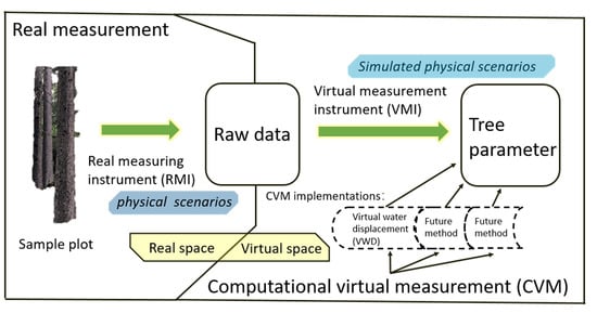
5.1. Computational Virtual Measurement

Human beings have been learning the law and experience from nature since ancient times and have known how to utilize physical rules to measure objects. The phenomenon of water displacement was discovered independently as Archimedes in Greek and in the story of Cao Chong weighing the elephant in China. Measuring methods connect certain features of the measuring target clearly with certain physical parameters. In a measuring method, no mathematical processes are employed to make predictions. Learning from the water displacement method in reality, we successfully developed the virtual water displacement method, which was aiming to directly measure the LiDAR point cloud for stem volume.

The key feature of VWD is to replace the mathematical processes on data with the simulating of physical principles on measuring instrument and measuring procedure. We further concluded this feature as a general and conceptional method, i.e., computational virtual measurement (CVM). The primary mechanism of CVM was described as follows:

To measure the data in a virtual space by simulating the physical mechanism of measuring instruments in reality.

CVM is a measuring method in a virtual space. No predictive mathematical processes are applied to the measuring target. Consequently, at the algorithmic level, no validation and calibration are required. The core process in a CVM method is simulating the physical mechanism of measuring instruments. Methods from a third-party physical simulation engine can be included to simplify the difficulty in method developing. CVM shifts and conceals the data processes in the physical simulation. For an end-user of CVM, they do not need to care about how to simulate the measuring instrument. The simulation process is a BlackBox for users, where the user can start the virtual measurement and wait for the measuring result.

5.2. Computer Performance and the VWD Feasibility in the Future

As shown in this study, compared to processing data directly, the simulating of measuring instruments was complicated. The quantity of points for a real tree may vary from 100,000 to 10,000,000, which far exceeds current computer performance, both in software and hardware. In a VWD process, both VWMs and tree points consume the resources of the rigid body. However, the quantity of the rigid body is limited by the physical engine, PhysX SDK 3.4. The maximum support of rigid bodies is 65,535 [52]. Compared to the regular quantity of points in a large tree point cloud. We did not have enough rigid bodies to replace the original points in a virtual space. Furthermore, compared to points in point clouds, VWMs consume much more rigid bodies in order to fill the vessel. Thus, the current physical engine cannot support a VWD process at a large tree level.

In addition to the limitation in software, physical simulation depends on computer hardware as well. It was useful to know how many rigid bodies could be supported by the desktop computer in this study. The quantity of VWMs had a negative relationship with the VWM diameter. For the consideration of computer performance, we intend to use fewer VWMs. However, the VWM diameter was proved to relate to the accuracy positively. Therefore, we had to perform VDM processes using small VWMs.

In order to find a favorable compromise with this contradiction, we used frames per second (FPS) as the criterion to evaluate the smallest VWMs we could use. We filled VWMs with different diameters. During those tests, if the FPS < 1 in the current VWD process, we stopped further tests to seek a potential smaller diameter of VWMs. For the vast vessel (no tree points), the smallest VWM diameter was 21.416 cm; for the vessel with tree points, the smallest VWM diameter was 29.136 cm. The graphics card we used was Nvidia GeForce GT 640 (2012), with a FP32 (float) performance of 693 GFLOPS. Comparing to this, the current high-end graphics card, NVIDIA GeForce RTX 2080Ti (2019), has a 13,450 GFLOPS in FP32 (float) and is ~19 times faster. The maximal VWMs that simultaneously existed in our VGE was 7227. We assumed that there is a simple linear relationship with FP32 and the number of rigid body support. Then, we could have ~130,000 (65,535) rigid bodies to be allocated if we used the NVIDIA GeForce RTX 2080Ti. Compared with the date of manufacture of those two graphics cards, which are 2012 and 2020. We could roughly foresee that the hardware would like to support VWMs and tree points at the quantity at 10,000,000 within the next ten years. Meanwhile, we are expecting the improvement of the PhysX SDK as well.

5.3. Scale Effect for VWMs

The scale effect is a phenomenon we discovered in the VWD processes when we tested the VWD measuring with regular shape objects. This phenomenon can help us to choose the optimal diameter of the VWM when the spatial scale of the measuring target is determined. The choice is simple. It is best to choose the smallest diameter VWM that the computer performance can support.

Figure 16a shows a VWD measurement using a small and a large VWM for the same measurement target. The ratio between the diameter of the external sphere of measurement target and the VWM diameter could be regarded as a quantitative indicator, if needed. Figure 16b shows one source of error caused by wrong ejections of VWM. The wrong ejection usually occurs at the top layers of the vessel. From a single VWM perspective, the VWM diameter has no influence on the likelihood of wrong ejections, if we count the quantity of VWM. Apparently, one wrong ejection of a small VWM has a less negative impact on the measuring process.

In addition to the phenomenon occurring at the top level, the motion of a single VWM in its adjacent area is also considered to be a factor affecting the measuring process. As shown in Figure 16c, each VWM has a randomly accessed region around its center, similar to the motion of real molecules. It is likely that there is a constant ratio between the volume (diameter) of the VWM and the size of this region. This is because all VWMs are driven by an identical physical scenario, regardless of the diameter. However, through virtual experiments, it was found that VWMs with smaller diameters had better performance than VWMs with larger diameters. The possible reason determined by us is shown in Figure 16d. In a space of the same size, the large VWM is affected by the forces from fewer (four) sources. Meanwhile, the small VWM is affected by the force from much more (twenty-four) sources. The more sources of force there are, the more likely it is that the direction and velocity of the combined force will converge to zero. Accordingly, as shown in Figure 16e, the small VWM may have a relatively much smaller randomly accessed region compared to the large VWM.

5.4. Objectivity, Current Limitations and Further Development

The VWD developed in this work served as a theoretical proof of the CVM. As a generic method, CVM was considered to have a high degree of objectivity. This objectivity was rooted in the design of the algorithm itself. The key to the high degree of objectivity was that CVM used simulated physical processes without predictive mathematical procedures. This workflow was also used by real measurement instruments. Accordingly, the justification of a CVM process was provided by repeated measurement instead of procedures including validation and calibration. Meanwhile, CVM brought us a side benefit, i.e., minimizing the demand of the skill of data processing. This character was expected to contribute to industrial utilization, e.g., the sample plot survey in NFI. Namely, VMI would be considered as the same kind of equipment as RMI.

By developing VWD, we found the implementation of CVM on desktop computers challenging due to limitations. It was possible to duplicate this work using supercomputers. However, it is envisioned that VWD (including other CVM implementations) will eventually be distributed with no special requirements or costs. A simple strategy is to keep waiting for the further development of computers and related hardware, e.g., lidar scanner. Meanwhile, it is worth to further develop the theory of CVM and to extend the deployment platform for CVM. For example, we could try to deploy VWD application on the embodied computer in lidar scanner and hope for a real-time VWD measurement in forests.

Another way is to employ conventional mathematical processing in CVM. As shown in the VWD, those processes were used to compensate the insufficient computer power. Although, this combination would reduce the objectivity of VWD (and CVM). However, we foresaw that the versatility (for trees) and convenience (for users) of VWD (and CVM) could be preserved. For example, the adjustment process in Equations (7) and (8) can be accomplished by the manufacturer of the VMI. Then, for the user, this VWD application would still working with a parameter free state. We recommend that manufacturers of RMI could be attentive to VMI also.

6. Conclusions

In this study, the initial assumption of a method that did not require human intervention or involvement had evolved into a generic approach, the CVM. Although, there were some limitations from the desktop computer hardware and software during the development of VWD, the feasibility of the overall mechanism of CVM was successfully proved. In addition to stem volume, VWD was capable to measure point clouds volume regardless of shapes. It inspired us to keep working toward the further development of CVM implementations. We believed that CVM was a method with a higher degree of objectivity on the algorithmic level. It avoided the mathematical interconversion from natural trees to model trees. We expect that CVM research and industrial implementation of CVM would thrive in the near future.

References

1. Purves, D.; Pacala, S. Predictive models of forest dynamics. Science 2008, 320, 1452–1453. [Google Scholar] [CrossRef] [PubMed]
2. Breidenbach, J.; Granhus, A.; Hylen, G.; Eriksen, R.; Astrup, R. A century of National Forest Inventory in Norway–informing past, present, and future decisions. For. Ecosyst. 2020, 7, 46. [Google Scholar] [CrossRef]
3. Hiley, W. The Forests of Suomi (Finland): Results of the General Survey of the Forests of the Country carried out during the Years 1921–1924. Emp. For. J. 1927, 6, 316–318. [Google Scholar]
4. Hackenberg, J.; Morhart, C.; Sheppard, J.; Spiecker, H.; Disney, M. Highly accurate tree models derived from terrestrial laser scan data: A method description. Forests 2014, 5, 1069–1105. [Google Scholar] [CrossRef] [Green Version]
5. Wang, C. Biomass allometric equations for 10 co-occurring tree species in Chinese temperate forests. For. Ecol. Manag. 2006, 222, 9–16. [Google Scholar] [CrossRef]
6. Fang, R.; Strimbu, B.M. Comparison of mature douglas-firs’ crown structures developed with two quantitative structural models using TLS point clouds for neighboring trees in a natural regime stand. Remote Sens. 2019, 11, 1661. [Google Scholar] [CrossRef] [Green Version]
7. Henry, M.; Bombelli, A.; Trotta, C.; Alessandrini, A.; Birigazzi, L.; Sola, G.; Vieilledent, G.; Santenoise, P.; Longuetaud, F.; Valentini, R. GlobAllomeTree: International platform for tree allometric equations to support volume, biomass and carbon assessment. iForest 2013, 6, 326–330. [Google Scholar] [CrossRef] [Green Version]
8. Zeng, W.; Tomppo, E.; Healey, S.P.; Gadow, K.V. The national forest inventory in China: History-results-international context. For. Ecosyst. 2015, 2, 23. [Google Scholar] [CrossRef] [Green Version]
9. Erez, T.; Tassa, Y.; Todorov, E. Simulation tools for model-based robotics: Comparison of bullet, havok, mujoco, ode and physx. In Proceedings of the 2015 IEEE International Conference on Robotics and Automation (ICRA), Seattle, WA, USA, 25–30 May 2015; pp. 4397–4404. [Google Scholar]
10. Hongpan, N.; Yong, G.; Zhongming, H. Application research of PhysX engine in virtual environment. In Proceedings of the 2010 International Conference on Audio, Language and Image Processing, Shanghai, China, 23–25 November 2010; pp. 587–591. [Google Scholar]
11. Saarinen, N.; Kankare, V.; Vastaranta, M.; Luoma, V.; Pyörälä, J.; Tanhuanpää, T.; Liang, X.; Kaartinen, H.; Kukko, A.; Jaakkola, A.; et al. Feasibility of Terrestrial laser scanning for collecting stem volume information from single trees. ISPRS J. Photogramm. Remote Sens. 2017, 123, 140–158. [Google Scholar] [CrossRef]
12. Liang, X.L.; Kankare, V.; Hyyppa, J.; Wang, Y.S.; Kukko, A.; Haggren, H.; Yu, X.W.; Kaartinen, H.; Jaakkola, A.; Guan, F.Y.; et al. Terrestrial laser scanning in forest inventories. ISPRS J. Photogramm. Remote Sens. 2016, 115, 63–77. [Google Scholar] [CrossRef]
13. Fan, G.; Nan, L.; Dong, Y.; Su, X.; Chen, F. AdQSM: A New Method for Estimating Above-Ground Biomass from TLS Point Clouds. Remote Sens. 2020, 12, 3089. [Google Scholar] [CrossRef]
14. Pueschel, P.; Newnham, G.; Rock, G.; Udelhoven, T.; Werner, W.; Hill, J. The influence of scan mode and circle fitting on tree stem detection, stem diameter and volume extraction from terrestrial laser scans. ISPRS J. Photogramm. Remote Sens. 2013, 77, 44–56. [Google Scholar] [CrossRef]
15. Jiang, A.; Liu, J.; Zhou, J.; Zhang, M. Skeleton extraction from point clouds of trees with complex branches via graph contraction. Vis. Comp. 2021, 37, 2235–2251. [Google Scholar] [CrossRef]
16. Lecigne, B.; Delagrange, S.; Taugourdeau, O. Annual Shoot Segmentation and Physiological Age Classification from TLS Data in Trees with Acrotonic Growth. Forests 2021, 12, 391. [Google Scholar] [CrossRef]
17. Xie, D.; Wang, X.; Qi, J.; Chen, Y.; Mu, X.; Zhang, W.; Yan, G. Reconstruction of single tree with leaves based on terrestrial lidar point cloud data. Remote Sens. 2018, 10, 686. [Google Scholar] [CrossRef] [Green Version]
18. Bournez, E.; Landes, T.; Saudreau, M.; Kastendeuch, P.; Najjar, G. From TLS point clouds to 3D models of trees: A comparison of existing algorithms for 3D tree reconstruction. In Proceedings of the 3D Virtual Reconstruction and Visualization of Complex Architectures, Nafplio, Greece, 1–3 March 2017; pp. 113–120. [Google Scholar]
19. Zianis, D.; Muukkonen, P.; Mäkipää, R.; Mencuccini, M. Biomass and Stem Volume Equations for Tree Species in Europe; Silva Fennica Monographs: Helsinki, Finland, 2005. [Google Scholar]
20. Bienert, A.; Hess, C.; Maas, H.; Von Oheimb, G. A voxel-based technique to estimate the volume of trees from terrestrial laser scanner data. Int. Arch. Photogramm. Remote Sens. Spat. Inf. Sci. 2014, 40, 101. [Google Scholar] [CrossRef] [Green Version]
21. Raumonen, P.; Kaasalainen, M.; Åkerblom, M.; Kaasalainen, S.; Kaartinen, H.; Vastaranta, M.; Holopainen, M.; Disney, M.; Lewis, P. Fast automatic precision tree models from terrestrial laser scanner data. Remote Sens. 2013, 5, 491–520. [Google Scholar] [CrossRef] [Green Version]
22. Calders, K.; Newnham, G.; Burt, A.; Murphy, S.; Raumonen, P.; Herold, M.; Culvenor, D.; Avitabile, V.; Disney, M.; Armston, J.; et al. Nondestructive estimates of above-ground biomass using terrestrial laser scanning. Methods Ecol. Evol. 2015, 6, 198–208. [Google Scholar] [CrossRef]
23. Delagrange, S.; Jauvin, C.; Rochon, P. PypeTree: A tool for reconstructing tree perennial tissues from point clouds. Sensors 2014, 14, 4271–4289. [Google Scholar] [CrossRef] [Green Version]
24. Du, S.; Lindenbergh, R.; Ledoux, H.; Stoter, J.; Nan, L. AdTree: Accurate, detailed, and automatic modelling of laser-scanned trees. Remote Sens. 2019, 11, 2074. [Google Scholar] [CrossRef] [Green Version]
25. Unity Technologies. Unity User Manual (2018.2). Available online: https://docs.unity3d.com/Manual/UnityManual.html (accessed on 23 November 2019).
26. Boeing, A.; Bräunl, T. Evaluation of real-time physics simulation systems. In Proceedings of the 5th International Conference on Computer Graphics and Interactive Techniques in Australia and Southeast Asia, Perth, Australia, 1–4 December 2007; pp. 281–288. [Google Scholar]
27. Zhang, C.; Chen, T. Efficient feature extraction for 2d/3d objects in mesh representation. In Proceedings of the IEEE 2001 International Conference on Image Processing (Cat. No. 01CH37205), Thessaloniki, Greece, 7–10 October 2001; pp. 935–938. [Google Scholar]
28. Åkerblom, M. Quantitative Tree Modeling from Laser Scanning Data. Master’s Thesis, Tampere University, Tampere, Finland, 2012. [Google Scholar]
29. Unity Technologies. Tree Editor. Available online: https://docs.unity3d.com/Manual/class-Tree.html (accessed on 23 November 2019).
30. Rusu, R.B.; Cousins, S. Point cloud library (PCL). In Proceedings of the 2011 IEEE International Conference on Robotics and Automation, Shanghai, China, 9–13 May 2011; pp. 1–4. [Google Scholar]
31. Schroeder, W.J.; Martin, K.M.; Lorensen, W.E. The design and implementation of an object-oriented toolkit for 3d graphics and visualization. In Proceedings of the Seventh Annual IEEE Visualization’96, San Francisco, CA, USA, 27 October–1 November 1996; pp. 93–100. [Google Scholar]
32. Hackenberg, J.; Spiecker, H.; Calders, K.; Disney, M.; Raumonen, P. Simpletree-an efficient open source tool to build tree models from tls clouds. Forests 2015, 6, 4245–4294. [Google Scholar] [CrossRef]
33. Batty, M. Virtual geography. Futures 1997, 29, 337–352. [Google Scholar] [CrossRef]
34. Lin, H.; Gong, J. Exploring virtual geographic environments. Geogr. Inf. Sci. 2001, 7, 1–7. [Google Scholar] [CrossRef]
35. Mekni, M. Automated Generation of Geometrically-Precise and Semantically-Informed Virtual Geographic Environments Populated with Spatially-Reasoning Agents; Universal-Publishers: Irvine, CA, USA, 2010. [Google Scholar]
36. Lin, H.; Chen, M.; Lu, G.; Zhu, Q.; Gong, J.; You, X.; Wen, Y.; Xu, B.; Hu, M. Virtual geographic environments (vges): A new generation of geographic analysis tool. Earth-Sci. Rev. 2013, 126, 74–84. [Google Scholar] [CrossRef] [Green Version]
37. Liang, J.; Gong, J.; Li, Y. Realistic rendering for physically based shallow water simulation in virtual geographic environments (vges). Ann. GIS 2015, 21, 301–312. [Google Scholar] [CrossRef]
38. Machado, S.d.A.; Nadolny, M. Comparação de métodos de cubagem de árvores e de diversos comprimentos de seção. In Anais do III Congresso Florestal e do Meio Ambiente do Paraná; Associaçáo Parananense de Engenheiros Florestais: Curitiba, Brazil, 1991; pp. 89–104. [Google Scholar]
39. Mestre, S.; Veye, F.; Perez-Martin, A.; Behar, T.; Triboulet, J.; Berron, N.; Demattei, C.; Quéré, I. Validation of lower limb segmental volumetry with hand-held, self-positioning three-dimensional laser scanner against water displacement. J. Vasc. Surg. Venous Lymphat. Disord. 2014, 2, 39–45. [Google Scholar] [CrossRef]
40. Damstra, R.J.; Glazenburg, E.J.; Hop, W.C.J. Validation of the inverse water volumetry method: A new gold standard for arm volume measurements. Breast Cancer Res. Treat. 2006, 99, 267. [Google Scholar] [CrossRef] [PubMed]
41. Maniatis, D.; Saint André, L.; Temmerman, M.; Malhi, Y.; Beeckman, H. The potential of using xylarium wood samples for wood density calculations: A comparison of approaches for volume measurement. iForest 2011, 4, 150. [Google Scholar] [CrossRef]
42. Unity Technologies. Scenes. Available online: https://docs.unity3d.com/Manual/CreatingScenes.html (accessed on 18 June 2018).
43. Hifi, M.; M’hallah, R. A literature review on circle and sphere packing problems: Models and methodologies. Adv. Oper. Res. 2009, 2009, 150624. [Google Scholar] [CrossRef]
44. Archer, T.; Whitechapel, A. Inside c#; Microsoft Press: Redmond, MA, USA, 2002; Volume 1. [Google Scholar]
45. Scherzer, D.; Bagar, F.; Mattausch, O. Volumetric real-time water and foam rendering. In GPU Pro 360 Guide to Rendering; AK Peters/CRC Press: Boca Raton, FL, USA, 2018; pp. 189–201. [Google Scholar]
46. Horvath, C.J. Empirical directional wave spectra for computer graphics. In Proceedings of the 2015 Symposium on Digital Production, Los Angeles, CA, USA, 8 August 2015; ACM: New York, NY, USA, 2015; pp. 29–39. [Google Scholar]
47. Bridson, R. Fluid Simulation for Computer Graphics; AK Peters/CRC Press: Boca Raton, FL, USA, 2015. [Google Scholar]
48. Dullweber, A.; Leimkuhler, B.; McLachlan, R. Symplectic splitting methods for rigid body molecular dynamics. J. Chem. Phys. 1997, 107, 5840–5851. [Google Scholar] [CrossRef] [Green Version]
49. Unity Technologies. Physics. Available online: https://docs.unity3d.com/Manual/PhysicsSection.html (accessed on 24 December 2018).
50. Nvidia Corporation. Rigid Body Dynamics. Available online: https://docs.nvidia.com/gameworks/content/gameworkslibrary/physx/guide/Manual/RigidBodyDynamics.html#applying-forces-and-torques (accessed on 24 December 2018).
51. Unity Technologies. Rigidbody. Available online: https://docs.unity3d.com/ScriptReference/Rigidbody.html (accessed on 24 December 2018).
52. Nvidia Corporation. Rigid Body Collision. Available online: https://docs.nvidia.com/gameworks/content/gameworkslibrary/physx/guide/Manual/RigidBodyCollision.html#broad-phase-algorithms (accessed on 25 December 2018).
53. Nvidia Corporation. Geometry Queries. Available online: https://docs.nvidia.com/gameworks/content/gameworkslibrary/physx/guide/Manual/GeometryQueries.html (accessed on 25 December 2018).
54. Unity Technologies. Mesh Collider. Available online: https://docs.unity3d.com/Manual/class-MeshCollider.html (accessed on 1 July 2021).
55. Huang, W.; Yu, L. Serial symmetrical relocation algorithm for the equal sphere packing problem. arXiv 2012, arXiv:1202.4149. [Google Scholar]
Figure 1. Regular shape objects and corresponding point clouds. (a) The cube model; (b) the sphere model; (c) the cylinder model; (d) the point cloud resampled the cube model; (e) the point cloud consisted of the original mesh vertices in the sphere model; (f) the point cloud resampled the cylinder model.
Remotesensing 13 04627 g001
Figure 2. 3D models and the corresponding point clouds of two types of artificial stems. (Left): the ”stem” model and its point cloud. (Right): the “stem with branches” model and its point cloud.
Remotesensing 13 04627 g002
Figure 3. Workflow for preparing artificial ground truths.
Remotesensing 13 04627 g003
Figure 4. The steps of the establishment of the virtual geographic environment (VGE) for virtual water displacement (VWD).
Remotesensing 13 04627 g004
Figure 5. The Key mechanism of VMI of VWD in this study, static and dynamic roles of virtual water molecules (VWMs): (a) a VWM acts as a placeholder that can occupy an exclusive space in the vessel; (b) the dynamic motion of the VWM. The VWMs are attracted by virtual gravity. At the same time, VWMs have physical interactions with each other.
Remotesensing 13 04627 g005
Figure 6. The demonstration of the similar response of VWMs for the solid tree model (left) and its corresponding point cloud (right).
Remotesensing 13 04627 g006
Figure 7. Theoretical (yellow) and full workflow for virtual water displacement (VWD) simulation.
Remotesensing 13 04627 g007
Figure 8. The spatial distribution of theoretical and actual filling of VWMs. The vessel is a cube with a side length of 400 cm; VWM diameter is 30.72 cm; (Left): the theoretical maximal filling (2916); (Right): the actual filling driven by PhysX (2431).
Remotesensing 13 04627 g008
Figure 9. The actual filling experiment of VWMs using different diameters from 21.416 to 43.245 cm in a vast vessel. (Left): The quantity difference between the theoretical and the actual with standard deviation; (Right): The relative difference between the theoretical and the actual with relative standard deviation.
Remotesensing 13 04627 g009
Figure 10. The mathematical relationship between the theoretical maximum and actual filling of VMWs. (Left): There is a simple linear relationship with the theoretical and the actual (r2 = 0.999); (Right): The theoretical and empirical k determined by Equations (5) and (6).
Remotesensing 13 04627 g010
Figure 11. A VWD process for a cube, side length is 100, VWM diameter is 29.136. (Left) Front perspective; (Right) bottom perspective.
Remotesensing 13 04627 g011
Figure 12. The filling using VWMs for cube (side length = 100 cm), cylinder (diameter = 100 cm, height = 200 cm), and sphere (diameter = 100 cm). (Left): The quantity difference between the actual maximal filling number and the filling number with standard deviation. (Right): The relative standard deviation for each filling was repeated five times.
Remotesensing 13 04627 g012
Figure 13. The VWD volume estimation for three regular shape objects with six different diameter VWMs. (Left): The quantitative difference between VWD volume and true volume. (Right): An additional coefficient using true volume dividing VWD volume.
Remotesensing 13 04627 g013
Figure 14. The VWD process for the artificial stem. (Left): The artificial point cloud in the standard cube vessel (side length = 400 cm) and VWMs (diameter = 29.136 cm); (Right): The artificial point cloud in a special cuboid (bottom length = 120 cm, bottom width = 60 cm, height = 300 cm) and VWMs (diameter = 10 cm).
Remotesensing 13 04627 g014
Figure 15. Scale effect of VWMs. (Left): VWMs (diameter = 29.136 cm) collide with the artificial point cloud (bottom view); (Right): VWMs (diameter = 10 cm) collide with the same point cloud (front view).
Remotesensing 13 04627 g015
Figure 16. Demonstration graph for scale effect and random movement of VWMs in micrographic scale. (a) VWD process on the same measuring target using small and large VWMs. (b) The wrong ejection occurred in the top (two) layers of the vessel. (c) Randomly accessed region around the center of VWM. (d) Source of forces that applied to the VWMs (in the center). (e) Adjusted randomly accessed region (the red circle) by the consideration of the source of forces.
Remotesensing 13 04627 g016