Article

Forest Structural Complexity Tool—An Open Source, Fully-Automated Tool for Measuring Forest Point Clouds

1
ARC Training Centre for Forest Value, University of Tasmania, Sandy Bay, TAS 7005, Australia
2
School of Information and Communication Technology, University of Tasmania, Sandy Bay, TAS 7005, Australia
3
Institute of Sustainable Industries and Livable Cities, Victoria University, Footscray, VIC 3011, Australia
4
Interpine Group Ltd., Rotorua 3010, New Zealand
5
PF Olsen (Australia) Pty Ltd., Ivanhoe, VIC 3079, Australia
*
Author to whom correspondence should be addressed.
Remote Sens. 2021, 13(22), 4677; https://doi.org/10.3390/rs13224677
Submission received: 5 October 2021 / Revised: 16 November 2021 / Accepted: 16 November 2021 / Published: 19 November 2021
(This article belongs to the Special Issue Advances in LiDAR Remote Sensing for Forestry and Ecology)

Abstract

:
Forest mensuration remains critical in managing our forests sustainably, however, capturing such measurements remains costly, time-consuming and provides minimal amounts of information such as diameter at breast height (DBH), location, and height. Plot scale remote sensing techniques show great promise in extracting detailed forest measurements rapidly and cheaply, however, they have been held back from large-scale implementation due to the complex and time-consuming workflows required to utilize them. This work is focused on describing and evaluating an approach to create a robust, sensor-agnostic and fully automated forest point cloud measurement tool called the Forest Structural Complexity Tool (FSCT). The performance of FSCT is evaluated using 49 forest plots of terrestrial laser scanned (TLS) point clouds and 7022 destructively sampled manual diameter measurements of the stems. FSCT was able to match 5141 of the reference diameter measurements fully automatically with mean, median and root mean squared errors (RMSE) of 0.032 m, 0.02 m, and 0.103 m respectively. A video demonstration is also provided to qualitatively demonstrate the diversity of point cloud datasets that the tool is capable of measuring. FSCT is provided as open source, with the goal of enabling plot scale remote sensing techniques to replace most structural forest mensuration in research and industry. Future work on this project will seek to make incremental improvements to this methodology to further improve the reliability and accuracy of this tool in most high-resolution forest point clouds.

Graphical Abstract

1. Introduction

Remote sensing technologies are revolutionizing the way forests are measured in many ways; however, at plot scales, manual forest mensuration with simple tools remains commonplace in industry and research. While the high initial cost of remote sensing tools such as light detection and ranging (LiDAR) likely slows their uptake, the capture of high-resolution point clouds is becoming increasingly efficient and scalable, while equipment costs are declining. Mobile laser scanning (MLS) [1,2,3,4], terrestrial [5,6,7,8] and aerial [9,10] close-range photogrammetry (TP and AP) and terrestrial laser scanning (TLS) [11,12,13,14,15,16,17,18,19,20,21,22,23] are capable of generating high accuracy and high-resolution point clouds of forests considerably faster than a human could measure them manually. While forest point clouds can be captured relatively quickly, they are simply an array of points in 3D space; thus, they can be of limited use without further processing. To make such point clouds more broadly useful, a means of rapidly, efficiently, and ideally, automatically extracting meaningful information from them is required. Many fields could benefit from improved forest measurement capabilities, including forestry, conservation [24], restoration, habitat management [25,26], climate change and carbon stock monitoring [27,28,29], bushfire management and monitoring [30] and more [31]. Planet-scale remote sensing technologies have shown a lot of promise for mapping our forests at relatively low-resolutions [29,32,33]; however, high-quality field references remain necessary to ensure the validity of these large-scale models, both during development and over time, as our climate and environmental conditions change. High-resolution point clouds hold the potential to be used as high-quality inputs to these models and can be considerably more efficient to capture than conventional field reference information, while simultaneously capturing far greater detail than simple measurements could capture. While there are many potential uses for these high-resolution point clouds, reliable and fully automated measurements from such point clouds are required to make widespread adoption both feasible and practical.
While numerous approaches and tools for extracting information from high-resolution forest point clouds have been described in the past [15,17,34,35,36,37,38,39,40,41,42,43,44,45,46,47,48,49,50,51,52,53,54,55,56], uptake is still relatively limited in the forestry industry and in applied forest research. This limited and lagging uptake suggests that there are still important practical challenges to overcome in replacing diameter tapes and calipers with more advanced tools such as LiDAR and photogrammetry. With many of the existing point cloud tools and approaches, it is common to require complicated and/or time-consuming workflows, manual tuning of parameters, combinations of multiple methods (requiring software development skills), or re-implementation of methods from papers. Further, highly-complex forest structures, commonly present in native Australian forests, present considerable challenges to such tools. For these reasons, our goal was to develop an easy-to-use, open-source tool to turn diverse and complex, high-resolution forest point clouds into a set of simple outputs fully automatically and without manual tuning of parameters. In this paper, we present the first version of our Python package called the Forest Structural Complexity Tool (FSCT). This tool may be gradually improved upon and updated over time, with the goal of making a highly-robust tool, which can fully automatically extract directly useful information from point clouds captured using TLS, MLS, very-high-resolution aerial laser scanning (ALS) and high-resolution photogrammetry, even in highly complex forests. This paper does not seek to evaluate the performance of FSCT relative to other existing tools; instead, FSCT is evaluated against a large-scale set of manually collected reference measurements. While a comparison against other point cloud tools would be interesting, FSCT was created out of a need for fully automated and reliable plot measurements from complex and diverse forest point clouds, which was not satisfied by our searches of the relevant literature, nor by our testing of existing software.
Our approach involves initially using a deep learning technique based upon Pointnet++ [57] to semantically segment forest point clouds into four categories: terrain, vegetation, coarse woody debris (CWD) and stems. This deep learning approach was trained with the goal of working on structurally diverse point clouds captured using most high-resolution point cloud generation techniques. This approach was described and evaluated in our previous paper [58], and forms the starting point from which this paper continues. This paper describes how we exploit the segmented point cloud to extract highly detailed measurements from forest point clouds, both robustly and completely automatically on point clouds from multiple sensor types. We believe that this tool makes it practical for manual forest mensuration of structural features to be replaced with plot scale remote sensing techniques, due to its ability to function in high levels of structural complexity, where prior existing tools were less effective or required considerable amounts of parameter tuning and/or manual corrections to be effective.
One of the major differences of our approach to others in the literature is that we obtain measurements before sorting points into individual trees, rather than identifying individual trees and then measuring them. This approach allows the tool to exploit the orientation information of the branches/stem segments to segment them into individual trees, even in the presence of considerable occlusions in the data. By exploiting the semantically segmented point clouds, the vegetation, terrain and CWD classes are simply ignored when taking initial measurements of the trees, allowing considerable robustness to high levels of structural complexity. The details of this approach are discussed in the following section.

2. Materials and Methods

This methodology is broken up into seven sections. First, we present a condensed explanation of the workings of FSCT. This explanation does not cover every detail of the implementation; however, it is intended to provide an overview of the important concepts and approaches used. If further information is required, the code and relevant documentation are made openly available on GitHub here: https://github.com/SKrisanski/FSCT (Date Accessed: 19 November 2021). The second and third sections describe the collection and scope of the destructively sampled reference datasets and the TLS point clouds, respectively. The fourth and fifth sections describe the automated measurement validation process and a qualitative video demonstration of the tool on additional datasets. The sixth section describes the computational resources used. Lastly, the additional outputs of FSCT beyond stem measurements are described.

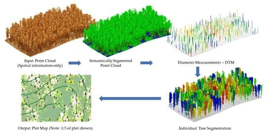
2.1. Forest Structural Complexity Tool Overview

This work builds upon our previous paper [58], relying upon the semantically segmented point clouds as a starting point for our other algorithms. Figure 1 shows a schematic diagram of how FSCT is designed, and how it is connected to our previous semantic segmentation paper. This approach to forest measurement was developed with the goal of being fully automated, and robust to structurally complex and diverse forest point clouds captured using most types of high-resolution remote sensing techniques. Suitable point clouds can be from MLS, TLS, both aerial and terrestrial close-range photogrammetry (AP/TP), and even high-resolution ALS.
In the context of this paper, “high-resolution” is used to refer to a point cloud with sufficient accuracy, precision, completeness of coverage, and point density with which one could reasonably expect to measure the diameter of a stem. Based on informal testing of this tool on a variety of datasets, high-resolution ALS data is on the borderline of functionality, so only the highest resolution ALS datasets are suitable for the tool in this version. Figure 2 provides an indication of the minimum point density that the point clouds must be for FSCT to function as intended.
As point density reduces below what is shown in Figure 2, the stems will be incorrectly segmented as part of the vegetation class. As FSCT is reliant upon the semantic segmentation step, FSCT cannot detect a stem unless the segmentation process accurately labels it as a stem.

2.1.1. Point Cloud Semantic Segmentation

The first major step of the tool is to perform semantic segmentation of the point cloud using the method described in our previous paper [58]. This uses a point cloud deep learning technique based on the Pointnet++ [57] architecture to segment the point clouds into four categories: terrain, vegetation, CWD and stems. Please see the previous paper for details, or the code for the implementation.

2.1.2. Digital Terrain Model

The second step is to use the terrain points extracted by the segmentation model as input to create a digital terrain model (DTM). The DTM method described in our previous work [58] was modified to reduce RAM consumption and to improve reliability/robustness on steep terrain. Our new DTM algorithm prioritises the use of the terrain segmented points, but if insufficient terrain points are present in an area, it will use the vegetation, stem and CWD points instead. While the altered DTM implementation is not the focus of this paper, it is available in the provided code.

2.1.3. Point Cloud Cleaning after Segmentation

The height of all points relative to the DTM are computed, allowing us to relabel any stem, CWD and vegetation points which are below the DTM height + 0.1 m as terrain points. Any CWD points above 10 m over the DTM are also removed, as, by definition, the CWD class is on the ground; therefore, any CWD points above 10 m would be incorrectly labeled in almost all circumstances. Any terrain points greater than 0.1 m above or below the DTM are also considered erroneous and are removed.

2.1.4. Stem Point Cloud Skeletonization

Before the method is described, we will define our coordinate system with the positive Z-axis pointing in the upwards direction. The orientation of the X and Y axes do not matter in this method, other than being within the plane of the horizon. The first step of the skeletonization process is to slice the stem point cloud into parallel slices in the XY plane. The point cloud slices are then clustered using the hierarchical density based spatial clustering for applications with noise (HDBSCAN) [59] algorithm to get clusters of stems/branches in each slice. For each cluster, the median position in the slice is calculated. These median points become the skeleton shown in the right of Figure 3. For each median point that makes up the skeleton, the corresponding cluster of stem points in the slice is set aside for the next step. This is visualised in Figure 3.

2.1.5. Skeleton Clustering into Branch/Stem Segments

These skeletons are then clustered using the density based spatial clustering for applications with noise (DBSCAN) algorithm [60,61], with an epsilon of 1.5× the slice increment, which has the effect of separating most of the individual stem/branch segments into separate clusters. This value of epsilon was chosen through experimentation. If the epsilon is too large, the branch segments would not be separate clusters, and if it is too small, clusters would be too small for the cylinder fitting step. Points considered outliers by the clustering algorithm are then sorted to the nearest group, provided they are within a radius of 3× the slice-increment value of any point in the nearest group. The clusters of stem points, which were set aside in the previous step, are now used to convert the skeleton clusters into clusters of stem segments as visualised in Figure 4.

2.1.6. Cylinder Fitting

The skeleton clusters and corresponding stem segment clusters are passed to the cylinder fitting function. Singular value decomposition (SVD) is used on each skeleton cluster to obtain a vector representing the major axis of the stem/branch segment. Starting from the lowest skeleton point, the five nearest neighbors are found. These points define the locations of two planes perpendicular to the major axis. The stem/branch segment is sliced between these two planes to get ideally circular slices of points from the stem/branch. These sets of points are rotated using Rodrigues rotation from the major axis to the Z-axis (up). Two-dimensional random sample consensus (RANSAC) [62] circle fitting is applied to these sets of points in the X and Y axes to extract the circle centre, radius, and the Circumferential Completeness Index (CCI) defined in [9]. A cylinder is only kept if the CCI is greater than 0.3 in order to reject a large number of poorly fitted cylinders. These processes are most easily understood visually in Figure 5.
Once the first set of neighboring points has been processed, the lowest point in the skeleton is removed, and the process is repeated until there are less than five skeleton points remaining (i.e., all skeleton points have been used). The result is a number of unsorted cylinders defined by the fitted circles and the major axis of each skeleton segment. These cylinders must be now sorted into individual trees.

2.1.7. Sorting Cylinder Measurements into Individual Trees

The sorting process consists of two main stages. The first stage assigns tree identification (Tree_ID) numbers to the individual measurements. This step is described in Algorithm 1 and visualised in Figure 6.
Algorithm 1. Cylinder Sorting Algorithm Part 1.
  •  Start with an array of cylinders represented by a point with X, Y, Z coordinates, a major axis vector (Vx, Vy, Vz), radius, CCI, cluster number, and Tree_ID (currently set to 0). We will call this array “unsorted_points”.
For clarity, we will label a variable “TREE_ID” as uppercase and the tree_id belonging to a cylinder point as “assigned_tree_id”.
2.
 Create another array called “sorted_points”.
Loop until unsorted_points is empty.
  •  Find the lowest point in unsorted_points. We will call this the “current_point”.
  •  If current_point’s assigned_tree_id equals 0:
    4.1.
     Set current_point’s assigned_tree_id to the value of TREE_ID.
    4.2.
     Increment the variable TREE_ID by 1.3.
    4.3.
     Move current_point from unsorted_points to sorted_points.
  •  Find all points in unsorted_points within search radius of current_point. For all of these points:
    5.1.
     Find the angle between the major axis vectors of point 1 and point 2.
    5.2.
     If angle is within angle_tolerance: continue.
    5.3.
     Find the angle between the translation vector from point 1 to point 2 and the major axis vector of point 1. If this angle is within the valid search angle range: assign the assigned_tree_id of point 1 to the assigned_tree_id of point 2.
This initial sorting process results in the measurements being grouped at the individual tree level; however, there are typically some groups which need re-sorting. The second part of the measurement sorting process is focused on handling the small clusters of measurements which were incorrectly identified as individual trees. This step runs through all of the clusters that potentially could be individual trees after sorting into groups in the previous step. These clusters will either be left as a tree or meet the requirements to be assigned to an existing tree or will be removed. The process is described in Algorithm 2 and visualised in Figure 7.
Algorithm 2. Cylinder Sorting Algorithm Part 2
  •  Start with array of sorted cylinder points (output from Algorithm 1).
  •  For each tree cluster identified in the previous sorting step:
    2.1.
     Search for cylinder points within a search radius of the lowest point of the current tree cluster.
    2.2.
     Find cylinder points within a specified “search_angle” of the major axis of the lowest point.
    2.3.
     If other tree points are found, the current tree_id is assigned the same tree_id value as the lower tree cluster.
    2.4.
     If no other tree points are found, the same process above is applied from the highest point of the current tree cluster.
    2.5.
     If still no other tree points are found, AND the lowest point of the current cluster is below 5 m above the ground, the current tree is kept. If the lowest point is not below 5 m above ground, it is deleted.

2.1.8. Cylinder Measurement Interpolation

Please note: the following steps are operating on individual trees rather than all trees at once. At this stage of the processing, the cylinder measurements are sorted into individual tree clusters, however, there will be gaps in the cylinder measurements/points as seen in Figure 7. It is necessary to interpolate between these gaps in cylinder points to represent the tree metrics more accurately. For the sake of brevity, a summary of the concept is described here instead of the exact implementation. When interpolating across these gaps, it is common for a small branch to be interpolated to a larger stem. If a linear interpolation was used for the radius value, a small branch would appear as a steeply angled cone when interpolating to a larger stem, which is unlikely to be realistic. For this reason, the smallest radius of the two cylinders is used to interpolate between measurements rather than a linear interpolation from one radius to the other. The X, Y and Z coordinates are linearly interpolated, and the major axis vector is set as the norm of the displacement vector from one cylinder point to the other (i.e., in the direction of a straight line connecting both cylinder endpoints).
As occlusions are common in forest point clouds, the lowest portion of a tree may be missing from the point cloud. To address this, and to enable a DBH estimate for all detected trees, FSCT uses the lowest diameter measurement of a detected tree, and vertically projects this diameter down to the DTM. It is generally a safe assumption that a tree will be connected to the ground, however, it is possible for a large hanging branch to be incorrectly treated as a standalone tree from this behaviour. It is important to note that we chose not to extrapolate the stem diameters to estimate DBH, as such extrapolations can be severely influenced by a bulge in a tree or a minor measurement error, leading to either a wide based frustum or tapering to an unrealistically narrow or even negative diameter base in some cases, which is a nonsensical result. The X, Y coordinates were also not extrapolated, as it is a reasonably safe assumption for most trees that the base is approximately straight down. Further, extrapolating from a small error in position/angle can also lead to a larger error than just going straight down. Extrapolations for both the diameter and position were tried during development, but the simplest solution of using the lowest diameter and going straight down was found to have far more predictable and reasonable behaviour. The exact implementation is available in the code if further information is required.

2.1.9. Cylinder Measurement Smoothing and Cleaning

The cleaning process removes overlapping measurements and applies smoothing to the cylinder measurements. This cleaning and volume extraction process operates on sets of cylinders belonging to individual trees. The first step is radius smoothing; thus, for each cylinder, its radius is changed to the median radius of the 10 nearest neighbour cylinders. Next, the cleaning process starts with the lowest cylinder of a tree and finds all neighbouring measurements within a specified radius, referred to as “cleaned_measurement_radius” in the code. Of those neighbours, the median radius, major axis vector, and positions of the measurements within the top 50% of CCI values (of the neighbouring measurements) are assigned to a single point, while the rest of the neighbours are deleted. This process is repeated until only the averaged points remain, effectively smoothing and cleaning the measurement outputs.

2.1.10. Stem Volume Extraction

The volume extraction step is built into the smoothing/cleaning step described in Section 2.1.9. and so also operates on sets of cylinders belonging to a single tree. This process occurs after the cleaning and smoothing step. Starting from the lowest cylinder point, the nearest neighbour cylinder point is identified. Using the distance between the cylinder centres and the two radii belonging to the two points, the frustum volume is calculated. The lowest point is removed, and the process repeats until all cylinder points have been used. The frustum volumes are summed up, and the result is an estimate of the total stem/branch volume of that tree.

2.1.11. Individual Tree Segmentation of Vegetation and Stem points

The vegetation sorting process either assigns the vegetation points (labelled in the semantic segmentation step) to understory vegetation, individual trees or, in the event that points do not meet the criteria for assignment, deletes them. The first step is to separate the understory vegetation from the canopy, so all vegetation points below a user configurable height (we used 3 m) above the DTM are set aside as understory points. The tree ID of the nearest cylinder measurement (2D distance in X, Y axes) within a user configurable range (we use 1 m) is assigned to each of the vegetation points. Any vegetation points which were not assigned to a tree are deleted. An example of the results of the vegetation point sorting output is shown in Figure 8.
The optional stem point sorting process is similar to the vegetation sorting process; however, it differs in that it finds the nearest cylinder measurement in a 3D distance rather than the 2D distance used for vegetation. Like the vegetation sorting process, a user-configurable parameter controls the maximum distance to search (we used 1 m in this study, though this occurs after the measurement process and is not critical for standard use cases). The stem sorting process is an additional output that is not used in this paper; however, this addition means that complete, individually segmented trees are readily available should future research using FSCT require them.
Both of these sorting approaches are rather simplistic in their current form, so usage of the individually segmented trees for training datasets will likely require some manual corrections to be made. These simplistic individual tree segmentation approaches were designed to work acceptably well on most high-resolution forest point clouds; however, this comes with the trade-off that these simple assumptions do not always hold true. For example, by assigning vegetation points to the nearest stem in 2D, the tool is able to extract tree heights from photogrammetry point clouds with occlusions and significant gaps between the lower stems and the canopy. However, this comes at the price of overestimating the height of small trees under closed canopies, by incorrectly assigning the canopy directly above these small trees to them. As this tool is intended to work with highly variable and imperfect datasets, an approach which works optimally in all situations is difficult to achieve; thus, until superior generalizing approaches are developed (likely deep learning based) or reliably complete point clouds without occlusions are consistently and easily attainable, these compromises are required.
Figure 8. Initially, any vegetation points less than 3 m above the DTM are classified as understory (black points). The remaining vegetation points are assigned to be the same tree as the nearest cylinder measurement in X and Y coordinates, provided that they are within a horizontal radius of 1 m (this can be adjusted). If there are no cylinders within a 1 m radius, the points are deleted. The trees shown above are coloured by their assigned Tree ID. Please note that adjacent trees may appear to be labelled as the same colour (due to random colour assignment), however, they were all successfully separated as different trees in this example.
Remotesensing 13 04677 g008

2.1.12. Automated Height Measurement Extraction

To extract the tree heights, the points representing cylinder measurements and the assigned vegetation points are combined at the individual tree level. The highest of these points is taken as the height measurement.

2.1.13. Automated Diameter at Breast Height (DBH) Measurement Extraction

The DBH (nominally 1.3 m above the ground) used in the analysis of this tool, is calculated by taking the mean diameter and X, Y position of all cylinder measurements (including projected measurements) between 1.0 m and 1.6 m above the DTM on a per tree basis. This means that even if the lower section of the tree is missing, FSCT will use higher up cylinder measurements, which have been projected to the ground, as the DBH measurement. Please see Section 2.1.8 for greater details of this projection step.

2.2. Reference Data Collection—Destructively Sampled Manual Field Measurements

A total of 49 Eucalyptus globulus plantation plots, 27 in Western Australia and 22 in the Green Triangle region, were measured by PF Olsen (Aus) Pty. Ltd. to collect data for the development of taper and growth models. Figure 9 shows the location of the sites in Australia.
The 49 plots were associated with and located adjacent to permanent sample plots and represent plantations established between 2000 and 2017. Each plot was circular and of a 0.04 ha area. All trees within the plot were measured for DBH using diameter tape over bark and height using a Haglöf Vertex hypsometer. From each plot, 12 trees representing the plot diameter range were selected at random for destructive sampling and were measured for diameters at a series of heights: 0.1, 0.3, 0.8, 1.3, 2.0, and then at 1.5 m increments from 2 m up using diameter tape over bark. This resulted in a dataset of 7022 diameter measurements collected from 588 trees. The locations of these trees were established using bearings and distances from a fixed plot centre marker. In some cases, an expert geographical information system (GIS) operator made manual adjustments to these tree locations in conjunction with the TLS point clouds of the plots, which were also referenced to the fixed plot centre marker. Summary information of the plots is available in Table 1 and Table 2 for the Western Australia and Green Triangle sites, respectively.

2.3. Data Collection—Terrestrial Laser Scanning of Plots

The point clouds of the plots were collected using multi-scan TLS with 5 to 8 scanning positions per plot. The number of scans varied depending on the conditions of each site and were decided at the discretion of the operator. The Green Triangle (GT) plots were scanned by Gertzel Pty Ltd. (Dingley Village, Victoria 3172, Australia) using a Riegl VZ 400i LiDAR (RIEGL Laser Measurement Systems GmbH, Austria), and the Western Australia (WA) sites were scanned by BCE Surveying Pty Ltd. (Bunbury, Western Australia 6230, Australia) using a Riegl VZ 1000 LiDAR. The point clouds were provided in *.LAS format using the Geocentric Datum of Australia (GDA) 1994 coordinate system with the GT dataset in the Map Grid of Australia (MGA) zone 54 and the WA dataset in MGA zone 50.

2.4. Validation Process—Comparing Manual and Automated Point Cloud Measurements

2.4.1. Tree Matching

For each manually measured reference tree, all automatically measured trees’ base coordinates within a 3 m radius are found. From these, the tree with the smallest difference in DBH is chosen and removed from the pool of available trees. This prevents the double counting of trees and is effectively the same method as used in [18]. This process is repeated until all trees are sorted. If no unique tree is present within 3 m of a reference tree, it is considered missing. Only the measurements of successfully matched trees could be meaningfully compared.

2.4.2. Taper Measurement Matching

The destructively sampled measurements of diameter were collected on the largest diameter of the tree at each measurement height. This results in a single taper profile for each individual tree and does not account for forked trees or branches. As this is a simplification of reality, it is necessary to extract similar simplified measurements from the FSCT output for each tree. Therefore, for comparison against the reference, the largest cylinder within ±0.2 m of each respective measurement height (relative to the DTM) for each given tree was used. For example: for a measurement height of 2.0 m, the largest cylinder in the tree between 1.8 m and 2.2 m above the DTM would be used in the comparison.

2.4.3. Reference Volume

The reference volumes were calculated from the reference taper measurements by summing the frustum volume between each measurement. This is a single stem model; thus, it would typically underestimate the true volume of a stem, due to not accounting for branching or forking.

2.4.4. Plot Density

The reference plot density was calculated by dividing the number of trees by the area (0.04 ha) of each plot. FSCT calculates this in the same way; however, it relies upon the detected trees and a specified plot radius. If no plot radius is specified, FSCT will use the area of a 2D (X, Y) convex hull of the DTM, as the DTM is cropped to the point cloud shape.

2.5. Qualitative Demonstration of FSCT on 5 Sensor/Structure Diverse Point Clouds

The validation data used in this study was only of a single, mostly even aged species (eucalyptus globulus). Collection of additional reference datasets was beyond the scope of this paper, so in order to demonstrate both the efficacy and the limitations of FSCT on point clouds of greatly varying structure and sensing techniques, five additional diverse point clouds were processed using FSCT. These point clouds are shown in an accompanying video. The five-point clouds are of the following sensor techniques and species combinations: fused above (nadir) and below canopy (close range) UAS photogrammetry (eucalyptus marginata), backpack-mounted MLS (pinus radiata), ALS (pinus radiata), above canopy (nadir only) UAS photogrammetry (eucalyptus amygdalina), and TLS (araucaria cunninghamii). Qualitative descriptions of notable moments in the video are provided.

2.6. Computer Hardware Used for Run times

All development, testing and evaluation of FSCT was performed on a desktop computer with an Intel i9-10900K central processing unit (CPU), 128 GB of DDR4 random access memory (RAM), and an Nvidia Titan RTX graphics processing unit (GPU). While the computer used to process this data is relatively high end, most recent gaming computers with an Nvidia GPU will be able to use FSCT, provided the plot size is small enough to meet the RAM requirements. This tool is computationally expensive to run; however, because it is fully automated, it allows a user to simply select a batch of “.las” format point clouds, or a directory containing the point clouds, and let the computer work through them without intervention. Processing the 49-point cloud datasets used in this study took approximately 3 days on the above-mentioned computer, using 18 of the 20 cores to keep the machine responsive for other work.
2.7 Additional Measures Provided by FSCT
While the main focus of this paper is to describe and evaluate the tree measurement processes, FSCT provides additional outputs which may be useful, but are not yet validated against field data. All segmented points are extracted as separate point clouds for ease of inspecting segmentation performance, and ease of creating additional training data to refine future semantic segmentation models. A plot map showing the stem locations, CWD points, understory vegetation, and contour map of the local terrain is generated as shown in Figure 10. The following additional metrics are also calculated by FSCT: canopy gap fraction, understory vegetation fraction, coarse woody debris coverage fraction, average gradient of plot, summary statistics of the measured trees, number of points of each segmentation class and run times of each section of FSCT.

3. Results

3.1. Diameter at Breast Height (DBH)

A comparison of the manual reference DBH against the automatically extracted measurements is visualised in Figure 11. Mean, median and RMS DBH errors were −0.007 m, 0.008 m and 0.072 m respectively. Of the 588 reference trees, 535 or 90.98% were successfully detected by FSCT. The mean and median errors are within the expected error of the reference diameter measurements, suggesting minimal bias.

3.2. Tree Height

The mean, median and RMS tree height errors were −0.139 m, −0.327 m and 3.524 m respectively as shown in Figure 12. FSCT appears to slightly underestimate height relative to the reference measurements, with a bias of −0.139 m; however, it is common for TLS to not fully capture the top of trees [64,65], and this is also within the expected error of hypsometer-based height measurements [66].

3.3. All Stem Diameter Measurements

Out of a total of 7022 reference diameter measurements, 5141 were matched to automatically measured TLS point cloud-based measurements. The mean, median and root-mean-squared (RMS/RMSE) diameter errors were +0.032 m, +0.02 m, and 0.103 m, respectively. This is visualised in Figure 13.

3.4. Tree and Measurement Detection Completeness

The measurement completeness (the fractions of measurements detected out of the total number of reference measurements) are shown in Figure 14. On the left, the completeness for reference tree detection is shown, and on the right, the completeness of all diameter measurements is shown. The tree detection completeness for 32 plots was between 0.95 and 1.0, with one plot (Plot 38) failing to detect any trees. Out of 49 plots, 30 had all trees detected. The mean and median completeness values for tree detection were 0.91 and 1.
The measurement detection completeness was expected to be less than the tree detection completeness, as a tree detection requires only a few measurements (below 10 m above the DTM) to be successful, while matched diameter measurements require successful measurement at a specific measurement height on a specific tree. No plots matched every single reference measurement; however, 32 plots had greater than 70% of reference measurements successfully matched. The mean and median completeness values for individual taper measurement detection were 0.71 and 0.76. Please see Table A1 and Table A2 in the Appendix A if additional details are desired.
Figure 14. Left shows the distribution of completeness for the plots (from a total of 49 plots). The histogram bins show how many plots had a given fraction of reference trees successfully detected by FSCT (i.e., 32 plots had a tree detection completeness between 0.95 and 1.0). Right shows the distribution of completeness for all reference diameter measurements successfully detected/matched with FSCT outputs.
Remotesensing 13 04677 g014

3.5. Stem Volume

The mean, median and RMS errors of stem volume relative to reference were −0.678, −0.467 and 1.669 m3. Given the simplistic, single stem approximation used to calculate the reference volume, the wide spread of the results is expected, however, these results provide a sanity check that the volume estimates appear reasonable. FSCT appears to underestimate volume with a bias of −0.678 m3 as seen in Figure 15.

3.6. Stem Density Estimates

FSCT was able to predict the plot density with a mean, median and RMS errors of −13, 67 and 256 stems per hectare. Some of the younger plots performed poorly due to failing to accurately segment and thus detect the stems. This number is also expected to have a reasonably large error relative to reference, as in the case of a 0.04 hectare plot: detecting 32 trees would give a result of 800 stems/ha, a single tree difference (31 or 33) in such a plot would mean ±25 stems/ha. This is shown in Figure 16. Small errors in stem counts are magnified on small plot scales. Larger scale plots would enable a more accurate assessment of stem density.

3.7. Run Times

FSCT is a computationally expensive program to run; thus run times of the reference plots on the hardware described in Section 2.6 are provided below in Figure 17. The largest contributor to run time is the measurement process, with measurement run times ranging from 0 min (plot 38 where no stems were correctly segmented), up to 60 min. The measurement run time depends on the number of stem-labelled points more than the total number of points in a point cloud, as a point cloud can have a lot of vegetation points and few stem points (taking a short time to measure), or have few vegetation points and a lot of stem points (taking a long time to measure). The pre-processing, semantic segmentation, and post-processing steps were dependent on the total number of points in the point cloud.

3.8. Video Demonstration of FSCT on Other Point Cloud Datasets

In addition to a quantitative evaluation of the performance of FSCT, a video is provided to qualitatively demonstrate the efficacy and limitations of FSCT on a broader range of point cloud datasets from a variety of high-resolution mapping tools and techniques. The tool is demonstrated on 5 datasets including combined above and below canopy UAS photogrammetry in dense and complex native Australian forest, MLS using a Hovermap sensor, ALS from a Riegl VUX-1LR LiDAR on a pinus radiata plantation, above canopy UAS photogrammetry in an open Australia native forest, and TLS of araucaria cunninghamii. The video is provided here: https://youtu.be/SIpl5HVqWcA (Date Accessed: 19 November 2021) and Figure 18 visualises the diversity of the datasets in the video. Qualitative notes with timestamps are provided in Appendix B.

4. Discussion

In the DBH comparison, there was a sub-centimeter bias in the FSCT-based measurements. Loose and hanging bark was common in this dataset and this was typically classified as part of the stem by the segmentation model, as can be seen in Figure 3. This hanging bark interferes with the diameter measurements in some situations, contributing to diameter measurement errors. In some cases, occlusions of the lower stem were present such that DBH could not be directly measured, so the automated DBH was based upon diameter measurements further up the stem, also contributing to DBH and other diameter measurement errors. Measurements from higher up the stems were more frequently incorrect or missing. This would be explained by a combination of factors such as canopy movement during capture in the event of a light breeze, denser vegetation being present (the canopy), smaller stem sections and branches, the effect of occlusions reducing point density and completeness towards the upper canopy, and beam divergence effects becoming more significant. All of these factors result in more difficult measurement conditions for any algorithm or set of algorithms to contend with, so at least some performance degradation further up the stems is to be expected.
The height measurements were consistent across the range of tree heights surveyed, pendixwith a tendency to slightly underestimate the tree heights relative to the reference. In terms of the accuracy of the reference tree heights, [66] studied the accuracy of the Vertex III hypsometer, finding it to be on the order of 0.2 to 0.3 m; thus, some height error could be explained as error in the reference information capture. FSCT’s height accuracy was within this error estimate, with a small underestimation bias relative to the reference. Other studies of measuring tree height with TLS [64,65] have found that TLS may not always capture the highest point of the canopy due to occlusions (from ground-based capture), which may also play a small role in the height underestimation.
As a result of designing the tool for generalisability on diverse forest point clouds, a notable trade off was made with the vegetation assignment process. Vegetation points are assigned to the nearest cylinder measurement point in 2D (X, Y), and as these are used in the height measurement process, the result is that small trees under a closed canopy will be assigned vegetation points from the closed canopy directly above them. Other, more complex approaches were attempted during development, but this simple approach was the only one which was able to provide reasonable and predictable height measurements under most circumstances when there are significant gaps/occlusions between the lower sections of the stem and their canopies. Such occlusions and gaps are particularly common in UAS photogrammetry datasets as seen in the qualitative video demonstration.
The automated measurement matching process, which matches reference trees to the automatically detected trees, is likely to result in some tree-mismatches; however, manually matching 588 individual trees was not considered to be necessary for the scope of this project. This will be a source of error in both the diameter and height measurements. The reference measurements are a simplification of a tree’s structure, as they ignore forking and branching; therefore, there will also be some inconsistency of measurement location between point cloud and reference measurements. There is also a challenge of matching measurement height on the trees relative to the ground. If the DTM is not at exactly the same height as the ground height reference used during manual measurement, this will introduce error in measurement height and consequently error in diameter measurement values. These sources of error, while noteworthy, are difficult to avoid.
We found that FSCT worked relatively well in most of the reference plots, with 30/49 plots having all reference trees successfully detected; however, where it did perform poorly, the plots were of younger trees with dense branching. For example, no trees were detected in Plot 38 (2-year-old trees), as shown in Figure 19. The reason FSCT failed here is that the young trees had a sufficiently different structure to the training data seen by the semantic segmentation model, meaning that it did not correctly segment the stems. As high-quality semantic segmentation is a critical first step for FSCT, the measurement aspects of FSCT were completely unable to measure stems in this point cloud as a result.
With regard to stem volume accuracy, the reference data was based upon a single stem model, which does not account for forking or branching, and would underestimate the true stem volume. Therefore, automated volume predictions were expected to have a sizeable error relative to these reference measurements. Such error could hypothetically be minimised if every branch was measured and mapped in painstakingly great detail; however, this is not feasible at the scales used in this study. Due to the richness and quality of point cloud data compared to manual measurements, there are numerous attributes which cannot be reasonably or accurately captured, and thus validated, without remote sensing techniques. Simulation-based testing may be the only feasible solution to assess such measurements fairly and accurately. While FSCT volumes do account for branching and forking, FSCT does not typically segment the upper portion of stems accurately, so this may be the main source of error.
The video of FSCT’s performance on MLS, ALS, fused above and below canopy UAS photogrammetry, above canopy UAS photogrammetry and TLS demonstrates that the tool is effective on a wide variety of point clouds under widely varying forest structural conditions and species; however, there are several trade-offs made with regards to tree height measurement and instance segmentation, which negatively impact the accuracy of measuring small trees under a tall canopy.
We have also informally tested FSCT on ALS point clouds with lower resolution than the ALS dataset shown in the video. As resolution reduces and noise/occlusions increase, the stem and branch structures increasingly resemble what we defined to be the vegetation class. This is discussed in more detail in our semantic segmentation specific paper [58]. Future work may include lower resolution point clouds as part of the training dataset to slightly extend the utility of FSCT for lower resolution point clouds. It should be noted, however, that FSCT was not designed for typical ALS datasets, as the stem must be well reconstructed for this tool, and only the highest resolution ALS point clouds will be suitable inputs. Finally, while qualitative demonstrations on diverse point cloud datasets are promising and appear generally useful based upon visual inspection, the accuracy of FSCT has not yet been quantitatively evaluated on datasets other than TLS in eucalyptus globulus forest; thus, future work will need to see to the evaluation of this tool on point clouds captured through additional sensing methods.
We intend to continue development of this package to improve sub-components over time. The lowest-hanging-fruit performance enhancement would be to use this package to automatically label a larger semantic-segmentation dataset than the original training dataset. From which, we can make the required segmentation corrections and retrain the model to further improve the robustness to more complex, diverse, and slightly lower resolution datasets. The next step of this research project is to develop a method of quantifying the coarse woody debris in a meaningful way and validating these measurements against field observations. Future work may also look into species classification based upon the metrics and single tree point clouds extracted by FSCT.

5. Conclusions

We presented a new open source Python package called the Forest Structural Complexity Tool (FSCT), which was designed for the fully automated measurement of complex, high-resolution forest point clouds. This tool was quantitatively evaluated on multi-scan TLS point clouds of 49 plots using 7022 destructively sampled diameter measurements of the stems. The tool was able to match 5141 out of the 7022 measurements fully automatically, with mean, median, and root-mean-squared diameter accuracies of 0.032 m, 0.02 m, and 0.103 m, respectively. The tool is also demonstrated qualitatively on a series of point clouds captured under different forest conditions and species, and with different sensor types in the form of a fly-through video and qualitative notes with timestamps, to further demonstrate its efficacy and limitations on a more diverse set of point clouds. It is intended that FSCT will serve as a useful framework from which to develop an even more robust, accurate, and sensor-agnostic, automated forest point cloud tool. Future work should see to improving the segmentation model’s performance on young trees and less dense point clouds, improve stem measurement accuracy, add measures of the coarse woody debris for habitat monitoring purposes, and reduce computational resources required to use the tool.

Author Contributions

Conceptualization, S.K., M.S.T. and P.T.; Data curation, S.K., S.G.A., D.H., A.M. and M.B.G.; Formal analysis, S.K.; Funding acquisition, P.T.; Investigation, S.K., M.S.T., J.M. and P.T.; Methodology, S.K., S.G.A., D.H., A.M. and M.B.G.; Project administration, S.K., M.S.T., J.M. and P.T.; Resources, S.K., M.S.T., S.G.A., D.H., A.M., M.B.G., J.M. and P.T.; Software, S.K.; Supervision, M.S.T., J.M. and P.T.; Validation, S.K., S.G.A., D.H., A.M. and M.B.G.; Visualization, S.K.; Writing—original draft, S.K., M.S.T., S.G.A., D.H., A.M., M.B.G., J.M. and P.T.; Writing—review & editing, S.K., M.S.T., S.G.A., D.H., A.M., M.B.G., J.M. and P.T. All authors have read and agreed to the published version of the manuscript.

Funding

This research was funded by the Australian Research Council, Training Centre for Forest Value (IC150100004).

Data Availability Statement

Some restrictions apply to the availability of these data. The point clouds and validation datasets provided by Interpine Group Ltd. and PF Olsen (Australia) Pty Ltd. are commercial in confidence, however, the Forest Structural Complexity Tool Python package has been made freely available here: https://github.com/SKrisanski/FSCT (Date Accessed: 19 November 2021).

Acknowledgments

Special thanks go to Interpine Group Ltd. (New Zealand) and PF Olsen (Australia) Pty Ltd. for providing the extensive and highly valuable validation dataset used in this research. Additional thanks go to Gertzel Pty Ltd. (Australia) and BCE Surveying Pty Ltd. (Australia) for the collection of the TLS point clouds. Thanks to Technical Forest Services (Australia) in the GT and Precision Forestry Services (Australia) in WA for collecting field measurements. FSCT would have been evaluated on a far smaller dataset without this collaboration. Thanks to Forest Products Commission (Western Australia) for funding the capture of the above and below canopy photogrammetry dataset shown in the video demonstration.

Conflicts of Interest

The authors declare no conflict of interest. The funders had no role in the design of the study. in the collection, analyses, or interpretation of data. in the writing of the manuscript, or in the decision to publish the results.

Appendix A

Table A1. Western Australia.
Plot# Ref. Trees# Trees DetectedTree Detection Completeness# Ref.
Diameter
Measurements
# Matched Diameter MeasurementsDiameter Measurement CompletenessMean Diameter Error (m)Root Mean Squared Error of Diameter (m)
112121.001581480.940.0740.120
212121.001511100.730.0570.102
312121.001871400.750.0060.106
412100.831501070.710.0130.112
512121.001771400.790.0040.128
612121.002281860.820.0480.140
712121.002482010.810.0480.154
812110.921891600.850.0670.131
912121.001901560.820.0480.137
1012121.0086600.700.0060.046
1112121.0072600.830.0180.040
1212121.0078560.720.0060.028
1312121.00124730.590.0340.085
1412121.0087660.760.0030.048
1512110.9296600.63−0.0010.032
1612121.001501030.690.0330.106
1712121.001311040.790.0530.107
181260.50105360.340.0210.104
1912121.001501270.850.0190.084
2012110.921621130.700.0170.126
2112100.831861450.780.0540.102
2212100.8373430.590.0180.083
2312121.00111680.610.0000.059
2412121.00108860.800.0000.063
2512121.00115830.720.0220.093
2612100.831771120.630.0190.135
271290.75120600.50−0.0080.102
Table A2. Green Triangle.
Plot# Ref. Trees# Trees DetectedTree Detection Completeness# Ref.
Diameter
Measurements
# Matched Diameter MeasurementsDiameter Measurement CompletenessMean Diameter Error (m)Root Mean Squared Error of Diameter (m)
2812121.002021720.850.0460.098
2912121.001931460.760.0000.065
3012121.002051590.780.0680.121
3112110.921741270.730.0670.123
3212121.001971660.840.0270.079
3312121.001861640.880.0280.071
3412110.922261550.690.0190.100
3512121.002131830.860.0340.093
3612121.001871460.780.0300.101
371240.3388210.24−0.0080.032
381200.007100.000.0000.000
3912121.00107850.790.0200.093
401270.5882390.480.0160.050
4112121.001471180.800.0590.111
4212121.00135900.670.0300.102
4312121.0099820.830.0440.096
4412121.00118900.760.0340.080
4512110.9278610.780.0140.041
461280.67105510.490.0110.022
4712121.00122970.800.0590.088
4812110.92155840.540.0230.098
4912121.001231020.830.0000.062

Appendix B. Qualitative Demonstration Video Notes

Dataset 1 Observations and Notes—0:04 to 0:53
Capture method: Fused above and below canopy UAS photogrammetry
Sensor: DJI Phantom 4 Pro V2
Dominant species: Eucalyptus marginata (native forest)
Captured by: Sean Krisanski,
Capture funded by: Forest Products Commission Western Australia.
Location: Western Australia
0:11—This capture technique can often lead to a disconnection of the upper canopy and the stem. Therefore, to accurately measure tree height in these datasets, the tool must be able to bridge this gap.
0:28—FSCT uses a deep learning based semantic segmentation method to robustly reduce the impact of understory vegetation on accurate tree measurement and instance segmentation in later steps. Dense understory in contact with the stems was correctly segmented, and able to be ignored by the stem measurement algorithms.
0:31—Coarse woody debris was correctly segmented here even underneath understory vegetation.
0:36—The floating text beside the trees shows the assigned tree number along with measured DBH, height, CCI corresponding to the diameter breast height, and stem volume estimate. A selection of additional FSCT outputs (automatically calculated for each plot) are shown on the left, including canopy gap fraction, CWD cover fraction, understory vegetation fraction, number of trees detected, estimated stem density, and minimum and maximum DBH and tree heights.
0:42—The vertical white lines show the height measurement for each tree. While some of the small trees had their heights measured appropriately (with a minimum tree height in the plot of 4.5 m), it can be seen that many of the small trees near the plot centre have their heights overestimated due to the simple height measurement approach used. This was one of the trade-offs made in the interests of being robust to the canopy/lower stem disconnections
0:52—Individual tree segmentation is imperfect; however, it is, again, a result of a necessary trade-off made for the sake of generalisability on diverse datasets.
Dataset 2 Observations and Notes—0:53 to 1:35
Capture method: Mobile Laser Scanning (MLS)
Sensor: Emesent Hovermap
Dominant species: Pinus radiata (plantation)
Provided by: Interpine Group Ltd.
Location: Rotorua, New Zealand
0:58—This dataset has a complex and dense understory containing small trees of multiple different species underneath a ~36 m tall stand of pinus radiata. Being of completely different species to Dataset 1, both have complex structure, but are quite different.
1:02–1:10—The semantic segmentation is performing mostly as intended with more poorly resolved stems/branches being classified as vegetation, and well resolved stems being accurately classified as stems. Even vegetation in contact with the stems is largely segmented correctly. Small branches are not well resolved with this method of MLS, so they are not labelled as stem/branches. Please see our previous paper [58] for further explanation on the segmentation approach and why it works this way.
1:12–1:26 The measurement performance on small branches is much worse than the performance on the main stems. The interpolations can also lead to connections of trees which should not be connected, but it works sufficiently well in most cases tested. Robustness to complexity was of a higher priority than perfect measurements.
1:17—Per the FSCT outputs, this site had very little CWD, and this matches what was expected based on inspection of the point cloud. Note the minimum tree height detected was 21.9 m. This clearly overestimates the small trees due to the dense and closed canopy above it. The closed canopy was quantified with the canopy gap fraction of 0.95, and the understory fraction was 0.83, again, appearing reasonable upon inspection.
1:34—As mentioned in a previous note, the tree segmentation assigns vegetation directly above a detected stem, so small trees are incorrectly assigned some of the upper canopy vegetation above them, leading to overestimated heights.
Dataset 3 Observations and Notes—1:35 to 2:26
Capture method: Helicopter based Aerial Laser Scanning (ALS)
Sensor: Riegl VUX-1LR LiDAR
Dominant species: Pinus radiata
Provided by: Interpine Group
Location: New South Wales, Australia
1:45—The lowest parts of the stem were consistently labelled as vegetation. This may be due to this dataset being at the lower end of the acceptable point density for FSCT to function correctly. FSCT will project diameter measurements down to the DTM based on the stem labeled points.
1:54—At this low resolution, the segmentation is less reliable at detecting CWD. Some CWD can be seen labeled as either terrain (blue) or vegetation (green).
1:56—Diameter measurements were extracted typically about half-way up the tree in this dataset. Height measurement lines can be seen going to the top of the canopy as intended.
2:24—The individual tree segmentation outputs appear cylindrical due to the way the vegetation assignment works. The radius parameter can be adjusted/increased by the user, which would enable the full canopy of each tree to be extracted, but doing so increases the likelihood of inaccurate height measurements for small trees.
Dataset 4 Observations and Notes—2:26 to 3:14
Capture method: Above canopy UAS photogrammetry
Sensor: DJI Phantom 4 Pro V2
Dominant species: Eucalyptus amygdalina
Captured by: Sean Krisanski
Location: Tasmania, Australia
2:36—As this dataset was captured using above canopy, nadir UAS photogrammetry, the stems are not well captured, but the point density is high enough for FSCT to function. Where the stems are particularly occluded, a tree may not be detected.
2:43—This side had large amounts of CWD which was correctly identified. This dataset is the easiest to compare the numerical CWD coverage fraction against observations in the point cloud. FSCT predicted a CWD coverage of 0.26, which appears reasonable with approximately a quarter of the ground area covered by CWD.
2:52—With the ability to measure heights of trees in the presence of large disconnections between the stem and upper canopy, FSCT was able to extract suitable height measurements for most of the detected trees in this dataset. Where stems were successfully detected, the stem measurements also appear to be acceptably accurate given the low point cloud quality.
Dataset 5 Observations and Notes—3:14 to 3:47
Capture method: Terrestrial Laser Scanning (TLS)
Sensor: Riegl VZ-400i LiDAR
Dominant species: Araucaria cunninghamii
Provided by: Interpine Group Ltd.
Location: Queensland, Australia.
3:25—Minor point cloud registration errors can be seen in the upper canopy branches, possibly due to tree movement during capture. This does not appear to affect the results in this case.
3:34—Small branches were not measured, but the stems were well measured up most of the height of the trees.

References

  1. Holopainen, M.; Kankare, V.; Vastaranta, M.; Liang, X.; Lin, Y.; Vaaja, M.; Yu, X.; Hyyppä, J.; Hyyppä, H.; Kaartinen, H.; et al. Tree mapping using airborne, terrestrial and mobile laser scanning—A case study in a heterogeneous urban forest. Urban For. Urban Green. 2013, 12, 546–553. [Google Scholar] [CrossRef]
  2. Jaakkola, A.; Hyyppä, J.; Kukko, A.; Yu, X.; Kaartinen, H.; Lehtomäki, M.; Lin, Y. A low-cost multi-sensoral mobile mapping system and its feasibility for tree measurements. ISPRS J. Photogramm. Remote Sens. 2010, 65, 514–522. [Google Scholar] [CrossRef]
  3. Kukko, A.; Kaijaluoto, R.; Kaartinen, H.; Lehtola, V.V.; Jaakkola, A.; Hyyppä, J. Graph SLAM correction for single scanner MLS forest data under boreal forest canopy. ISPRS J. Photogramm. Remote Sens. 2017, 132 (Suppl. C), 199–209. [Google Scholar] [CrossRef]
  4. Wang, J.; Lindenbergh, R. Validating a workflow for tree inventory updating with 3d point clouds obtained by mobile laser scanning. Int. Arch. Photogramm. Remote Sens. Spat. Inf. Sci. 2018, 42, 2. [Google Scholar] [CrossRef] [Green Version]
  5. Piermattei, L.; Karel, W.; Wang, D.; Wieser, M.; Mokroš, M.; Surový, P.; Koreň, M.; Tomaštík, J.; Pfeifer, N.; Hollaus, M. Terrestrial Structure from Motion Photogrammetry for Deriving Forest Inventory Data. Remote Sens. 2019, 11, 950. [Google Scholar] [CrossRef] [Green Version]
  6. Liang, X.; Jaakkola, A.; Wang, Y.; Hyyppä, J.; Honkavaara, E.; Liu, J.; Kaartinen, H. The Use of a Hand-Held Camera for Individual Tree 3D Mapping in Forest Sample Plots. Remote Sens. 2014, 6, 6587. [Google Scholar] [CrossRef] [Green Version]
  7. Liang, X.; Wang, Y.; Jaakkola, A.; Kukko, A.; Kaartinen, H.; Hyyppä, J.; Honkavaara, E.; Liu, J. Forest Data Collection Using Terrestrial Image-Based Point Clouds from a Handheld Camera Compared to Terrestrial and Personal Laser Scanning. IEEE Trans. Geosci. Remote Sens. 2015, 53, 5117–5132. [Google Scholar] [CrossRef]
  8. Mokroš, M.; Liang, X.; Surový, P.; Valent, P.; Čerňava, J.; Chudý, F.; Tunák, D.; Saloň, Š.; Merganič, J. Evaluation of Close-Range Photogrammetry Image Collection Methods for Estimating Tree Diameters. ISPRS Int. J. Geo-Inf. 2018, 7, 93. [Google Scholar] [CrossRef] [Green Version]
  9. Kuželka, K.; Surový, P. Mapping Forest Structure Using UAS inside Flight Capabilities. Sensors 2018, 18, 2245. [Google Scholar] [CrossRef] [Green Version]
  10. Krisanski, S.; Taskhiri, M.S.; Turner, P. Enhancing Methods for Under-Canopy Unmanned Aircraft System Based Photogrammetry in Complex Forests for Tree Diameter Measurement. Remote Sens. 2020, 12, 1652. [Google Scholar] [CrossRef]
  11. Bauwens, S.; Bartholomeus, H.; Calders, K.; Lejeune, P. Forest Inventory with Terrestrial LiDAR: A Comparison of Static and Hand-Held Mobile Laser Scanning. Forests 2016, 7, 127. [Google Scholar] [CrossRef] [Green Version]
  12. Bienert, A.; Scheller, S.; Keane, E.; Mohan, F.; Nugent, C. Tree detection and diameter estimations by analysis of forest terrestrial laserscanner point clouds. In Proceedings of the ISPRS Workshop on Laser Scanning 2007 and SilviLaser 2007, Espoo, Finland, 12–14 September 2007. [Google Scholar]
  13. Calders, K.; Adams, J.; Armston, J.; Bartholomeus, H.; Bauwens, S.; Bentley, L.P.; Chave, J.; Danson, M.; Demol, M.; Disney, M.; et al. Terrestrial laser scanning in forest ecology: Expanding the horizon. Remote Sens. Environ. 2020, 251, 112102. [Google Scholar] [CrossRef]
  14. Calders, K.; Newnham, G.; Burt, A.; Murphy, S.; Raumonen, P.; Herold, M.; Culvenor, D.; Avitabile, V.; Disney, M.; Armston, J.; et al. Nondestructive estimates of above-ground biomass using terrestrial laser scanning. Methods Ecol. Evol. 2015, 6, 198–208. [Google Scholar] [CrossRef]
  15. Ghimire, S.; Xystrakis, F.; Koutsias, N. Using Terrestrial Laser Scanning to Measure Forest Inventory Parameters in a Mediterranean Coniferous Stand of Western Greece. PFG J. Photogramm. Remote Sens. Geoinf. Sci. 2017, 85, 213–225. [Google Scholar] [CrossRef]
  16. Jose, G.d.T.; Lau, A.; Bartholomeus, H.; Herold, M.; Avitabile, V.; Raumonen, P.; Martius, C.; Goodman, R.C.; Disney, M.; Manuri, S.; et al. Estimation of above-ground biomass of large tropical trees with terrestrial LiDAR. Methods Ecol. Evol. 2018, 9, 223–234. [Google Scholar]
  17. Krishna Moorthy, S.M.; Raumonen, P.; Van den Bulcke, J.; Calders, K.; Verbeeck, H. Terrestrial laser scanning for non-destructive estimates of liana stem biomass. For. Ecol. Manag. 2020, 456, 117751. [Google Scholar] [CrossRef]
  18. Liang, X.; Hyyppä, J.; Kaartinen, H.; Lehtomäki, M.; Pyörälä, J.; Pfeifer, N.; Holopainen, M.; Brolly, G.; Francesco, P.; Hackenberg, J.; et al. International benchmarking of terrestrial laser scanning approaches for forest inventories. ISPRS J. Photogramm. Remote Sens. 2018, 144, 137–179. [Google Scholar] [CrossRef]
  19. Liang, X.; Kankare, V.; Hyyppä, J.; Wang, Y.; Kukko, A.; Haggrén, H.; Yu, X.; Kaartinen, H.; Jaakkola, A.; Guan, F.; et al. Terrestrial laser scanning in forest inventories. ISPRS J. Photogramm. Remote Sens. 2016, 115, 63–77. [Google Scholar] [CrossRef]
  20. Moskal, L.M.; Zheng, G. Retrieving Forest Inventory Variables with Terrestrial Laser Scanning (TLS) in Urban Heterogeneous Forest. Remote Sens. 2012, 4, 1. [Google Scholar] [CrossRef] [Green Version]
  21. Newnham, G.J.; Armston, J.D.; Calders, K.; Disney, M.I.; Lovell, J.L.; Schaaf, C.B.; Strahler, A.H.; Danson, M. Terrestrial Laser Scanning for Plot-Scale Forest Measurement. Curr. For. Rep. 2015, 1, 239–251. [Google Scholar] [CrossRef] [Green Version]
  22. Watt, P.J.; Donoghue, D.N.M. Measuring forest structure with terrestrial laser scanning. Int. J. Remote Sens. 2005, 26, 1437–1446. [Google Scholar] [CrossRef]
  23. Yrttimaa, T.; Saarinen, N.; Luoma, V.; Tanhuanpää, T.; Kankare, V.; Liang, X.; Hyyppä, J.; Holopainen, M.; Vastaranta, M. Detecting and characterizing downed dead wood using terrestrial laser scanning. ISPRS J. Photogramm. Remote Sens. 2019, 151, 76–90. [Google Scholar] [CrossRef]
  24. Stephenson, P.J. Integrating Remote Sensing into Wildlife Monitoring for Conservation. Environ. Conserv. 2019, 46, 181–183. [Google Scholar] [CrossRef]
  25. McElhinny, C.; Gibbons, P.; Brack, C. An objective and quantitative methodology for constructing an index of stand structural complexity. For. Ecol. Manag. 2006, 235, 54–71. [Google Scholar] [CrossRef]
  26. McElhinny, C.; Gibbons, P.; Brack, C.; Bauhus, J. Forest and woodland stand structural complexity: Its definition and measurement. For. Ecol. Manag. 2005, 218, 1–24. [Google Scholar] [CrossRef]
  27. Breshears, D.D.; Myers, O.B.; Meyer, C.W.; Barnes, F.J.; Zou, C.B.; Allen, C.D.; McDowell, N.G.; Pockman, W.T. Tree die-off in response to global change-type drought: Mortality insights from a decade of plant water potential measurements. Front. Ecol. Environ. 2009, 7, 185–189. [Google Scholar] [CrossRef] [Green Version]
  28. Brown, S. Measuring carbon in forests: Current status and future challenges. Environ. Pollut. 2002, 116, 363–372. [Google Scholar] [CrossRef]
  29. Csillik, O.; Kumar, P.; Mascaro, J.; O’Shea, T.; Asner, G.P. Monitoring tropical forest carbon stocks and emissions using Planet satellite data. Sci. Rep. 2019, 9, 17831. [Google Scholar] [CrossRef] [Green Version]
  30. Novo, A.; Fariñas-Álvarez, N.; Martínez-Sánchez, J.; González-Jorge, H.; Fernández-Alonso, J.M.; Lorenzo, H. Mapping Forest Fire Risk—A Case Study in Galicia (Spain). Remote Sens. 2020, 12, 3705. [Google Scholar] [CrossRef]
  31. DeFries, R. Why forest monitoring matters for people and the planet. In Global Forest Monitoring from Earth Observation; CRC Press: Boca Raton, FL, USA, 2013; pp. 1–14. [Google Scholar]
  32. Dubayah, R.; Blair, K.B.; Goetz, S.; Fatoyinbo, L.; Hansen, M.; Healey, S.; Hofton, M.; Hurtt, G.; Kellner, J.; Luthcke, S.; et al. The Global Ecosystem Dynamics Investigation: High-resolution laser ranging of the Earth’s forests and topography. Sci. Remote Sens. 2020, 1, 100002. [Google Scholar] [CrossRef]
  33. Johansen, K.; Phinn, S.; Taylor, M. Mapping woody vegetation clearing in Queensland, Australia from Landsat imagery using the Google Earth Engine. Remote Sens. Appl. Soc. Environ. 2015, 1, 36–49. [Google Scholar] [CrossRef]
  34. Piboule, A.; Krebs, M.; Esclatine, L.; Hervé, J.C. Computree: A collaborative platform for use of terrestrial lidar in dendrometry. In Proceedings of the International IUFRO Conference 2013: MeMoWood, Nancy, France, 1–4 October 2013. [Google Scholar]
  35. Burt, A.; Disney, M.; Calders, K. Extracting individual trees from lidar point clouds using treeseg. Methods Ecol. Evol. 2018, 10, 438–445. [Google Scholar] [CrossRef] [Green Version]
  36. Wang, D.; Takoudjou, S.M.; Casella, E. LeWoS: A universal leaf-wood classification method to facilitate the 3D modelling of large tropical trees using terrestrial LiDAR. Methods Ecol. Evol. 2020, 11, 376–389. [Google Scholar] [CrossRef]
  37. Wang, D. Unsupervised semantic and instance segmentation of forest point clouds. ISPRS J. Photogramm. Remote Sens. 2020, 165, 86–97. [Google Scholar] [CrossRef]
  38. Morel, J.; Bac, A.; Kanai, T. Segmentation of unbalanced and in-homogeneous point clouds and its application to 3D scanned trees. Vis. Comput. 2020, 36, 2419–2431. [Google Scholar] [CrossRef]
  39. Raumonen, P.; Casella, E.; Calders, K.; Murphy, S.; Akerblom, M.; Kaasalainen, M. Massive-scale tree modelling from TLS data. ISPRS Ann. Photogramm. Remote Sens. Spat. Inf. Sci. 2015, 2, 189–196. [Google Scholar] [CrossRef] [Green Version]
  40. Marselis, S.; Yebra, M.; Jovanovic, T.; Ide Jan Martijn van Dijk, A. Deriving comprehensive forest structure information from mobile laser scanning observations using automated point cloud classification. Environ. Model. Softw. 2016, 82, 142–151. [Google Scholar] [CrossRef]
  41. Windrim, L.; Bryson, M. Detection, Segmentation, and Model Fitting of Individual Tree Stems from Airborne Laser Scanning of Forests Using Deep Learning. Remote Sens. 2020, 12, 1469. [Google Scholar] [CrossRef]
  42. Heinzel, J.; Huber, M.O. Detecting Tree Stems from Volumetric TLS Data in Forest Environments with Rich Understory. Remote Sens. 2017, 9, 9. [Google Scholar] [CrossRef] [Green Version]
  43. Koreň, M. DendroCloud: Point Cloud Processing Software for Forestry; Technical University in Zvolen: Zvolen, Slovakia, 2018. [Google Scholar]
  44. GreenValley International, LIDAR360 Comprehensive Point Cloud Post-Processing Suite. 2020. Available online: https://greenvalleyintl.com/software/lidar360/ (accessed on 16 June 2021).
  45. Trochta, J.; Krůček, M.; Vrška, T.; Král, K. 3D Forest: An application for descriptions of three-dimensional forest structures using terrestrial LiDAR. PLoS ONE 2017, 12, e0176871. [Google Scholar] [CrossRef] [Green Version]
  46. Lalonde, J.-F.; Vandapel, N.; Hebert, M. Automatic Three-Dimensional Point Cloud Processing for Forest Inventory; The Robotics Institute, Carnegie Mellon University: Pittsburgh, PA, USA, 2006. [Google Scholar]
  47. Ayrey, E.; Fraver, S.; Kershaw Jr., J. A.; Kenefic, L.S.; Hayes, D.; Weiskittel, A.R.; Roth, B.E. Layer Stacking: A Novel Algorithm for Individual Forest Tree Segmentation from LiDAR Point Clouds. Can. J. Remote Sens. 2017, 43, 16–27. [Google Scholar] [CrossRef]
  48. Ayrey, E.; Hayes, D.J. The Use of Three-Dimensional Convolutional Neural Networks to Interpret LiDAR for Forest Inventory. Remote Sens. 2018, 10, 649. [Google Scholar] [CrossRef] [Green Version]
  49. Fan, G.; Nan, L.; Dong, Y.; Su, X.; Chen, F. AdQSM: A New Method for Estimating Above-Ground Biomass from TLS Point Clouds. Remote Sens. 2020, 12, 3089. [Google Scholar] [CrossRef]
  50. Delagrange, S.; Jauvin, C.; Rochon, P. PypeTree: A Tool for Reconstructing Tree Perennial Tissues from Point Clouds. Sensors 2014, 14, 4271–4289. [Google Scholar] [CrossRef] [Green Version]
  51. Hackenberg, J.; Spiecker, H.; Calders, K.; Disney, M.; Raumonen, P. SimpleTree—An Efficient Open Source Tool to Build Tree Models from TLS Clouds. Forests 2015, 6, 4245–4294. [Google Scholar] [CrossRef]
  52. Yan, D.; Wintz, J.; Mourrain, B.; Wang, W.; Boudon, F.; Godin, C. Efficient and robust reconstruction of botanical branching structure from laser scanned points. In Proceedings of the 2009 11th IEEE International Conference on Computer-Aided Design and Computer Graphics, Huangshan, China, 19–21 August 2009. [Google Scholar]
  53. Raumonen, P.; Kaasalainen, M.; Åkerblom, M.; Kaasalainen, S.; Kaartinen, H.; Vastaranta, M.; Holopainen, M.; Disney, M.; Lewis, P. Fast Automatic Precision Tree Models from Terrestrial Laser Scanner Data. Remote Sens. 2013, 5, 491. [Google Scholar] [CrossRef] [Green Version]
  54. Stovall, A.E.L.; Vorster, A.G.; Anderson, R.S.; Evangelista, P.H.; Shugart, H. Non-destructive aboveground biomass estimation of coniferous trees using terrestrial LiDAR. Remote Sens. Environ. 2017, 200, 31–42. [Google Scholar] [CrossRef]
  55. Dalla Corte, A.P.; Rex, F.E.; Almeida, D.R.A.d.; Sanquetta, C.R.; Silva, C.A.; Moura, M.M.; Wilkinson, B.; Zambrano, A.M.A.; Cunha Neto, E.M.d.; Veras, H.F.P.; et al. Measuring Individual Tree Diameter and Height Using GatorEye High-Density UAV-Lidar in an Integrated Crop-Livestock-Forest System. Remote Sens. 2020, 12, 863. [Google Scholar] [CrossRef] [Green Version]
  56. Aijazi, A.K.; Checchin, P.; Malaterre, L.; Trassoudaine, L. Automatic Detection and Parameter Estimation of Trees for Forest Inventory Applications Using 3D Terrestrial LiDAR. Remote Sens. 2017, 9, 946. [Google Scholar] [CrossRef] [Green Version]
  57. Qi, C.R.; Yi, L.; Su, H.; Guibas, L.J. Pointnet++: Deep hierarchical feature learning on point sets in a metric space. arXiv 2017, arXiv:1706.02413. [Google Scholar]
  58. Krisanski, S.; Taskhiri, M.S.; Gonzalez Aracil, S.; Herries, D.; Turner, P. Sensor Agnostic Semantic Segmentation of Structurally Diverse and Complex Forest Point Clouds Using Deep Learning. Remote Sens. 2021, 13, 1413. [Google Scholar] [CrossRef]
  59. McInnes, L.; Healy, J.; Astels, S. Hdbscan: Hierarchical density based clustering. J. Open Source Softw. 2017, 2, 205. [Google Scholar] [CrossRef]
  60. Ester, M.; Kriegel, H.P.; Sander, J.; Xu, X. A Density-Based Algorithm for Discovering Clusters in Large Spatial Databases with Noise; Institute for Computer Science, University of Munich: Munich, Germany, 1996. [Google Scholar]
  61. Pedregosa, F.; Varoquaux, G.; Gramfort, A.; Michel, V.; Thirion, B.; Grisel, O.; Blondel, M.; Prettenhofer, P.; Weiss, R.; Dubourg, V.; et al. Scikit-learn: Machine Learning in Python. J. Mach. Learn. Res. 2011, 12, 2825–2830. [Google Scholar]
  62. Fischler, M.A.; Bolles, R.C. Random sample consensus: A paradigm for model fitting with applications to image analysis and automated cartography. Commun. ACM 1981, 24, 381–395. [Google Scholar] [CrossRef]
  63. Google. Map Showing Location of Study Site. Google Earth. 2019. Available online: https://earth.google.com (accessed on 16 June 2021).
  64. Liu, G.; Wang, J.; Dong, P.; Chen, Y.; Liu, Z. Estimating Individual Tree Height and Diameter at Breast Height (DBH) from Terrestrial Laser Scanning (TLS) Data at Plot Level. Forests 2018, 9, 398. [Google Scholar] [CrossRef] [Green Version]
  65. Ojoatre, S.; Zhang, C.; Hussin, Y.A.; Kloosterman, H.E.; Hasmadi Ismail, M. Assessing the Uncertainty of Tree Height and Aboveground Biomass From Terrestrial Laser Scanner and Hypsometer Using Airborne LiDAR Data in Tropical Rainforests. IEEE J. Sel. Top. Appl. Earth Obs. Remote Sens. 2019, 12, 4149–4159. [Google Scholar] [CrossRef] [Green Version]
  66. Vasilescu, M.M. Standard error of tree height using Vertex III. Bull. Transilv. Univ. Brasov. For. Wood Ind. Agric. Food Eng. Ser. II 2013, 6, 76–80. [Google Scholar]
Figure 1. Schematic diagram describing how this research, which focuses on tree and vegetation measurement extraction, fits into our larger goal of creating a fully automated forest point cloud measurement tool. The “previously published” research refers to our previous paper on this project, which focused on the semantic segmentation of complex forest point clouds [58]. This open source tool is available here: https://github.com/SKrisanski/FSCT (Date Accessed: 19 November 2021).
Remotesensing 13 04677 g001
Figure 2. Left shows an example of an aerial laser scanned point cloud, which is approaching the lower limit of resolution that FSCT was designed to tolerate. Top-right shows this same dataset with the volume density (ball radius = 0.1 m) shown, and bottom-right shows 0.4 m tall cross sections of two of the trees.
Remotesensing 13 04677 g002
Figure 3. Left: the original point cloud input. Middle: the segmented stem-only points are sliced horizontally for clustering using HDBSCAN. The median value of each cluster in each slice becomes the skeleton shown on the right.
Remotesensing 13 04677 g003
Figure 4. The skeleton (Left graphic) is clustered using DBSCAN, such that separate branch segments form into separate clusters. The original stem points associated with each point in the skeleton are grouped together, to create segment clusters as shown in the right graphic. At this point in the process, individual trees remain undefined; only groups of points representing branches/stem sections and their skeletons are defined.
Remotesensing 13 04677 g004
Figure 5. A visualisation of the circle fitting method. First, the major axis is identified from the skeleton segment, then the lowest point and its five nearest neighbours are identified. Two planes perpendicular to the major axis and on the boundaries of the selected six points are used to slice the stem segment. This slice is rotated to be vertical, allowing 2-dimensional random sample consensus (RANSAC) circle fitting to be performed to define the cylinder radius and centre coordinates. The result of this process is visualised on the right of the figure.
Remotesensing 13 04677 g005
Figure 6. Three main rules are used to determine if points are to be grouped as the same tree in this step. First (Left), all other cylinders within a search sphere of Cylinder 1 are found. All of these cylinders are then checked against two angle-based rules using the angle between the two major axis vectors (angle tolerance), and the angle between the translation vector from Cylinder 1 to Cylinder 2, and the major axis vector of Cylinder 1 (search angle).
Remotesensing 13 04677 g006
Figure 7. The second step of the cylinder sorting algorithm. All points shown are a point-based representation of a cylinder with X, Y, Z coordinates, a major axis vector (Vx, Vy, Vz), radius, circumferential completeness index, and Tree ID. Left: A simple example showing how three tree groups become two trees, as the lowest point of Tree 2 finds one of the points in Tree 1 meets the matching criteria. Tree 2 is joined to Tree 1 as a result. Tree 3 does not find any other groups nearby. If the lowest point of Tree 3 is below 5 m above the ground, it will be kept, and if not, it will be deleted. Right: A real example on the same trees shown in Figure 3, Figure 4 and Figure 5. The small orange, red and yellow groups of points were deleted, as they did not meet the matching criteria and were greater than 5 m above the ground.
Remotesensing 13 04677 g007
Figure 9. A map showing plot locations. The left cluster includes plots 1 to 27 in Western Australia, and the right cluster includes plots 28 to 49. Satellite map sourced from Google Earth [63].
Remotesensing 13 04677 g009
Figure 10. One of the outputs of FSCT is a plot map showing coarse woody debris, understory vegetation, contours of the terrain, and the locations of the stems. There is a dirt road at the top of the figure, which is seen by the lack of understory vegetation.
Remotesensing 13 04677 g010
Figure 11. Left shows a scatter plot of the automatically measured DBH compared with the reference tree DBH. The grey line shows what a perfect result would be (y = x). Right shows the distribution of the DBH errors.
Remotesensing 13 04677 g011
Figure 12. Left shows a scatter plot of the automatically measured tree height compared with the reference tree height. The grey line shows what a perfect result would be (y = x). Right shows the distribution of the height errors.
Remotesensing 13 04677 g012
Figure 13. Left shows a scatter plot of reference diameters against the remotely sensed and automatically extracted diameter measurements. This does not include the measurements which were not successfully matched between reference and automatic datasets. Right provides a histogram to visualise the distribution of the measurement errors.
Remotesensing 13 04677 g013
Figure 15. Left shows a scatter plot of automatically extracted volume estimates versus a single stem profile-based reference volume. Right provides a histogram to visualise the distribution of the volume measurement errors.
Remotesensing 13 04677 g015
Figure 16. Left shows a scatter plot of reference plot density estimates against the remotely sensed and automatically extracted plot density. Right provides a histogram to visualise the distribution of the density estimation error. The worst results were from the youngest plots, where FSCT was unable to accurately segment the stems, and thus was unable to detect them.
Remotesensing 13 04677 g016
Figure 17. This figure shows the processing times of each main process in FSCT on the hardware specified in Section 2.6. Left shows the processing times for the pre-processing, deep learning based semantic segmentation, and post-processing steps relative to the total number of points in a point cloud. Right shows the total processing time and the measurement processing time relative to the number of stem points, as the measurement process is the most time-consuming process and primarily depends on the number of stem points.
Remotesensing 13 04677 g017
Figure 18. A qualitative demonstration of the Forest Structural Complexity Tool on five diverse point cloud datasets is provided here: https://youtu.be/rej5Bu57AqM (Date Accessed: 19 November 2021).
Remotesensing 13 04677 g018
Figure 19. In Plot 38, no trees were detected as the segmentation model failed to segment the young (2 years old) stems. This is likely due to the model not being trained on sufficiently similar tree structures as those in this plot. Future work will see to the inclusion of young trees in the segmentation training dataset to improve the model performance under these forest conditions.
Remotesensing 13 04677 g019
Table 1. Sampled stem statistics for the 27 Western Australia plots.
Western AustraliaSampled Tree Statistics (12 Trees per Plot)
Plot IDMin DBH (m)Mean DBH (m)Max DBH (m)Min Height (m)Mean Height (m)Max Height (m)Stems/Ha
10.0630.2070.276101923725
20.080.1790.271141821575
30.0750.2000.283122326725
40.0560.1810.31391825700
50.1260.2040.305152125650
60.1170.2480.338212833500
70.1340.2690.398243034575
80.1190.1850.2821924291150
90.1070.1990.286162429900
100.0710.1200.18481114775
110.0350.0830.1485812775
120.0710.0940.11479101000
130.0650.1520.234917201100
140.0360.1240.208612161025
150.0730.1250.17381114775
160.0840.1830.292121924925
170.0630.1280.2031116201000
180.0520.1300.24271219600
190.0620.1700.25981825650
200.0650.1840.341101931500
210.1300.1930.279172226625
220.0240.0910.173310141425
230.0610.1320.20981418975
240.0620.1210.179814181575
250.0570.1410.18791620775
260.0760.1910.293122232750
270.0430.1250.243615231075
Table 2. Sampled stem statistics for the 22 Green Triangle (Victoria and South Australia) plots.
Green TriangleSampled Tree Statistics (12 Trees per Plot)
Plot IDMin DBH (m)Mean DBH (m)Max DBH (m)Min Height (m)Mean Height (m)Max Height (m)Stems/Ha
280.0930.2280.366152631600
290.1360.2200.304212528875
300.1500.2060.270202428775
310.0880.2200.331142226625
320.1620.2320.310202529725
330.1340.2150.297192427750
340.1150.2330.319193036500
350.1220.2370.342202832650
360.1300.1960.288202429750
370.0510.1210.17161328975
380.0590.0900.125789800
390.0570.1350.204814181000
400.0700.1230.18561012725
410.0840.1830.266121923625
420.1070.1680.263141720675
430.050.1130.201813191050
440.0810.1330.177101416800
450.0540.0960.132810121000
460.0630.1290.19291215775
470.0740.1690.26091620750
480.0720.1750.273122025800
490.0640.1470.21561622850
Publisher’s Note: MDPI stays neutral with regard to jurisdictional claims in published maps and institutional affiliations.

