Study on the Relationship between Topological Characteristics of Vegetation Ecospatial Network and Carbon Sequestration Capacity in the Yellow River Basin, China

Abstract

Achieving carbon neutrality is a necessary effort to rid humanity of a catastrophic climate and is a goal for China in the future. Ecological space plays an important role in the realization of carbon neutrality, but the relationship between the structure of vegetation ecological space and vegetation carbon sequestration capacity has been the focus of research. In this study, we extracted the base data from MODIS products and other remote sensing products, and then combined them with the MCR model to construct a vegetation ecospatial network in the Yellow River Basin in 2018. Afterward, we calculated the topological indicators of ecological nodes in the network and analyzed the relationship between the carbon sequestration capacity (net biome productivity) of ecological nodes and these topological indicators in combination with the Biome-BGC model. The results showed that there was a negative linear correlation between the betweenness centrality of forest nodes and their carbon sequestration capacity in the Yellow River Basin (p < 0.05, R² = 0.59). On the other hand, there was a positive linear correlation between the clustering coefficient of grassland nodes and their carbon sequestration capacity (p < 0.01, R² = 0.49). In addition, we briefly evaluated the vegetation ecospatial network in the Yellow River BASIN and suggested its optimization direction under the background of carbon neutrality in the future. Increasing the carbon sequestration capacity of vegetation through the construction of national ecological projects is one of the ways to achieve carbon neutrality, and this study provides a reference for the planning of future national ecological projects in the Yellow River Basin. Furthermore, this is also a case study of the application of remote sensing in vegetation carbon budgeting.

1. Introduction

According to the latest report of the IPCC, human activities are the main cause of global warming [1]. Achieving net zero emissions of anthropogenic CO₂ to achieve carbon neutrality to slow down global warming has become the consensus of many countries [2]. Increasing the carbon sequestration capacity of terrestrial ecosystems through the construction of national ecological projects (afforestation, reforestation, return of cropland to grass, etc.) is one of the important ways to achieve carbon neutrality [3]. China’s terrestrial ecosystems have been important carbon sinks for the past 20 years, and green vegetation (including forests, shrubs, and grasslands, mainly forests) is the main source of carbon sequestered by terrestrial ecosystems [4]. The carbon sequestration capacity of this terrestrial vegetation (forests, shrubs, and grasslands) is usually expressed using productivity [5]. In order to achieve carbon neutrality, China will carry out several national ecological projects in the future [6]. Therefore, it is important to explore the factors influencing the spatial variability of vegetation carbon sequestration capacity (productivity) at the landscape scale for the future planning of the construction of national ecological projects.

In recent years, biogeographers have become increasingly interested in the patterns of spatial variability in vegetation productivity and the factors that influence it [7]. In earlier studies, researchers used statistical models based on empirical and remote sensing data to construct productivity patterns in Chinese forests and found that forest productivity is the result of a combination of natural environmental factors and land-use patterns [8]. In subsequent studies, spatial variability in forest productivity was also commonly established in relation to indicators such as precipitation, temperature, elevation, and anthropogenic disturbances (fire, forest management, etc.) [5,9,10,11]. Things in close proximity have similar geographic properties; hence, the spatial location of vegetation is a composite indicator that includes precipitation, temperature, and elevation (first law of geography) [12,13]. However, few researchers have explored the relationship between the spatial variability of vegetation productivity and its spatial location. This may be related to the fact that the variability among vegetation in spatial location is more difficult to quantify using indicators. There have been studies on regional soil carbon loss and forest carbon dynamics considering the spatial location of the study object, and they selected some landscape indices as indicators to describe the spatial location of the study object [14,15]. In fact, the landscape index focuses on the spatial distribution and composition of ground objects, but it is difficult to quantify the relationship and variability among ground objects in terms of spatial location [16]. However, topological indicators derived from complex network theory can adequately represent the relative spatial relationships between ground objects (also called topological relationships between ground objects). Common topological indicators used to describe the topological characteristics of ground objects in the network are degree, clustering coefficient, centrality, etc. [17]. Bombrun used a machine learning approach to screen indicators that have a strong influence on forest productivity from multiple observations of forests. The results revealed that topology is one of the important drivers of forest productivity [18]. However, the study did not go further in exploring which specific topological indicators influenced forest productivity. Our study continues to explore in this direction. Usually, a complex network representing vegetation topological characteristics needs to be constructed before calculating the topological indicators of vegetation.

Complex network theory has been widely applied in ecology [19]. In studies related to landscape ecology, researchers often use an algorithm of complex networks to construct networks composed of vegetation or other types of landscape patches, which are called ecospatial networks or ecological networks [20,21]. In addition, the construction method of ecospatial networks is very mature, mainly achieved by using various remote sensing data and MCR models [22]. The ecospatial network consists of ecological corridors, ecological sources, and ecological nodes [22]. The ecospatial network connects ecological nodes (extracted from the ecological source and representing landscape patches) through corridors to form a complete network system. Essentially, the ecospatial network is an abstraction and simplification of the topology of landscape patches in space. At present, ecospatial networks are mostly applied in studies of landscape ecological security, landscape risk assessment, and landscape heterogeneity and biodiversity. Few researchers have used the method in studies related to the spatial variability of vegetation productivity at the landscape scale.

Regarding the derivation of vegetation productivity, statistical models based on empirical data have been used in more studies. Statistical models are relatively easy to operate and have some rationality [5,7,8,23]. However, statistical models consider fewer factors, usually climatic factors such as temperature, precipitation, and solar radiation. In addition, they do not address biogeochemical processes in vegetated ecosystems. At the same time, the simulation results of most statistical models involve the potential vegetation productivity (the maximum productivity of vegetation that can be achieved when the climate is at its optimal state), rather than the real productivity of vegetation [24]. Compared with statistical models, biogeochemical models require different inputs of meteorological data, geographic information, and vegetation ecophysiological data at different locations, and they are able to simulate ecosystem processes in an exhaustive manner. Accordingly, the expansion of biogeochemical models at the spatial scale is more scientific and realistic [24]. Therefore, the classical biogeochemical model (also an ecosystem process model), Biome-BGC model, was used for the calculation of vegetation productivity in this study.

The Yellow River Basin, located in the central region of China, is currently facing many ecological problems such as vegetation degradation, land desertification, and biodiversity reduction [25]. These ecological problems not only damage the human living environment, but also affect the growth of vegetation. Vegetation is considered to be the best carrier of carbon capture and sequestration, and the ecological problems that the Yellow River Basin is facing have a negative effect on the realization of carbon neutrality [21]. Meanwhile, the Yellow River Basin is a key area for the construction of future national ecological projects. Therefore, we selected the Yellow River Basin as the study area in expectation of providing a reference for the construction of national ecological projects in the Yellow River Basin by exploring the relationship between the topological characteristics of vegetation and its carbon sequestration capacity.

In this study, we used a variety of remote sensing data and the MCR model to construct the vegetation ecospatial network of the Yellow River Basin in 2018 and calculated multiple topological indicators of vegetation nodes. Then, we calculated the carbon sequestration capacity (using net biome productivity representation) of each vegetation node from 2009–2018 by the Biome-BGC model. Furthermore, we searched for the relationship between the net biome productivity of vegetation nodes in 2018 and several topological indicators. In addition, we briefly evaluated the vegetation ecospatial network of the Yellow River Basin and suggested its optimization direction under the background of carbon neutrality in the future. Most of the data required to construct the vegetation ecospatial network in this study were obtained from a variety of remote sensing products. For example, the NDVI, MNDWI and NPP of the Yellow River Basin required in this study were processed from MODIS products. This study is also a case study of the application of remote sensing in the vegetation carbon budge.

2. Materials and Methods

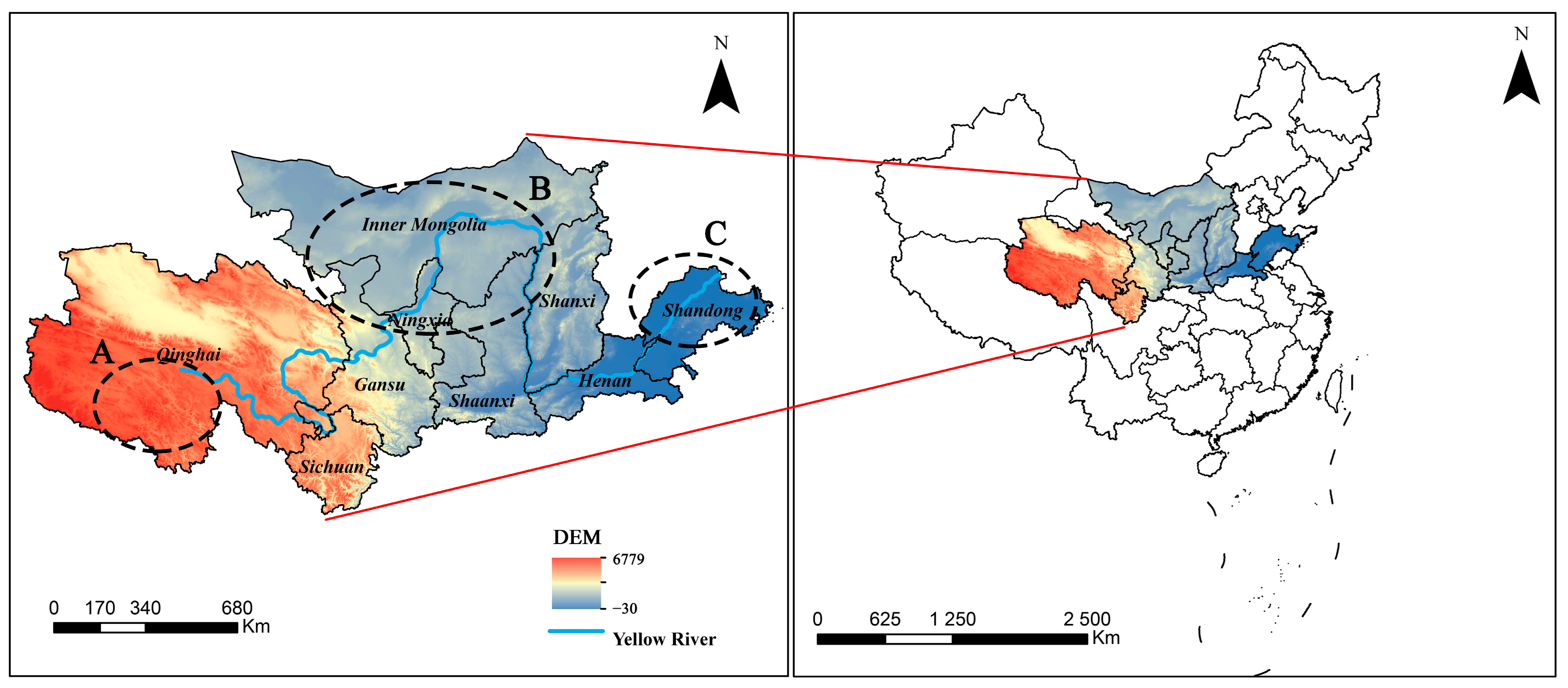
2.1. Study Area

2.1.1. Introduction to the Yellow River Basin

The Yellow River is the fifth largest river in the world and the second largest river in China [26]. The YRB (Yellow River Basin) belongs to the northern region of the East Asian monsoon region, which originates in Qinghai Province of China and passes through the Qinghai–Tibet Plateau, Inner Mongolia Plateau, Loess Plateau, and Yellow Huaihai Plain [27]. The Yellow River is 5464 km long and flows through nine provincial administrative regions (Figure 1). In recent years, the YRB has made great progress in the construction of ecological projects and ecological restoration, but different areas of the Yellow River Basin still face different ecological problems [25]. The three-river resource region is the birthplace of the Yellow River, which faces the problems of grassland degradation and soil erosion due to unreasonable human activities (Figure 1A) [28]. The middle and upper reaches of the Yellow River Basin flow through many desert areas (Mu Us Desert and Tengger Desert) and are facing serious land desertification and desertification problems (Figure 1B) [29]. The Yellow River Delta in the lower reaches of the YRB is the most complete wetland ecosystem in the warm temperate zone of China. but is currently facing problems of ecosystem degradation and biodiversity decline (Figure 1C) [30]. These ecological problems faced by the YRB hinder the development of the vegetation ecosystem and may affect the carbon sequestration process of vegetation [31]. Exploring the relationship between the topological characteristics of ecological nodes in the YRB and the carbon sequestration capacity of vegetation is a valuable reference for future national ecological project construction with the goal of carbon neutrality.

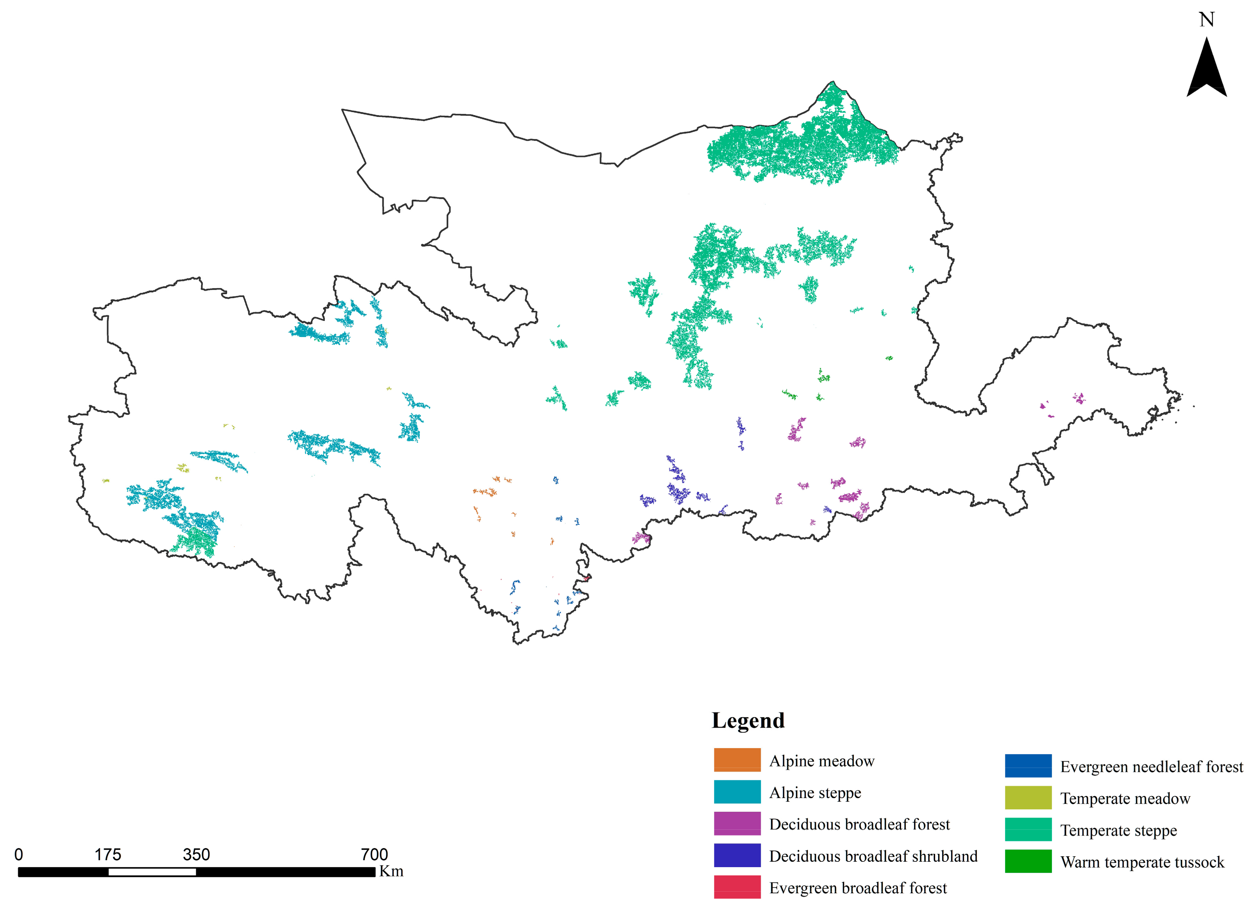
2.1.2. Vegetation Types in the Yellow River Basin

The vegetation types in the YRB include forests, shrublands, and grasslands [32]. Natural forests can be divided into deciduous broadleaf forests, evergreen needleleaf forests, evergreen broadleaf forests, and deciduous needleleaf forests according to the plant functional type. Among them, the deciduous broadleaf forest is the largest forest type in the YRB, with an area of 108,055 km². The deciduous broadleaf forests are mainly concentrated in Gansu, the southern region of Shaanxi, the south–central region of Shanxi, and the northwestern region of Henan. In addition, deciduous broadleaf forests have a fragmented distribution in Shandong and Inner Mongolia. Evergreen needleleaf forest is the second largest forest type in the YRB, with an area of 54,835 km², mainly represented in Sichuan, Shanxi, and the southwestern region of Gansu. Evergreen broadleaf forests and deciduous needleleaf forests have a smaller distribution area in the YRB. Evergreen broadleaf forests and deciduous needleleaf forests are scattered in the southern region of Sichuan and Shandong, respectively. The natural shrublands in the YRB are mainly deciduous broadleaf shrublands with an area of 221,115 km². The deciduous broadleaf shrublands are distributed in the central and southern regions of the YRB, concentrated in Gansu and Shanxi. The area of natural grasslands in the YRB is 864,352 km², which is much larger than the area of forests in the YRB. The main types of grassland are temperate meadow, temperate steppe, alpine steppe, alpine meadow, and tussock. The temperate steppe in the YRB has the largest area of 403,498 km², which is mainly distributed in Gansu, Ningxia, the southeastern region of Qinghai, the northern region of Shaanxi, and the southeastern region of Inner Mongolia. The area of alpine meadows and alpine steppes is relatively similar, with 159,960 km² and 157,888 km², respectively. Alpine meadows are mainly distributed in the southeastern region of Qinghai, while alpine steppes are mainly distributed in Sichuan, as well as the northern region of Qinghai. The area of tussock and temperate meadow is smaller, with 100,316 km² and 42,690 km², respectively. The tussocks are mainly gathered in Shanxi and Shaanxi, with less distribution in Gansu and Shandong. The temperate meadows are mainly distributed in the west–central and south–central region of Qinghai.

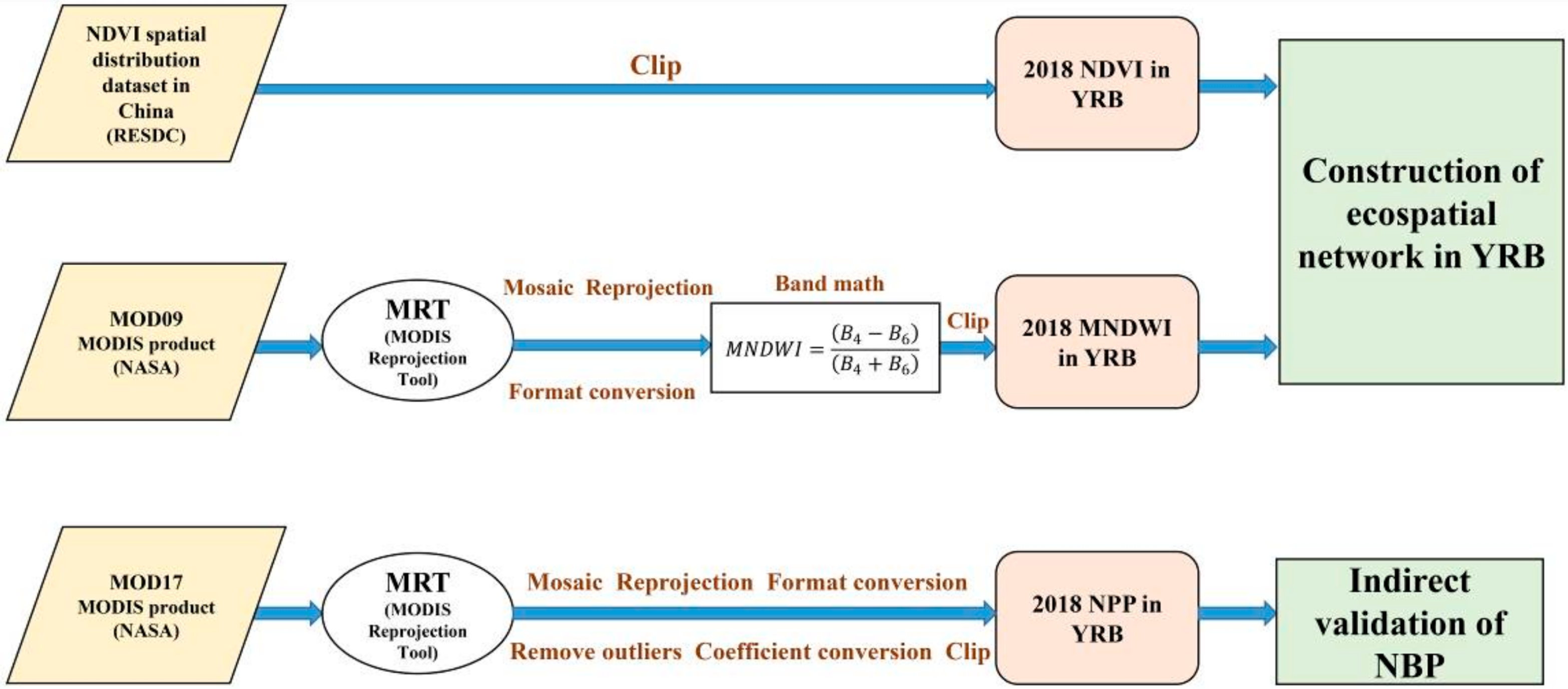
2.2. Data Sources and Processing of MODIS Products

2.2.1. Data Sources and Descriptions

The boundary of the study area comes from the extraction and cutting of the boundaries of 71 cities through which the Yellow River flows, and this operation was completed in ArcGIS 10.4. The study area was 3,207,084 km². The vegetation classification data in this study were obtained from the CNLUCC in 2018 (http://www.resdc.cn/DOI, accessed on 15 May 2021). With reference to the existing vegetation classification system, the vegetation distribution map of China, and the needs of the Biome-BGC model, we divided the vegetation types into nine categories, namely, deciduous broadleaf forest, evergreen broadleaf forest, evergreen needleleaf forest, deciduous broadleaf shrubland, warm temperate tussock, temperate steppe, temperate meadow, alpine meadow, and alpine steppe (http://westdc.westgis.ac.cn, accessed on 15 May 2021) [33]. The 2018 NDVI, topographic data (DEM, slope), and residential area distribution data used to construct the ecospatial network in this study were obtained from the Resource and Environmental Science and Data Center of the Chinese Academy of Sciences (https://www.resdc.cn/, accessed on 16 May 2021). MNDWI data were extracted from MODIS images with few clouds in summer 2018 (https://ladsweb.modaps.eosdis.nasa.gov/, accessed on 17 May 2021). Data on road network, water network, and railroad network were obtained through Overpass API (http://www.overpass-api.de/, accessed on 20 May 2021). Ecological sources comprise multiple ecological services that maintain ecosystem stability. Ecological sources are usually high-quality and representative landscape patches that are characterized by continuity and integrity [34]. When selecting ecological sources, fragmented and discontinuous patches are usually avoided. Combining the large area of the YRB (3,207,084 km²) in this study and avoiding fragmentation of the selected ecological sources, we chose 1 km as the resolution for each type of raster data.

The site geographic data required to drive the Biome-BGC model, including elevation, slope, and aspect, were extracted from the DEM data (https://www.resdc.cn/, accessed on 16 May 2021). The soil data required to drive the Biome-BGC model came from the spatial distribution data of soil texture in China (http://resdc.cn/, accessed on 16 May 2021). The CO₂ concentration data came from the annual average observation value of the Mauna Loa Observatory in the United States (https://www.co2.earth/, accessed on 18 May 2021). The daily meteorological data required by the Biome-BGC model needs to be simulated by inputting the original data of the meteorological observatory into the MTCLIM4.3 model (http://data.cma.cn; http://www.ntsg.umt.edu/project/mt-clim.php, accessed on 21 May 2021). The vegetation ecophysiological parameters required by the Biome-BGC model were all obtained by collecting reports in the literature.

2.2.2. Processing of MODIS Products

The three types of data needed in this study were from MODIS products, namely, NDVI, MNDWI, and NPP. NDVI and MNDWI were used for the construction of the ecospatial network of the YRB, while NPP was used for indirect validation of the NBP of vegetation nodes obtained from the Biome-BGC model simulations. The NDVI of the YRB was extracted from the spatial distribution dataset of NDVI at 1 km resolution for the growing season in China produced by the RESDC (Resource and Environmental Science and Data Center), which was verified to accurately reflect the cover status of surface vegetation. We clipped this data to obtain the 2018 NDVI of vegetation in the YRB.

The NPP was obtained from our processing of the MOD17 product from MODIS, which can be obtained from the open database of the National Aeronautics and Space Administration (NASA) [35]. This product provides annual NPP information at a 500 m pixel resolution. After we selected the row number where this study area was located, the obtained original product was mosaicked, reprojected, and data formatted by MRT (MODIS Reprojection Tool). After that, the invalid values (32,761 to 32,767) in the image of this product were set to null values. In addition, a coefficient conversion was performed on the remaining raster values. Multiplying the raster values by 0.1 produced the NPP units required for this study in g·C m⁻²·year⁻¹. Finally, the images were clipped using the extract by mask tool to obtain the 2018 annual NPP for the YRB required for this study.

The extraction of MNDWI for the YRB was from the MODIS MOD09 product, which includes atmospherically corrected surface reflectance data from the MODIS L1B product. Similar to the MOD17 product used for extracting the NPP, this product is also derived from NASA. We used the MRT (MODIS Reprojection Tool) to mosaic, reproject, and format the original product to extract surface reflectance data at a resolution of 500 m. This product has seven bands (B1 to B7). We obtained the MNDWI results by band math using the method proposed by Xu for calculating MNDWI [36]. The final MNDWI for 2018 in the YRB required for this study was obtained by clipping. The band calculation formula for MNDWI is

$$\mathrm{MNDWI}=\frac{\left(B_4-B_6\right)}{\left(B_4+B_6\right)},$$

(1)

where $B_4$ and $B_6$ represent the reflectance of the B4 and B6 bands of the MODIS product [37].

A flowchart is provided in Figure 2 representing the abovementioned processing of the MODIS product, the information extracted, and the subsequent usage.

2.3. Construction of Ecospatial Network

2.3.1. Introduction to Ecospatial Network

An ecospatial network is the application of complex network theory in landscape ecology. Many studies have reported on it, but no researchers have proposed the concept of an ecospatial network [22,38]. Here, we believe that the ecospatial network can be expressed as follows: in geographic space, a network that describes the topological relationship between different ecological objects. Ecological nodes are used to represent objects in space, which can have different ecological scales, such as individuals, populations, or ecosystems. Ecological corridors represent the relationship between objects and they have functions of information transmission, material circulation, and energy flow [39]. Corresponding to the concepts of vertices and edges in complex networks, the ecospatial network is composed of ecological nodes and ecological corridors [19]. In this study, the source of ecological nodes was the vegetation (forests, shrublands, and grasslands) of the YRB.

2.3.2. Identification of Ecological Sources

The construction of an ecospatial network usually includes two elements, ecological corridors and ecological nodes, whereby ecological nodes come from ecological sources [22]. Ecological sources comprise ecological services, which refer to patches that provide a variety of ecosystem services and have an important contribution to the development of the ecosystem [40]. In this study, the composition of the ecological source area constituted the vegetation patches (including forests, shrublands, and grasslands) in the YRB. By setting thresholds for patch area, patch perimeter, NDVI average, and patch shape index to identify ecological sources, patch area, patch perimeter, and NDVI average were calculated in ArcGIS 10.4. The patch shape index was calculated by Fragstats 4.2 (http://www.umass.edu/landeco/research/fragstats/fragstats.html, accessed on 20 May 2021). The entropy method was used to determine the weight of each index and comprehensively evaluate the importance of each patch [40].

2.3.3. Extraction of Ecological Corridors and Ecological Nodes

Ecological corridors are channels connecting ecological nodes in the ecospatial network, and they play an important role in the operation of ecological flows within the landscape [38]. There are many paths for the ecological flow in the landscape to start from the ecological source and reach another source through a resistant surface. The ecological corridor we constructed was the optimal path among many paths, i.e., the path of ecological flow with the least resistance [22]. The collection of all resistance factors that need to be overcome related to the flow from ecological sources to other sources is called the cumulative resistance surface [40]. The minimum cumulative resistance model (MCR model) can simulate and analyze the spatial operation mechanism of ecological flow and obtain the minimum cumulative resistance surface [20]. Afterward, the ecological corridor was obtained by combining the cost path model in ArcGIS 10.4. The MCR model was proposed by Kanppen, and it is widely used in corridor extraction for ecospatial networks [41]. The formula is

$$V_{MCR}=f_{min}{\displaystyle \sum }_{i=1,j=1}^{i=\mathrm{m}, j=n}\left(D_{ij}{R}_I\right),$$

(2)

where $V_{MCR}$ represents the value of the minimum cumulative resistance surface, $f_{min}$ represents the function of the minimum resistance value, $D_{ij}$ represents the spatial distance from the source to the landscape unit, and $R_I$ represents the coefficient of resistance in the process of source movement.

According to the habitat characteristics of vegetation in the YRB and other studies, we selected four types of resistance factors, namely, topographic and landform factors, vegetation coverage factors, hydrological factors, and density factors, to evaluate the resistance value of each patch in the study area (

Table 1. Ecological resistance factor evaluation system.

Resistance Type	Factor	Level	Ecological Resistance Value
Topography and landform	DEM	<1000 m	1
		1000–1500 m	3
		1500–3000 m	5
		3000–4500 m	7
		>4500 m	9
	Slope	0–2°	1
		2–5°	3
		5–8°	5
		8–14°	7
		>14°	9
Vegetation cover	NDVI	<0.2	9
		0.2–0.4	7
		0.4–0.6	5
		0.6–0.8	3
		>0.8	1
Hydrology	MNDWI	<0.05	9
		−0.05–0.02	7
		−0.02–0.02	5
		0.02–0.08	3
		>0.08	1
Density	Residential density	0–0.08	1
		0.08–0.24	3
		0.24–0.44	5
		0.44–0.66	7
		>0.66	9
	Road network	0–0.02	1
	Density	0.02–0.06	3
		0.06–0.1	5
		0.1–0.16	7
		>0.16	9
	Water network	<0.17	9
	Density	0.17–0.43	7
		0.43–0.84	5
		0.84–1.53	3
		>1.53	1
	Railway network density	<0.003	1
		0.003–0.01	3
		0.01–0.02	5
		0.02–0.04	7
		>0.04	9

) [40,42]. In the process of abstracting the ecological space to the complex network, the ecological source was abstracted as multiple nodes in the network. Ecological nodes come from ecological sources and represent the habitat characteristics of ecological sources to a large extent [20]. We extracted the centroid of the ecological source and then selected the point on the ecological corridor closest to the centroid as the ecological node [40].

2.4. Algorithm for Topological Indicators

According to the theoretical foundation of complex networks and graph theory, there are many topological indicators used to describe the topological characteristics of ecospatial networks [17]. These indicators are divided into those used to evaluate the topological characteristics of ecological nodes and those used to evaluate the ecospatial network as a whole. Combining the ecological significance of each topological indicator and the selection of topological indicators in other studies of ecospatial networks, we selected 10 topological indicators to evaluate the ecospatial network of the Yellow River Basin [21,40]. Among them, six topological indicators were used to evaluate the ecological nodes, and four topological indicators were used to evaluate the network as a whole (

Table 2. Description of the 10 topological indicators.

Type of Indicator	Name of Indicator	Introduction to the Algorithm	Significance of Indicator	Reference
Evaluation of nodes	Degree	The number of ecological corridors owned by an ecological node	Describes the number of connections between an ecological node and other ecological nodes	[17]
	Clustering coefficient	The ratio of the number of corridors actually existing between the neighboring nodes of a node to the maximum number of corridors that may exist	Indicates the proportion of connectivity between neighboring nodes of an ecological node	[17]
	Closeness centrality	The reciprocal of the sum of the shortest distances from a node to all other nodes multiplied by the number of other nodes	Indicates how close the ecological node is to other nodes through the shortest path; at the same time, it also quantifies how much the ecological node is in the geometric center of the network	[43]
	Betweenness centrality	The normalized index of the proportion of all the shortest paths in the network that pass through a node	Indicates the proportion or degree to which an ecological node exists on the shortest path of any two nodes in the network	[17]
	Eigenvector centrality	Each ecological node is assigned a relative score; connections to nodes with high scores are weighted more than connections to nodes with low scores	The more important the node connected to node A, then the more important node A is; this indicator is used to evaluate the importance of nodes	[43]
	PageRank	Rank of the importance of ecological nodes, evolved from eigenvector centrality	Similar to eigenvector centrality, it is an indicator used to evaluate the importance of nodes	[44]
Evaluation of the network	Average degree	Average of the degrees of all ecological nodes in the network	Evaluates the average connectivity of all nodes in the network	[17]
	Average path length	Average of the shortest distance between any two ecological nodes in the network	Indicates the smoothness of energy flow of the whole ecospatial network	[17]
	Average clustering coefficient	Average of the clustering coefficients of all nodes in the network	Indicates whether the distribution of ecological nodes in the network tends to be concentrated or decentralized	[17]
	Modularity	Each ecological node in the network is assigned to a different community	Evaluates the effect of network community division	[45]

). After calculating the results of the topological indicators, six indicators for evaluating ecological nodes were used to establish relationships with each node’s NBP in 2018, while the remaining four topological indicators were used to evaluate the current status of the ecospatial network of vegetation in the YRB. We describe these 10 indicators in detail with a brief introduction, the significance of indicators, and references in Table 2. Moreover, the formulas for calculating these indicators are described in the Supplementary Materials (Text S1). In addition, we express three concepts here as a supplement to Table 2: the shortest path of a node is the path in the network that passes through the minimum number of corridors from one node to another; the distance is defined as the number of corridors contained in the shortest path connecting two nodes; the diameter of the network is the maximum value of the distance between any two ecological nodes [17].

2.5. Evaluation of the Indicator of Carbon Sequestration Ability

In this study, the ecological nodes represent the vegetation ecosystems in their locations. Researchers usually use GPP or NPP to express the carbon sequestration capacity of vegetation. GPP represents the ability of green plants to fix CO₂ from the atmosphere through photosynthesis, while NPP is GPP minus the part consumed by autotrophic respiration [46]. In forest or grassland ecosystems as a whole, the amount of CO₂ excreted through soil respiration may be higher than that fixed by green plants. In addition, the carbon changes caused by external disturbances (e.g., forest fires) to the ecosystem need to be considered. Therefore, we believe that NBP (net biome productivity) better reflects the overall net carbon sequestration capacity of vegetated ecosystems [47]. The calculation formula of NBP is

$$NBP=GPP-Ra-Rh-NR,$$

(3)

where $GPP$ represents the gross primary productivity, $Ra$ represents the autotrophic respiration consumption, $Rh$ is the heterotrophic respiration consumption (soil respiration), and $NR$ is the photosynthetic product consumed by non-respiratory metabolism.

NBP is a vegetation productivity concept applied at the landscape scale, and its unit is g·C m⁻²·year⁻¹, with positive or negative values. Actually, NBP is numerically the value of carbon sources or sinks in terrestrial ecosystems in global change studies. A positive NBP value indicates that the vegetation ecosystem as a whole is a carbon sink, fixing more carbon per unit time than it emits. Conversely, a negative NBP value indicates that the ecosystem as a whole is a carbon source, fixing less carbon per unit time than it emits. The magnitude of the absolute value of the NBP value indicates the strength of the net sequestration or emission of CO₂ by the vegetated ecosystem, i.e., the strength of the carbon sequestration capacity [46].

2.6. Biome-BGC Model and Its Validation

2.6.1. Description of the Biome-BGC Model

The Biome-BGC model is a classic biogeochemical cycle model. Because of its true description of the carbon cycle, nitrogen cycle, and water cycle of the ecosystem, it is widely used in ecological research [48]. At present, the Biome-BGC model is still a powerful tool for many researchers to conduct large-scale ecological research, and many studies have reported that it has a good simulation effect in most areas of the world [49,50,51]. The latest version of the Biome-BGC model is 4.2 (http://www.ntsg.umt.edu/project/biome-bgc.php, accessed on 5 May 2021). The input data of the Biome-BGC model consists of three parts: geographic data, meteorological data, and ecophysiological parameters of vegetation. Through detailed calculation of the biogeochemical process of the ecosystem, a number of vegetation productivity results can be finally obtained, including GPP, NPP, and NBP [48]. In this study, we parameterized the ecophysiological parameters of each node representing the vegetation ecosystem. The ecophysiological parameters came from our review of the literature. If there was no report in the literature, the default parameters of the plant functional type to which the node belongs were used. This study used the parameterized Biome-BGC model to simulate the annual NBP of all ecological nodes in the YRB from 2009 to 2018.

2.6.2. Indirect Validation of the Biome-BGC Model

The NPP product of MODIS has been used by many researchers, and many studies have reported on its accuracy and reliability [52,53]. Researchers often use MODIS NPP products to directly validate the accuracy of NPP simulated by the Biome-BGC model [54]. In this study, NBP was selected as the output of the Biome-BGC model in order to explore the relationship between the topological characteristics of vegetation and its net carbon sequestration capacity in the YRB. However, there are hardly any spatially available data and products that can directly validate the NBP of vegetation ecosystems. The values of NPP are different from those of NBP, and its direct validation of NBP is not possible. However, NPP and NBP have large overlapping processes in their calculations, and they both describe two important mechanistic processes in vegetated ecosystems: photosynthesis and autotrophic respiration. Furthermore, the focus of this study was to explore the relationship between the spatial topology of vegetation nodes and their net carbon sequestration capacity. We put more emphasis on the reliability of the Biome-BGC model in simulating the spatial heterogeneity of productivity of different vegetation nodes. Therefore, we chose MODIS NPP as an indirect validation product of the NBP simulated by the Biome-BGC model. The objective of the indirect validation was to determine if the spatial variability trends of NBP at different vegetation nodes were close to the spatial variability trends of NPP at these nodes. We compared these two productivity results in a dual Y-axis coordinate system to see if the trends in variability of these two productivity results at different nodes were similar and to determine if this similarity was statistically significant through correlation analysis. The resolution of the NPP product of MODIS is 500 m, which was sufficient for the 1 km resolution ecological source of this study. We extracted NPP values for all vegetation nodes from the MODIS NPP products and used correlation analysis to determine the correlation between NPP and NBP. The above operations were finished in ARCGIS 10.4 and SPSS 24.0.

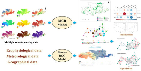
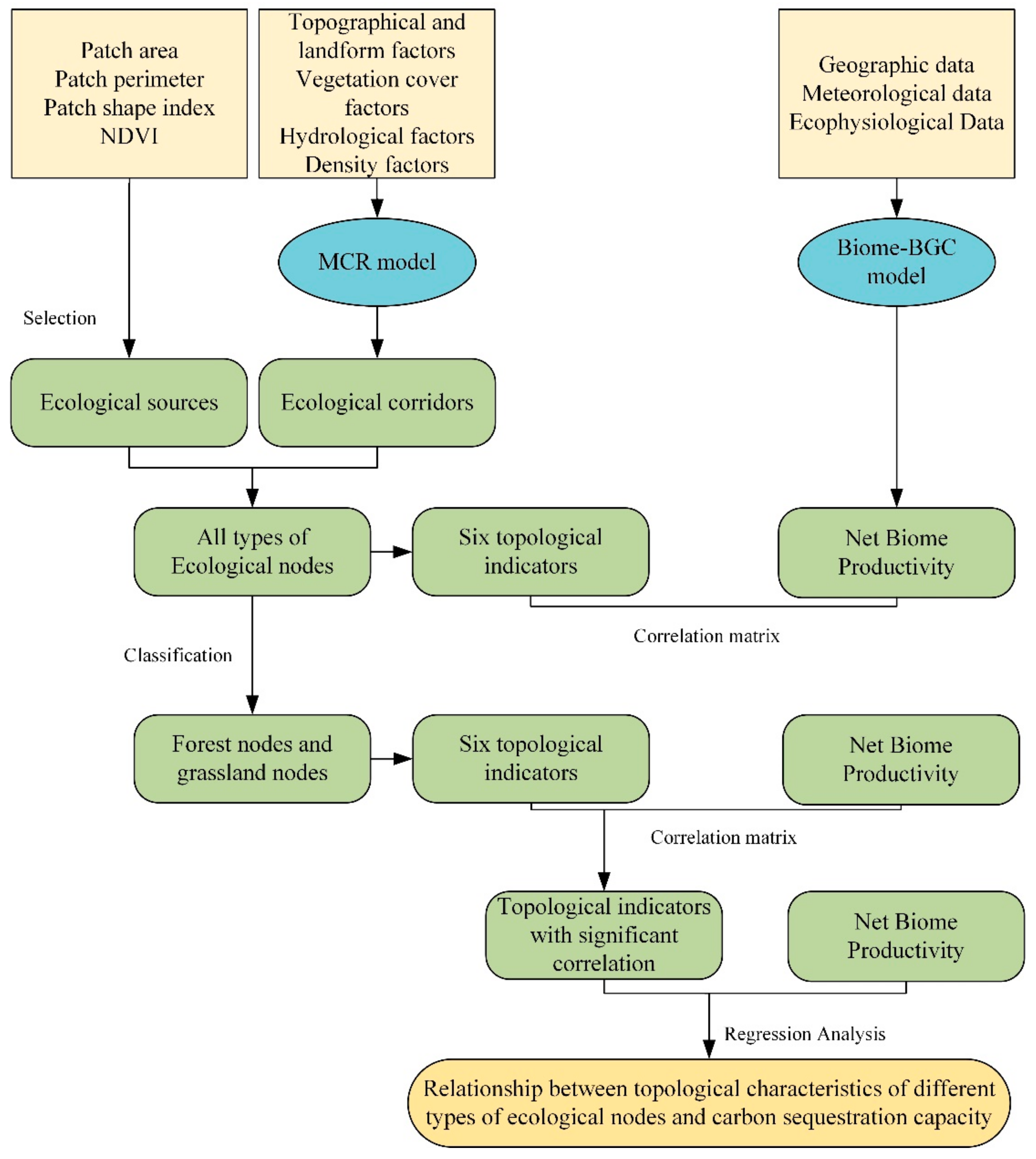
2.7. Statistical Analysis and Technical Routes

In this study, correlation matrices and regression analyses were used to explore the relationship between the topological characteristics of ecological nodes and the carbon sequestration capacity (NBP) of the vegetation ecosystem in which the nodes are located. First, we calculated the Pearson’s correlation coefficient between the six topological indicators (degree, clustering coefficient, closeness centrality, betweenness centrality, eigenvector centrality, and PageRank) of ecological nodes of all vegetation types and their NBP in 2018 by constructing a correlation matrix. We considered the possible influence of plant functional types (forest or grass) on the relationship between topological indicators and NBP. Therefore, we divided the ecological nodes into forest nodes (including shrubland nodes) and grassland nodes according to vegetation type, and then separately calculated the Pearson’s correlation coefficients between the topological indicators and the NBP in 2018. Finally, we screened out the topological indicators with significant correlations for linear regression analysis with NBP to determine the relationship between topological indicators and NBP. The above statistical analysis was done in R studio. For a clear and coherent representation of the methodology and data analysis of this study, a schematic diagram of the study framework is shown in Figure 3.

3. Results

3.1. Results of Factors for Constructing Ecospatial Networks

We present the results of the eight factors used to construct the ecospatial network and the NPP used to indirectly validate the Biome-BGC model in Figure 4. The first three factors (NDVI, MNDWI, and NPP) were extracted from MODIS products, where the unit of NPP is g·C m⁻²·year⁻¹ and NDVI and MNDWI are dimensionless. The distribution of NDVI in the YRB ranged from 0 to 0.92, and its value showed a gradual increasing trend from northwest to southeast. The distribution of MNDWI in the YRB ranged from −0.72 to 0.96, and the dark-blue part of the figure is the water body (Figure 4 MNDWI). The results of MNDWI show that the water bodies were more distributed in the western region of the YRB than in other regions. The NPP results were white in the northwestern region of the YRB because the NPP products of MODIS were filled with invalid values in these areas. These invalid values represent the non-vegetated land-cover type in these regions [35]. With the same trend as NDVI, NPP in the YRB showed a gradual increase from northwest to southeast. The slope of the YRB was extracted from DEM, and this operation was implemented by the 3D Analyst tool in ARCGIS 10.4. The DEM and slope results of the YRB show that the western region of the Yellow River Basin was at a higher elevation than the other regions, and the topography in the west was more complex than the other regions. The remaining four results of density analysis were involved in constructing the cumulative resistance surface of the YRB. From these density results, it can be seen that the southeastern region of the YRB had more human activities than the other regions. This also implied that the vegetation in the southeastern region of the YRB may be more disturbed by humans than other areas.

3.2. The Construction Process and Results of Vegetation Ecospatial Network in the YRB

3.2.1. Extraction of Ecological Sources

The ecological sources of the YRB we extracted included nine types of vegetation and a total of 554 vegetation patches. The total area of ecological sources was 189,512 km², accounting for 5.9% of the study area (Figure 5). Among the ecological sources, temperate steppe had the largest number of patches at 202, and evergreen broadleaf forest had the least number of patches at 14. The vegetation type that accounted for the largest area of ecological sources was temperate steppe, and the smallest area was evergreen broadleaf forest. In terms of spatial distribution, the proportion of grassland patches in ecological sources was much larger than that of forest patches. Grassland patches were mostly distributed in the northern and western regions of the YRB, and forest patches were mostly distributed in the southern and eastern regions.

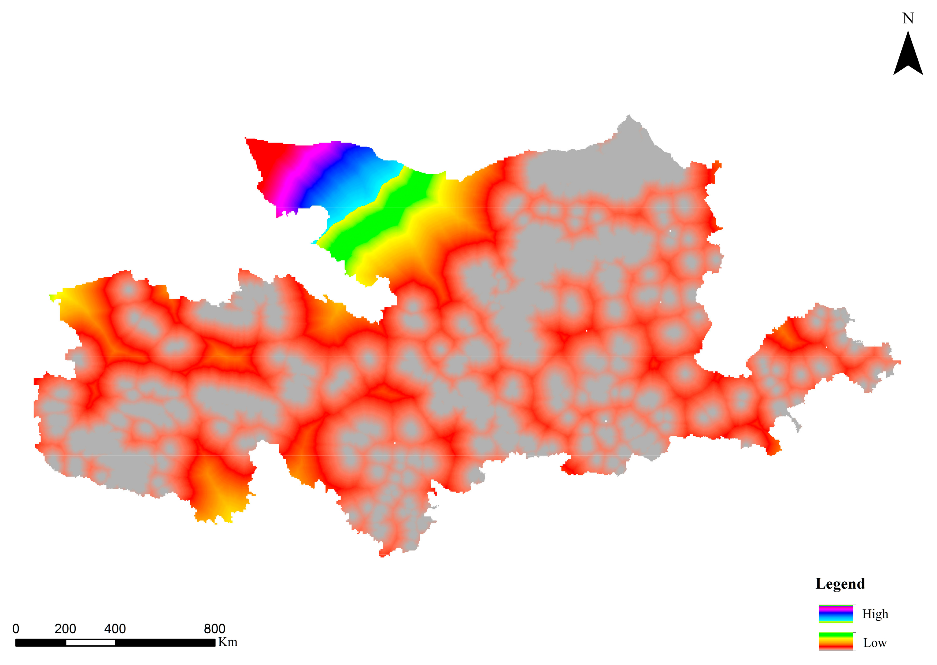
3.2.2. Results of Cumulative Resistance Surface

According to the ecological resistance factor evaluation system in Table 1, the results of the minimum cumulative resistance surface constructed using the MCR model are shown in Figure 6. It can be seen that the resistance value in the northwestern region of Inner Mongolia gradually increased, reaching the highest value in the western region of Inner Mongolia, which is the fourth largest desert in China, the Tengger Desert. The reason for this result is that the ecological environment in this region was in poor condition, and the resistance values of several factors, such as NDVI, MNDWI, and water density, were high. In addition, the vegetation patches in this area were less distributed and were far away from the existing ecological sources, which caused a significant accumulation of ecological resistance.

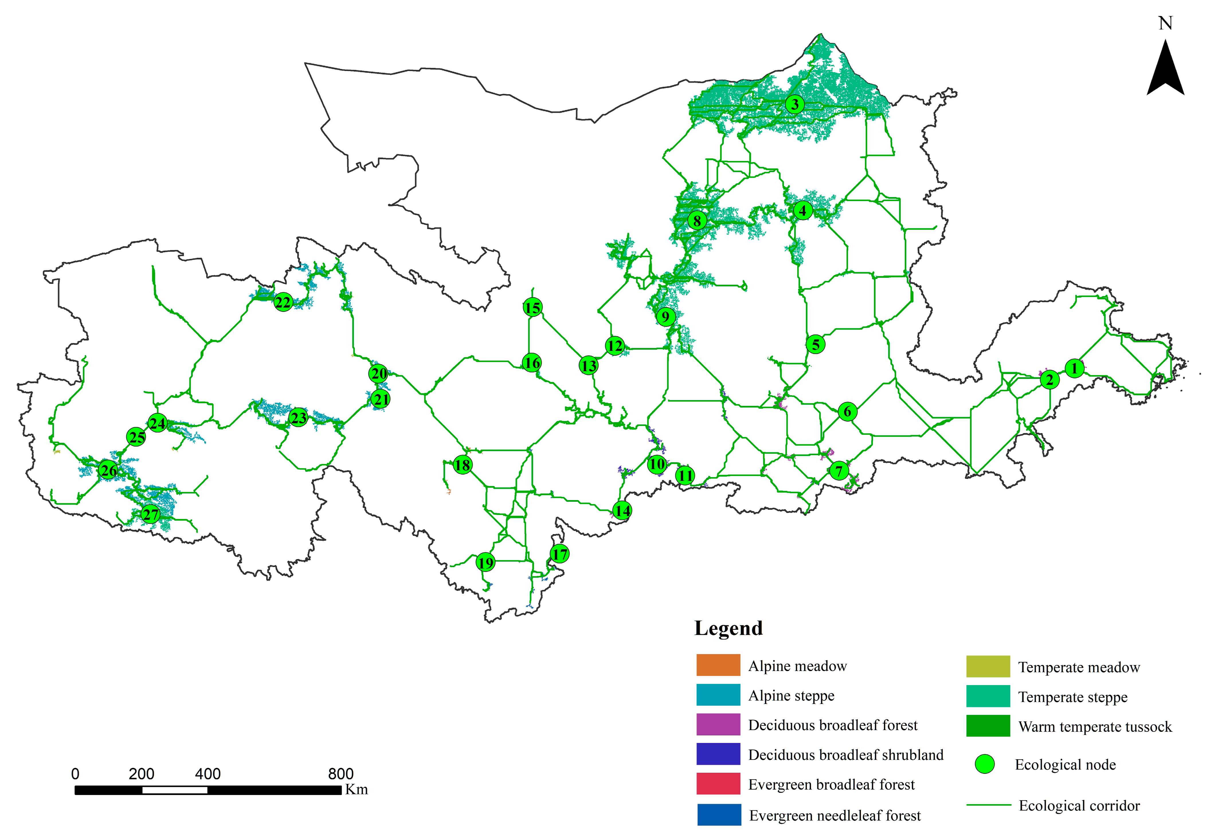
3.2.3. Construction of Vegetation Ecospatial Network in the YRB

Combined with the results of cumulative resistance surface above, we extracted ecological corridors using the cost path model. Then, we extracted ecological nodes in combination with ecological sources and finally constructed the vegetation ecospatial network of the YRB (Figure 7). The network contained a total of 27 ecological nodes and 84 ecological corridors, and the ecological nodes represented different vegetation ecosystems. We numbered the 27 ecological nodes according to their geographical locations and counted the plant function type, latitude and longitude, and province information represented by each node (Table S1). It can be seen that Qinghai Province, located in the westernmost part of the network, had the largest number of ecological nodes, while the central and eastern provinces had fewer ecological nodes. In addition, the number of ecological nodes was closely related to the distribution of ecological sources and ecological corridors. There were fewer ecological sources in the central–eastern region of the YRB, which led to a small number of ecological nodes.

3.3. Results of Topological Indicators

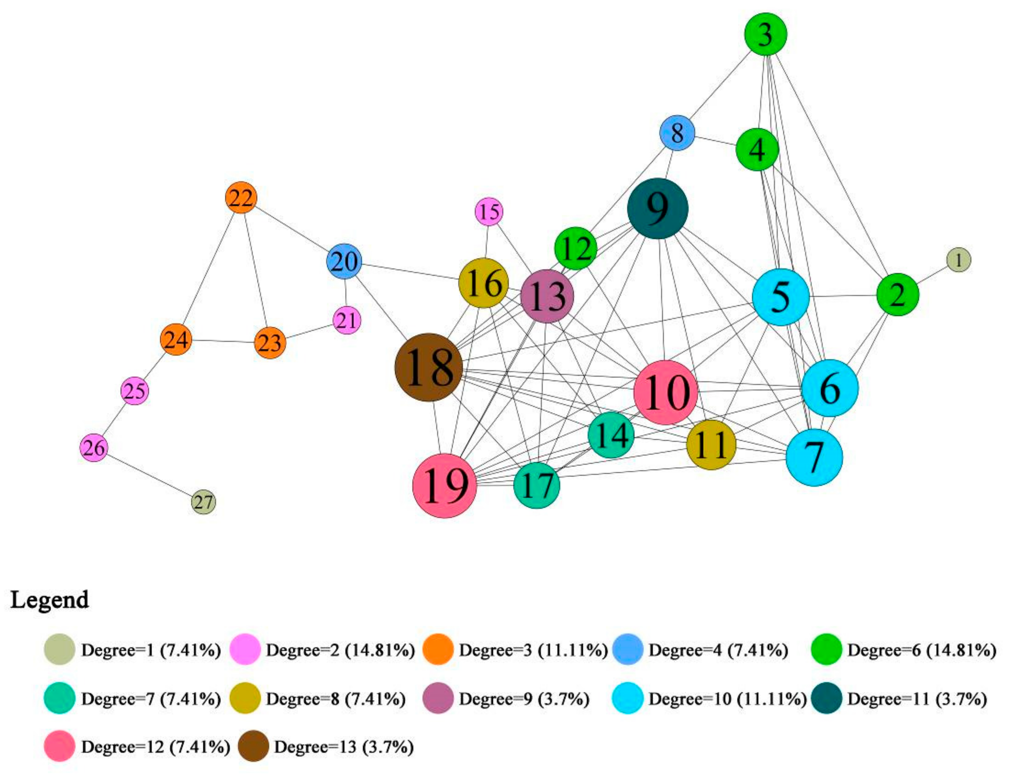
3.3.1. Results of the Topological Indicators Describing the Ecological Nodes

The degree of an ecological node indicates the number of ecological corridors it is connected to. In order to more clearly represent the difference in degrees between nodes, we present the results of degrees in the network (Figure 8). The remaining topological indicators of the ecological nodes had values between 0 and 1, as presented in Figure 9. Node 18 had a degree of 13 and was the node with the largest degree. On the other hand, Node 1 and Node 27, which were at the edge of the network, both had a degree of 1 and were the nodes with the smallest degree. In an ecological context, the degree describes the connectivity between ecological nodes. Node 18 was the alpine meadow located in Qinghai province, which had the highest connectivity in this network. According to its degree, Node 18 had an important position in the network. Node 1 and Node 27 were deciduous broadleaf forest and temperate steppe located in Shandong and Qinghai, and they had the lowest connectivity in the network.

The clustering coefficient reflects the proportion of connections between the neighboring nodes of the ecological nodes. Node 15 was the node with the largest clustering coefficient in the ecospatial network, and its clustering coefficient was 1. This indicated that all neighboring nodes around Node 15 were connected to each other. Node 21, Node 25, Node 26, and Node 27 were the four ecological nodes with a clustering coefficient of 0. This showed that none of their neighboring nodes were connected to each other.

Closeness centrality describes the shortest path from a node to all other nodes: the higher the closeness centrality, the more the node is located at the topological center of the network. In this study, the node with the highest closeness centrality was Node 18 and the node with the lowest closeness centrality was Node 27, which means that Node 18 was at the topological center of the network and Node 27 was at the topological edge of the network.

Betweenness centrality describes the proportion of a node that is located between any two nodes in a network. Nodes with high betweenness centrality play the role of a “bridge” in the ecospatial network. In this study, the node with the highest betweenness centrality was Node 20, and the node with the lowest betweenness centrality was Node 27. Thus, if Node 20 is lost, all nodes with a number greater than 20 would be disconnected from the main body of the network (Figure 8). Therefore, Node 20 represented the “stepping stone” of the ecospatial network.

The core purpose of eigenvector centrality is to evaluate a node by the number and importance of its neighboring nodes, and it is a comprehensive indicator to measure the transmission effect and connectivity between nodes. Ecological nodes with high eigenvector centrality are usually surrounded by neighboring nodes that also occupy an important position in ecospatial network. Similar to the results of closeness centrality, the nodes with the highest and lowest eigenvector centrality in this study were still Node 18 and Node 27. PageRank is a variant of the eigenvector centrality, and the difference between them is the algorithm for the weight of important nodes. The node with the highest PageRank was still Node 18, while the node with the lowest PageRank was Node 1. It is not difficult to find that the results of the above different topological indicators overlapped. For example, Node 18 was evaluated as the most important node by multiple indicators.

3.3.2. Results of the Topological Indicators Describing the Network

The average degree of the vegetation ecospatial network in the YRB was 6.22, which means that each ecological node in the network had an average of 6.22 corridors. On the other hand, the diameter of the network was 9, the average path length was 3.014, and the average clustering coefficient of the network was 0.547. The clustering coefficients of the network in this study were larger compared with other studies, which indicated that the aggregation of the network in this study was relatively good, and the distribution of some ecological nodes was more concentrated [55]. In addition, the small average path length and the large average clustering coefficient indicate that the ecospatial network constructed in this study had the characteristics of a small world. The small-world characteristics of complex networks are closely related to the information dissemination in the network. In small-world networks, information transmission is fast, and the performance of the network can be greatly improved with a small change of a few connections [56,57]. This showed that the ecospatial network of the YRB has great potential for optimization in the future.

Through the community division algorithm, the ecospatial network was divided into three communities (Figure 10). Different communities contained different numbers of nodes. Community 1 had the largest number of nodes, which was 12. Community 2 contained eight nodes, and Community 3 contained seven nodes. We usually consider networks to have a distinct community structure when their modularity is between 0.3 and 0.7 [58]. The modularity of the network in this study was calculated to be 0.327, which is a good result for community division. Combining the results of the clustering coefficient of the nodes, we found that the nodes with higher clustering coefficients were all in Community 1 (Figure 9 and Figure 10). The clustering coefficients of nodes were significantly stratified across communities, and the average clustering coefficients of nodes in Community 1 were larger than those in Community 2 and Community 3.

3.4. NBP Simulation Results and Validation

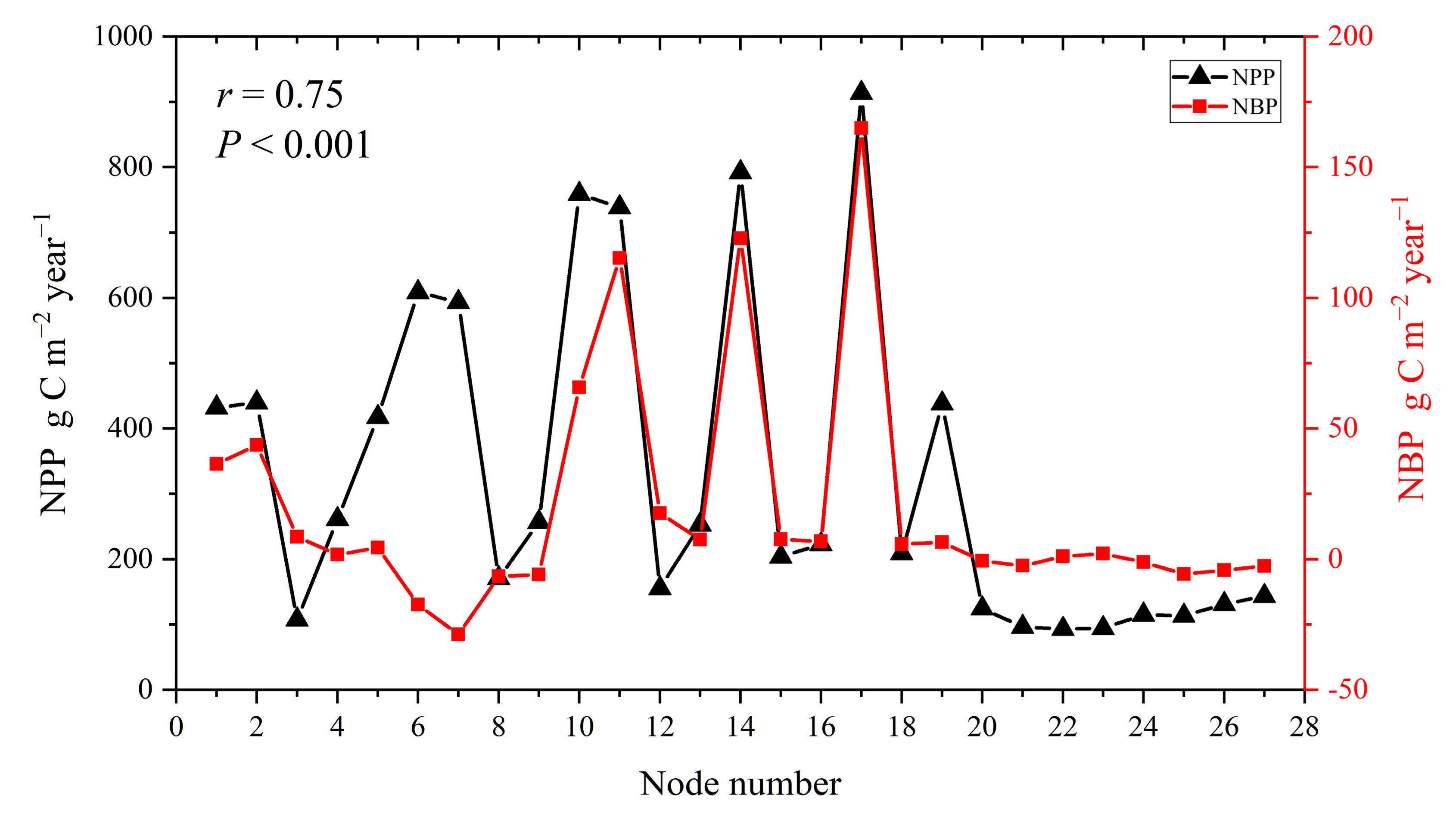
3.4.1. NBP Simulation Results for Ecological Nodes

We used the parameterized Biome-BGC model to simulate the annual average NBP of vegetation ecosystems in 27 ecological nodes of the YRB during 2009–2018, with the complete results for 10 years presented in Table S2 and the results for only 2018 presented in Figure 11. On a temporal scale, the ecological nodes of the YRB were in a state of alternating carbon sources and sinks from 2009–2018. Some nodes were in a state of gradually increasing carbon sink intensity in recent years, such as Node 2. Node 2 represented the deciduous broadleaf forest located in Shandong, whose annual NBP was −4.2 g·C m⁻²·year⁻¹ in 2014 and 5.6 g·C m⁻²·year⁻¹ in 2015. During this period, the NBP of Node 2 increased by about 233%, which means that Node 2 changed from a carbon source to a carbon sink in 2015. Between 2015 and 2018, Node 2’s NBP increased from 5.6 g·C m⁻²·year⁻¹ to 43.7 g·C m⁻²·year⁻¹, an increase of about 680%. Similar to Node 2 was Node 17, whose annual NBP increased from 15.7 g·C m⁻²·year⁻¹ to 165 g·C m⁻²·year⁻¹ between 2015 and 2018, an increase of about 950%, which implied a significant increase in the carbon sequestration capacity of Node 17 during that period. Similarly, some nodes were in carbon sink status in recent years but converted to a carbon source in 2018, such as Node 27. Node 27 represented the temperate steppe in Qinghai, which was in carbon sink status in 2014 (NBP of Node 27 in 2014 was 0.6 g·C m⁻²·year⁻¹) but converted to a carbon source in 2018 (NBP of Node 27 in 2018 was −2.6 g·C m⁻²·year⁻¹). The NBP of Node 27 in 2018 was 533% lower than in 2014. In addition, some nodes were carbon sources in recent years, such as Node 7. Node 7 was the deciduous broadleaf forest located in Henan, which was a carbon source between 2016 and 2018. The NBP of Node 7 increased by about 38.5% in 2018 compared to 2016. We speculate that the transformation of these vegetation nodes in the state of carbon sources or carbon sinks is the result of climate change, construction of national ecological projects, human management, and other factors.

In the 2018 NBP results, 17 ecological nodes were in carbon sink status and 10 ecological nodes were in carbon source status (Figure 11). The node with the largest carbon sink intensity was Node 17, with an annual NBP of 165 g·C m⁻²·year⁻¹. This node represented evergreen broadleaf forest located in Sichuan, which had the strongest net carbon sequestration capacity in the ecospatial network in 2018. The node with the largest carbon source intensity was Node 7 with an annual NBP of 28.8 g·C m⁻²·year⁻¹. Node 7 represented the deciduous broadleaf forest located in Henan, which was the node with the strongest net carbon emission capacity in the ecospatial network in 2018. In addition, some carbon source nodes (Node 24, 25, 26, and 27) had a small aggregation in the western region of Qinghai, which is the focus of future national ecological project construction in the context of carbon neutrality (Figure 11, far left). In terms of vegetation types of nodes, forest nodes had much higher intensity of net carbon sequestration or net carbon emission per unit time than grassland nodes. In addition, the total and mean values of NBP of carbon sink nodes in the YRB were much larger than those of carbon source nodes.

3.4.2. Results of Indirect Validation of NBP

The comparison of the NBP and NPP results for all vegetation nodes in 2018 is shown in Figure 12. The black triangles and the left y-axis in the figure indicate the NPP results of vegetation nodes (extracted from MODIS), and the red squares and the right y-axis indicate the NBP results of vegetation nodes (simulated from the Biome-BGC model). The results of NBP and NPP for all vegetation nodes showed a significant correlation (r = 0.75, p < 0.001; Figure 12). In addition, it can be seen from Figure 12 that the trend of NBP at different vegetation nodes simulated by the Biome-BGC model was closer to that of NPP products from MODIS at different vegetation nodes. This indicates that the Biome-BGC model can better simulate the spatial variation pattern of productivity of vegetation nodes in the YRB.

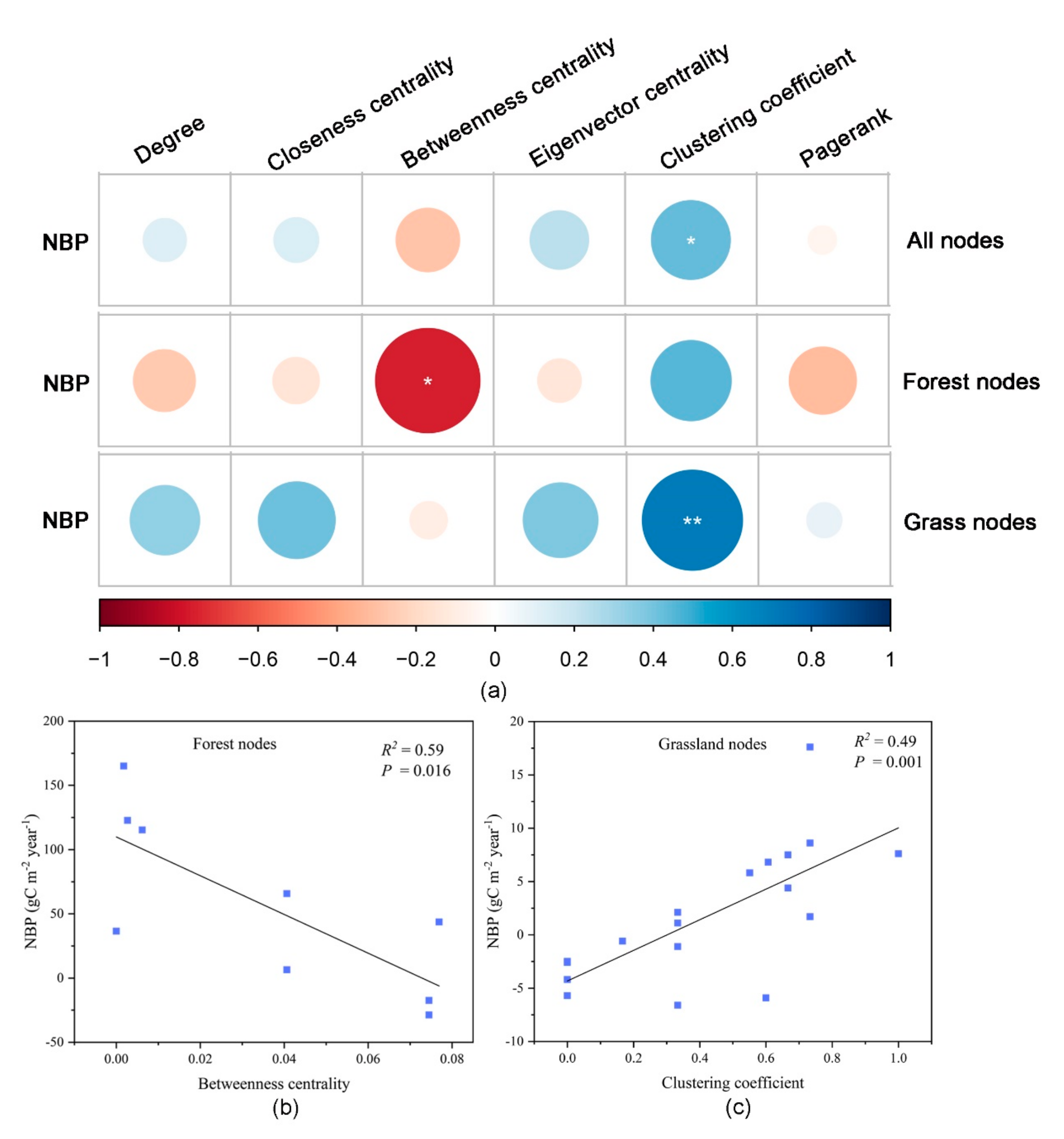
3.5. Relationship between Topological Indicators and Carbon Sequestration Capacity of Ecological Nodes

The results of the correlation matrix between topological indicators and NBP for ecological nodes of all vegetation types showed that only the clustering coefficients were significantly correlated with NBP (p < 0.05, Figure 13a). However, even at a larger regional scale, we believe that the plant functional types are still the decisive factor in productivity. Therefore, the results of the correlation matrix after the ecological nodes were divided into forest nodes and grassland nodes according to vegetation type showed that the betweenness centrality of forest nodes was significantly correlated with NBP (p < 0.05), and the clustering coefficient of grassland nodes was significantly correlated with NBP (p < 0.01, Figure 13a). The results of the subsequent linear regression analysis showed that the betweenness centrality of forest nodes showed a negative linear correlation with NBP (R² = 0.59, p < 0.05; Figure 13b), and the clustering coefficient of grassland nodes showed a positive linear correlation with NBP (R² = 0.49, p < 0.01; Figure 13c).

Betweenness centrality describes the proportion of ecological nodes present on the shortest path of any two nodes in the network, and it measures the intermediary properties of ecological nodes. Some studies refer to nodes (regions) with high betweenness properties as “stepping stones” [38]. For the forest nodes in the YRB, as the betweenness centrality increased, the NBP decreased linearly. In the process of decreasing NBP, a value of 0 represented the cutoff point for the forest node being in the state of carbon source or carbon sink. In other words, as the net carbon sequestration capacity of the forest ecosystem decreases, the carbon sink node will be transformed into a carbon source node. The clustering coefficient reflects the proportion of connectivity between neighboring nodes around a node. For the grassland nodes in the YRB, the NBP gradually increased as the clustering coefficient increased. This means that the net carbon sequestration capacity of the grassland ecosystem will gradually increase, and the carbon source will be transformed into a carbon sink.

4. Discussions

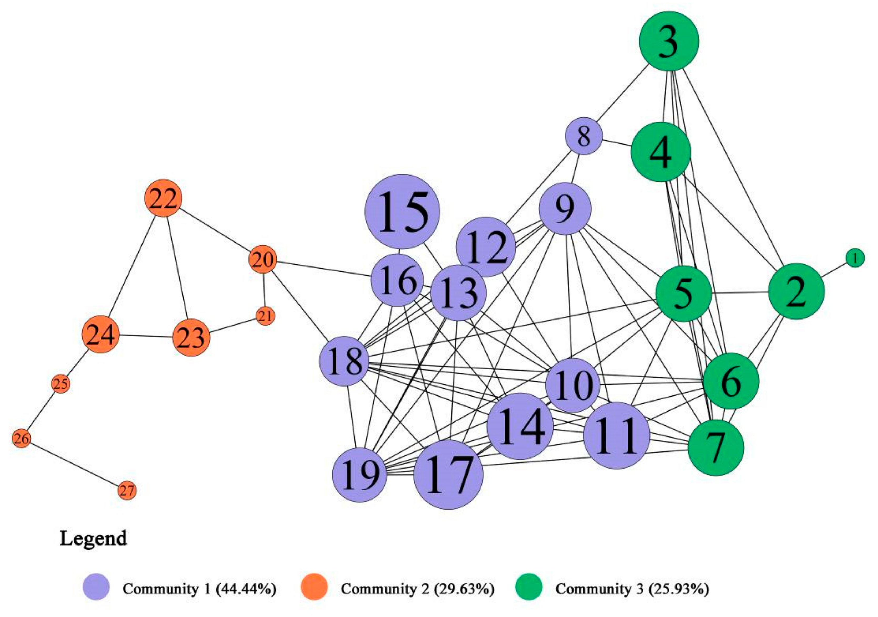
4.1. Community Division and Aggregation of Nodes

The vegetation ecospatial network of the YRB was divided into three communities (Figure 10). Combining the results of community division with the topological indicators of ecological nodes, we found that nodes with high topological indicators were mostly distributed in Community 1, while nodes with low topological indicators were more distributed in Community 2. For example, Node 18, Node 10, and Node 17, which were the top two in several topological indicators, were all located in Community 1. Meanwhile, Node 27 and Node 26, which ranked in the bottom two positions in several topological indicators, were located in Community 2 (Figure 10 and Table S3). From the perspective of network topology and landscape ecology, nodes with larger topological indicators contribute more to the network and are of higher importance. On the other hand, nodes with smaller topological indicators are in a weak position in the network and need to be focused on [40]. Interestingly, similar to the aggregation of nodes in different communities based on topological indicators, nodes also had aggregation in different communities according to the division of carbon sources or carbon sinks. The carbon sink nodes in 2018 were more concentrated in Community 1, while the carbon source nodes appeared to be clustered in Community 2 (Figure 10 and Figure 11). As proposed by the second law of geography (spatial segregation creates heterogeneity among ground objects [59]), we believe that it was the spatial heterogeneity that caused the differences between the topological indicators of ecological nodes in different communities, as well as caused the aggregation of carbon source and carbon sink nodes in different communities. This may also confirm the point we made in the introduction that the carbon sequestration capacity of vegetation nodes is related to their topological characteristics. In addition, it is obvious that the western part of the vegetation ecospatial network in the YRB is a weak area where the vegetation carbon sequestration capacity needs to be increased through the construction of national ecological projects. This is also consistent with the findings of previous studies on the vegetation cover of the YRB [42].

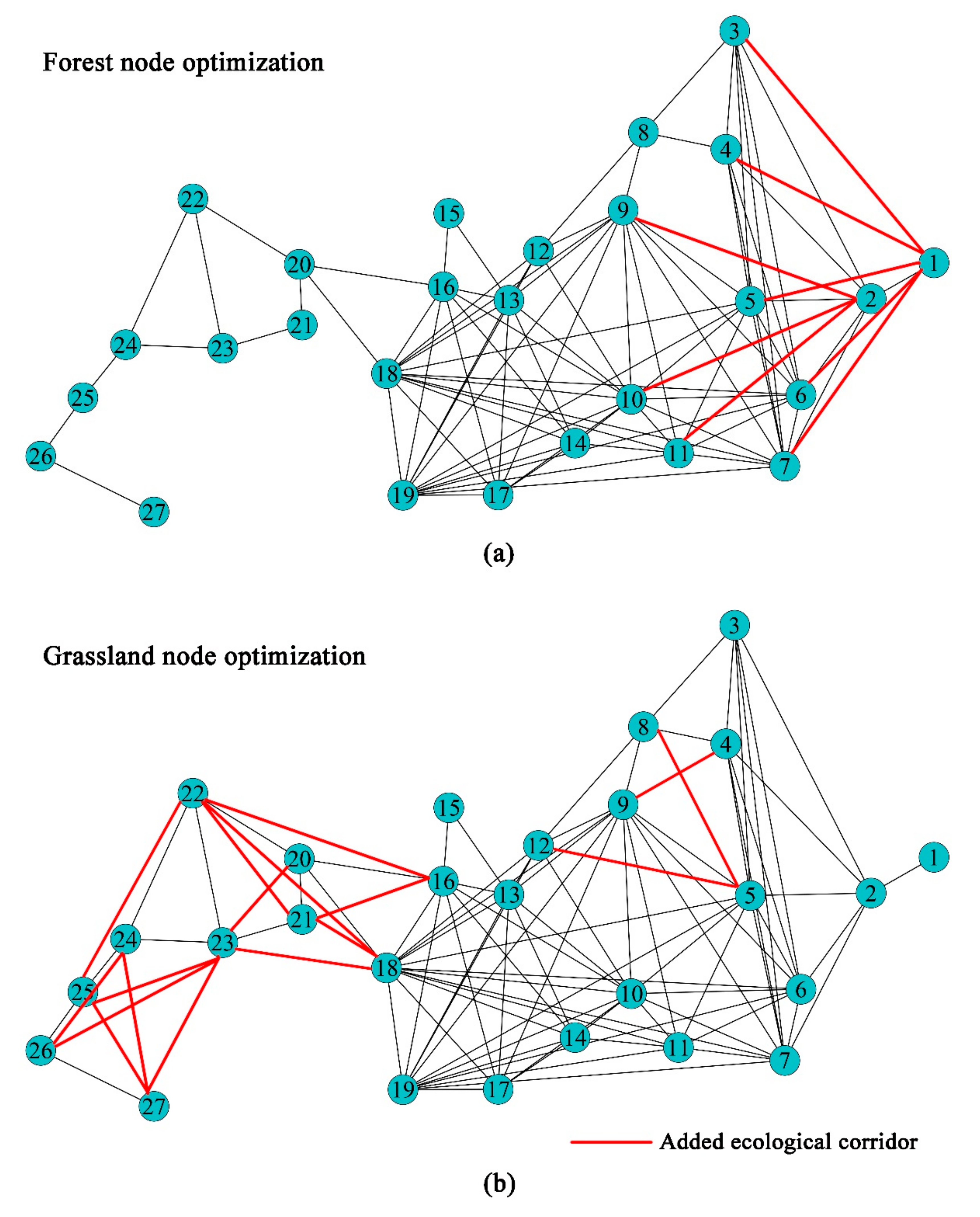
4.2. Suggestions for Optimizing the Vegetation Ecospatial Network in the YRB

Increasing the carbon sequestration capacity of vegetation through the construction of national ecological projects is an important way to achieve carbon neutrality [6]. China is currently in the preparation period of a carbon neutral plan, and several ecological projects may be built in the future. At the same time, the YRB is a key area that requires high-quality development and key conservation [60]. Therefore, network optimization with the aim of increasing the carbon sequestration capacity of vegetation in the YRB is of great interest. In fact, the optimization of the ecospatial network of vegetation in the YRB can be achieved by building national ecological projects. For example, building shelter forests also means increasing ecological corridors between ecological nodes. Returning farmland to forest and grass means increasing vegetation nodes. According to the results in Section 3.4, we provide some ideas for the optimization of the vegetation ecospatial network of the YRB for the purpose of increasing the net carbon sequestration capacity of vegetation. For forest nodes, establishing ecological corridors will increase the shortest path that does not pass through the forest node, thereby reducing the betweenness centrality of the forest node. For grassland nodes, establishing ecological corridors between the neighboring nodes of the grassland node will increase the clustering coefficient of the grassland node.

For the optimization of forest nodes, we selected two forest nodes that were carbon sources in 2018, Node 6 and Node 7, in addition to Node 2, the forest node with the largest betweenness centrality (Table S4). Our optimization strategy was to reduce the betweenness centrality of the nodes by creating ecological corridors and reducing the shortest path through these forest nodes in expectation of increasing the carbon sequestration capacity of the forest nodes. Node 2 served as the only “bridge” between Node 1 and other nodes. Our optimization suggestion is to create ecological corridors between Node 1 and Node 3, Node 4, Node 5, Node 6, and Node 7, thus reducing the betweenness centrality of Node 2. Similarly, Node 6 and Node 7 were the “bridges” between Node 2 and Node 10 and Node 11. The optimization suggestion for Node 6 and Node 7 is to create ecological corridors between Node 2 and Node 10 and Node 11. The optimization results for forest nodes in YRB are shown in Figure 14a.

The ranking of the clustering coefficients of the grassland nodes is shown in Table S5. We find that the clustering coefficients of Node 21, Node 25, Node 26, and Node 27 were all 0, and the clustering coefficients of Node 20 were much lower than those of other nodes, with these five nodes all being carbon source nodes in 2018. In addition, Node 8, Node 9, and Node 24 were carbon source nodes in 2018. These eight carbon source nodes were the optimization targets of the grassland nodes, and the optimization strategy was to establish ecological corridors between the neighboring nodes of these eight grassland nodes to increase the clustering coefficients of these grassland nodes. For example, the neighboring nodes of Node 20 were Node 16, Node 18, Node 21, and Node 22. We built ecological corridors between these neighbor nodes to increase the clustering coefficient of Node 20. In particular, Node 27 had only one neighboring node, Node 26, and we optimized it by adding neighboring nodes. We built ecological corridors between Node 27 and Node 23, Node 24, and Node 25 to increase the neighboring nodes of Node 27. Then, ecological corridors were added between Node 23, Node 24, Node 25, and Node 26 to increase the proportion of connections between neighboring nodes of Node 27, thereby increasing the clustering coefficient of Node 27. Finally, the optimization results for the grassland nodes in the vegetation ecospatial network of the YRB are shown in Figure 14b. Through the establishment of ecological corridors, the optimization of grassland nodes actually increased the connection between Community 2 and Community 1. At the same time, the internal connections of Community 2 were also increased, which facilitates the transmission of information and the exchange of material and energy between the nodes of Community 2.

There have been many studies on the optimization of ecospatial networks, and most of them were based on landscape risk or network stability [20,21,22]. Compared with other studies, the average clustering coefficient of the vegetation ecospatial network constructed in this study is larger and the network structure is relatively more stable. In the background of carbon neutrality, optimization for the purpose of increasing the vegetation carbon sequestration capacity is of more practical significance. However, the above optimization suggestions only provide a reference for decision makers, not the final solution. There are many other options to increase the carbon sequestration capacity of vegetation in reality. For example, some land management measures for forests and grasslands (tending and thinning of forests, enclosure, fertilization, grazing, and returning farmland to grassland) can also increase the carbon sink of forests or grasslands [47,61,62]. In addition, the construction of national ecological projects requires consideration of more practical geographic factors (elevation, slope, slope direction), environmental factors (soil texture, precipitation, temperature), and economic factors (construction cost). The optimization suggestions we made above are only from the perspective of the topology of the network, which is an ideal situation ignoring many practical factors. We will consider more geographic and environmental factors in the future and make a more realistic plan for the national ecological project construction of the YRB by combining the results of this study.

4.3. Prospects and Limitations of This Study

Current studies on ecospatial networks focus more on ecological risks of regions, land desertification, and landscape connectivity and stability [20,63,64,65]. In other words, the current studies on ecospatial networks mainly focus on the spatial pattern. However, the coupling of ecological processes and ecological patterns is an issue that has been explored in landscape ecology [66]. In this study, we found the relationship between the topological characteristics of vegetation and its carbon sequestration capacity, which implies that the spatial pattern described by the ecospatial network is connected with vegetation physiological processes. In addition, a previous study constructed the ecospatial network of Erdos and converted the vegetation carbon sequestration capacity according to the area of vegetation [21]. This has some significance in large-scale studies but may not be fully compatible with reality. The carbon sequestration capacity of vegetation is closely related to the ecophysiological processes of the ecosystem. As shown in the calculation results of the Biome-BGC model in this study, the vegetation ecosystem may be a carbon sink or a carbon source. Therefore, we call on researchers to use mechanism-based ecosystem process models as much as possible when estimating the carbon sequestration capacity of vegetation. Moreover, in addition to the limitations on network optimization mentioned in Section 4.2, this study also has another limitation. The results of this study are only applicable in the YRB, and the choice of study area at different scales may have an impact on the results. In the future, we will conduct similar studies at different scales of the study area to explore the applicability of the findings of this study. In addition, if we face more complex situations (larger amount of data and larger number of topological indicators) in larger-scale study areas, we will consider introducing machine learning methods for data analysis.

5. Conclusions

In this study, we constructed a vegetation ecospatial network in the YRB and calculated multiple topological indicators of the entire network and vegetation nodes. At the same time, we used the Biome-BGC model to calculate the carbon sequestration capacity of vegetation nodes. Then, we analyzed the relationship between the topological indicators and carbon sequestration capacity of vegetation nodes in the YRB, and we made suggestions for the optimization of the network in the background of carbon neutrality. The key conclusions of this study are as follows:

(1)

The vegetation ecospatial network of the YRB in 2018 had a large clustering coefficient, a small-world characteristic, and a relatively stable overall structure. Moreover, the vegetation ecospatial network of the YRB had more carbon sink nodes than carbon source nodes in 2018.

(2)

The net carbon sequestration capacity of forest nodes in the YRB had a negative linear correlation with its betweenness centrality; the carbon sequestration capacity of grassland nodes had a positive linear correlation with its clustering coefficient.

(3)

For the purpose of increasing the carbon sequestration capacity of vegetation, we put forward optimization suggestions for the vegetation ecospatial network in the YRB. In addition, the eastern region of the YRB is a key optimization area for forest nodes, and the western region is a key optimization area for grass nodes.

References

1. IPCC. 2021: Climate Change 2021: The Physical Science Basis. Contribution of Working Group I to the Sixth Assessment Report of the Intergovernmental Panel on Climate Change. Available online: https://www.ipcc.ch/report/ar6/wg1/downloads/report/IPCC_AR6_WGI_Full_Report.pdf. (accessed on 15 October 2021).
2. Broadstock, D.; Ji, Q.; Managi, S.; Zhang, D. Pathways to Carbon Neutrality: Challenges and Opportunities; Elsevier: Amsterdam, The Netherlands, 2021. [Google Scholar]
3. Lu, F.; Hu, H.; Sun, W.; Zhu, J.; Liu, G.; Zhou, W.; Zhang, Q.; Shi, P.; Liu, X.; Wu, X.; et al. Effects of national ecological restoration projects on carbon sequestration in China from 2001 to 2010. Proc. Natl. Acad. Sci. USA 2018, 115, 4039–4044. [Google Scholar] [CrossRef] [Green Version]
4. Fang, J.; Yu, G.; Liu, L.; Hu, S.; Chapin, F.S. Climate change, human impacts, and carbon sequestration in China. Proc. Natl. Acad. Sci. USA 2018, 115, 4015–4020. [Google Scholar] [CrossRef] [Green Version]
5. Wang, Q.; Ni, J.; Tenhunen, J. Application of a geographically-weighted regression analysis to estimate net primary production of Chinese forest ecosystems. Glob. Ecol. Biogeogr. 2005, 14, 379–393. [Google Scholar] [CrossRef]
6. Ding, Z.L. Research on China’s Carbon Neutrality Framework Roadmap. China Ind. Inf. Technol. 2021, 8, 54–61. [Google Scholar]
7. Diodato, N.; Bellocchi, G. Spatial probability modelling of forest productivity indicator in Italy. Ecol. Indic. 2019, 108, 105721. [Google Scholar] [CrossRef]
8. Jiang, H.; Apps, M.J.; Zhang, Y.; Peng, C.; Woodard, P.M. Modelling the spatial pattern of net primary productivity in Chinese forests. Ecol. Model. 1999, 122, 275–288. [Google Scholar] [CrossRef]
9. Chen, J.M.; Ju, W.; Cihlar, J.; Price, D.; Liu, J.; Chen, W.; Pan, J.; Black, A.; Barr, A. Spatial distribution of carbon sources and sinks in Canada’s forests. Tellus Chem. Phys. Meteorol. 2003, 55, 622–641. [Google Scholar] [CrossRef] [Green Version]
10. Gu, F.; Zhang, Y.; Huang, M.; Tao, B.; Guo, R.; Yan, C. Effects of climate warming on net primary productivity in China during 1961–2010. Ecol. Evol. 2017, 7, 6736–6746. [Google Scholar] [CrossRef]
11. Duveneck, M.J.; Thompson, J.R. Climate change imposes phenological trade-offs on forest net primary productivity. J. Geophys. Res. Biogeosci. 2017, 122, 2298–2313. [Google Scholar] [CrossRef]
12. Tobler, W.R. A Computer Movie Simulating Urban Growth in the Detroit Region. Econ. Geogr. 1970, 46, 234–240. [Google Scholar] [CrossRef]
13. Chang, D.H.S.; Gauch, H.G., Jr. Multivariate analysis of plant communities and environmental factors in Ngari, Tibet. Ecology 1986, 67, 1568–1575. [Google Scholar] [CrossRef]
14. Wu, Z.; Lin, C.; Su, Z.; Zhou, S.; Zhou, H. Multiple landscape “source–sink” structures for the monitoring and management of non-point source organic carbon loss in a peri-urban watershed. Catena 2016, 145, 15–29. [Google Scholar] [CrossRef]
15. Wu, Y.; Wang, D.; Qiao, X.; Jiang, M.; Li, Q.; Gu, Z.; Liu, F. Forest dynamics and carbon storage under climate change in a subtropical mountainous region in central China. Ecosphere 2020, 11, e03072. [Google Scholar] [CrossRef]
16. Liu, X.; Li, X.; Chen, Y.; Tan, Z.; Li, S.; Ai, B. A new landscape index for quantifying urban expansion using multi-temporal remotely sensed data. Landsc. Ecol. 2010, 25, 671–682. [Google Scholar] [CrossRef]
17. Costa, L.D.F.; Rodrigues, F.A.; Travieso, G.; Boas, P.R.V. Characterization of complex networks: A survey of measurements. Adv. Phys. 2007, 56, 167–242. [Google Scholar] [CrossRef] [Green Version]
18. Bombrun, M.; Dash, J.P.; Pont, D.; Watt, M.S.; Pearse, G.D.; Dungey, H. Forest-Scale Phenotyping: Productivity Characterisation Through Machine Learning. Front. Plant Sci. 2020, 11, 99. [Google Scholar] [CrossRef] [PubMed]
19. Albert, R.; Barabási, A.-L. Statistical mechanics of complex networks. Rev. Mod. Phys. 2002, 74, 47–97. [Google Scholar] [CrossRef] [Green Version]
20. Yu, Q.; Yue, D.; Wang, Y.; Kai, S.; Fang, M.; Ma, H.; Zhang, Q.; Huang, Y. Optimization of ecological node layout and stability analysis of ecological network in desert oasis: A typical case study of ecological fragile zone located at Deng Kou County (Inner Mongolia). Ecol. Indic. 2018, 84, 304–318. [Google Scholar] [CrossRef]
21. Guo, H.; Yu, Q.; Pei, Y.; Wang, G.; Yue, D. Optimization of landscape spatial structure aiming at achieving carbon neutrality in desert and mining areas. J. Clean. Prod. 2021, 322, 129156. [Google Scholar] [CrossRef]
22. Xu, W.; Wang, J.; Zhang, M.; Li, S. Construction of landscape ecological network based on landscape ecological risk assessment in a large-scale opencast coal mine area. J. Clean. Prod. 2021, 286, 125523. [Google Scholar] [CrossRef]
23. Watt, M.S.; Palmer, D.J.; Dungey, H.; Kimberley, M.O. Predicting the spatial distribution of Cupressus lusitanica productivity in New Zealand. For. Ecol. Manag. 2009, 258, 217–223. [Google Scholar] [CrossRef]
24. Su, H.Z. Analyzing and Simulating the Growth of Picea Schrenkiana Forests in Xinjiang under Global Climate Change. Ph.D Thesis, Institute of Botany, the Chinese Academy of Sciences, Beijing, China, 2005. [Google Scholar]
25. Chen, Y.-P.; Fu, B.-J.; Zhao, Y.; Wang, K.-B.; Zhao, M.M.; Ma, J.-F.; Wu, J.-H.; Xu, C.; Liu, W.-G.; Wang, H. Sustainable development in the Yellow River Basin: Issues and strategies. J. Clean. Prod. 2020, 263, 121223. [Google Scholar] [CrossRef]
26. Wang, F.; Wang, Z.; Yang, H.; Zhao, Y.; Li, Z.; Wu, J. Capability of Remotely Sensed Drought Indices for Representing the Spatio–Temporal Variations of the Meteorological Droughts in the Yellow River Basin. Remote Sens. 2018, 10, 1834. [Google Scholar] [CrossRef] [Green Version]
27. Wohlfart, C.; Liu, G.; Huang, C.; Kuenzer, C. A River Basin over the Course of Time: Multi-Temporal Analyses of Land Surface Dynamics in the Yellow River Basin (China) Based on Medium Resolution Remote Sensing Data. Remote Sens. 2016, 8, 186. [Google Scholar] [CrossRef] [Green Version]
28. Sheng, W.; Zhen, L.; Xiao, Y.; Hu, Y. Ecological and socioeconomic effects of ecological restoration in China’s Three Rivers Source Region. Sci. Total Environ. 2019, 650, 2307–2313. [Google Scholar] [CrossRef] [PubMed]
29. Zhao, G.; Tian, P.; Mu, X.; Jiao, J.; Wang, F.; Gao, P. Quantifying the impact of climate variability and human activities on streamflow in the middle reaches of the Yellow River basin, China. J. Hydrol. 2014, 519, 387–398. [Google Scholar] [CrossRef]
30. Guan, B.; Chen, M.; Quirk, T.; Yang, S.; Shang, W.; Li, Y.; Tian, X.; Han, G. Soil seed bank and vegetation differences following channel diversion in the Yellow River Delta. Sci. Total Environ. 2019, 693, 133600. [Google Scholar] [CrossRef] [PubMed]
31. Wang, S.; Fu, B.; Piao, S.; Lü, Y.; Ciais, P.; Feng, X.; Wang, Y. Reduced sediment transport in the Yellow River due to anthropogenic changes. Nat. Geosci. 2016, 9, 38–41. [Google Scholar] [CrossRef]
32. Zhang, W.; Wang, L.; Xiang, F.; Qin, W.; Jiang, W. Vegetation dynamics and the relations with climate change at multiple time scales in the Yangtze River and Yellow River Basin, China. Ecol. Indic. 2020, 110, 105892. [Google Scholar] [CrossRef]
33. Wu, B.; Zeng, Y.; Zhao, D. Land cover mapping and above ground biomass estimation in China. In Proceedings of the 2016 IEEE International Geoscience and Remote Sensing Symposium (IGARSS), Beijing, China, 10–15 July 2016; pp. 3535–3536. [Google Scholar]
34. Chen, L.; Fu, B.; Zhao, W. Source-sink landscape theory and its ecological significance. Front. Biol. China 2008, 3, 131–136. [Google Scholar] [CrossRef]
35. Running, S.; Zhao, M. MOD17A3HGF MODIS/Terra Net Primary Production Gap-Filled Yearly L4 Global 500m SIN Grid V006. Available online: https://doi.org/10.5067/MODIS/MOD17A3HGF (accessed on 24 November 2021).
36. Xu, H. A study on information extraction of water body with the modified normalized difference water index (MNDWI). J. Remote Sens. 2005, 5, 589–595. [Google Scholar]
37. Wu, J.; Zhang, Y.; Zhang, J.; Fan, S.; Yang, C.; Zhang, X. Comparison and analysis of water indexes in muddy coasts based on MODIS data: A case study of the Yellow River Delta coast. Remote Sens. Land Resour. 2019, 3, 242–249. [Google Scholar]
38. Shi, F.; Liu, S.; Sun, Y.; An, Y.; Zhao, S.; Liu, Y.; Li, M. Ecological network construction of the heterogeneous agro-pastoral areas in the upper Yellow River basin. Agric. Ecosyst. Environ. 2020, 302, 107069. [Google Scholar] [CrossRef]
39. Yu, Q.; Yue, D.; Wang, J.; Zhang, Q.; Li, Y.; Yu, Y.; Chen, J.; Li, N. The optimization of urban ecological infrastructure network based on the changes of county landscape patterns: A typical case study of ecological fragile zone located at Deng Kou (Inner Mongolia). J. Clean. Prod. 2017, 163, S54–S67. [Google Scholar] [CrossRef]
40. Su, K.; Yu, Q.; Yue, D.; Zhang, Q.; Yang, L.; Liu, Z.; Niu, T.; Sun, X. Simulation of a forest-grass ecological network in a typical desert oasis based on multiple scenes. Ecol. Model. 2019, 413, 108834. [Google Scholar] [CrossRef]
41. Knaapen, J.P.; Scheffer, M.; Harms, B. Estimating habitat isolation in landscape planning. Landsc. Urban. Plan. 1992, 23, 1–16. [Google Scholar] [CrossRef]
42. Jiang, W.; Yuan, L.; Wang, W.; Cao, R.; Zhang, Y.; Shen, W. Spatio-temporal analysis of vegetation variation in the Yellow River Basin. Ecol. Indic. 2015, 51, 117–126. [Google Scholar] [CrossRef]
43. Koschützki, D.; Lehmann, K.A.; Peeters, L.; Richter, S.; Tenfelde-Podehl, D.; Zlotowski, O. Centrality Indices. In Network Analysis; Brandes, U., Erlebach, T., Eds.; Springer: Berlin/Heidelberg, Germany, 2005; pp. 16–61. [Google Scholar]
44. Jing, Y.; Baluja, S. Pagerank for product image search. In Proceeding of the 17th International Conference on World Wide Web, Beijing, China, 21–25 April 2008; pp. 307–316. [Google Scholar]
45. Newman, M.E.J. Modularity and community structure in networks. Proc. Natl. Acad. Sci. USA 2006, 103, 8577–8582. [Google Scholar] [CrossRef] [PubMed] [Green Version]
46. Fang, J.Y.; Ke, J.H.; Tang, Z.Y.; Chen, A.P. Implications and estimations of four terrestrial productivity parameters. Chin. J. Plant Ecol. 2001, 25, 414. [Google Scholar]
47. Allard, V.; Soussana, J.-F.; Falcimagne, R.; Berbigier, P.; Bonnefond, J.; Ceschia, E.; D’Hour, P.; Hénault, C.; Laville, P.; Martin, C.; et al. The role of grazing management for the net biome productivity and greenhouse gas budget (CO2, N2O and CH4) of semi-natural grassland. Agric. Ecosyst. Environ. 2007, 121, 47–58. [Google Scholar] [CrossRef]
48. Thornton, P.; Law, B.; Gholz, H.L.; Clark, K.L.; Falge, E.; Ellsworth, D.; Goldstein, A.; Monson, R.; Hollinger, D.; Falk, M.; et al. Modeling and measuring the effects of disturbance history and climate on carbon and water budgets in evergreen needleleaf forests. Agric. For. Meteorol. 2002, 113, 185–222. [Google Scholar] [CrossRef]
49. Ichii, K.; Hashimoto, H.; Nemani, R.; White, M. Modeling the interannual variability and trends in gross and net primary productivity of tropical forests from 1982 to 1999. Glob. Planet. Chang. 2005, 48, 274–286. [Google Scholar] [CrossRef]
50. Jia, X.; Shao, M.; Yu, D.; Zhang, Y.; Binley, A. Spatial variations in soil-water carrying capacity of three typical revegetation species on the Loess Plateau, China. Agric. Ecosyst. Environ. 2019, 273, 25–35. [Google Scholar] [CrossRef] [Green Version]
51. Sánchez-Ruiz, S.; Maselli, F.; Chiesi, M.; Fibbi, L.; Martinez, B.; Campos-Taberner, M.; García-Haro, F.J.; Gilabert, M.A. Remote Sensing and Bio-Geochemical Modeling of Forest Carbon Storage in Spain. Remote Sens. 2020, 12, 1356. [Google Scholar] [CrossRef]
52. Turner, D.P.; Ritts, W.D.; Cohen, W.B.; Gower, S.T.; Running, S.W.; Zhao, M.; Costa, M.; Kirschbaum, A.A.; Ham, J.M.; Saleska, S.R.; et al. Evaluation of MODIS NPP and GPP products across multiple biomes. Remote Sens. Environ. 2006, 102, 282–292. [Google Scholar] [CrossRef]
53. Hasenauer, H.; Petritsch, R.; Zhao, M.; Boisvenue, C.; Running, S.W. Reconciling satellite with ground data to estimate forest productivity at national scales. For. Ecol. Manag. 2012, 276, 196–208. [Google Scholar] [CrossRef]
54. Li, X.-H.; Sun, O.J. Testing parameter sensitivities and uncertainty analysis of Biome-BGC model in simulating carbon and water fluxes in broadleaved-Korean pine forests. Chin. J. Plant Ecol. 2018, 42, 1131–1144. [Google Scholar] [CrossRef]
55. Zhang, Q.B. Study on the Construction and Optimization of Ecological Network in the Northeastern Margin of Ulanbuhe Desert. Ph.D. Thesis, Beijing Forestry University, Beijing, China, 2019. [Google Scholar]
56. Watts, D.J.; Strogatz, S.H. Collective dynamics of ‘small-world’ networks. Nature 1998, 393, 440–442. [Google Scholar] [CrossRef]
57. Bodin, Ö.; Alexander, S.M.; Baggio, J.; Barnes, M.; Berardo, R.; Cumming, G.S.; Dee, L.E.; Fischer, A.P.; Fischer, M.; Garcia, M.M.; et al. Improving network approaches to the study of complex social–ecological interdependencies. Nat. Sustain. 2019, 2, 551–559. [Google Scholar] [CrossRef]
58. Xie, J.; Szymanski, B.K. Community detection using a neighborhood strength driven Label Propagation Algorithm. In Proceedings of the 2011 IEEE Network Science Workshop, New York, NY, USA, 22–24 June 2011. [Google Scholar]
59. Goodchild, M.F. The Validity and Usefulness of Laws in Geographic Information Science and Geography. Ann. Assoc. Am. Geogr. 2004, 94, 300–303. [Google Scholar] [CrossRef] [Green Version]
60. Xi, J.P. Speech at the Symposium on Ecological Protection and Quality Development of the Yellow River Basin. China Water Resour. 2019, 20, 1–3. [Google Scholar]
61. Boisvenue, C.; Running, S. Simulations show decreasing carbon stocks and potential for carbon emissions for Rocky Mountain forests in the next century. Ecol. Appl. 2009, 20, 1302–1319. [Google Scholar] [CrossRef] [PubMed]
62. Bustamante, M.; Robledo-Abad, C.; Harper, R.; Mbow, C.; Ravindranat, N.H.; Sperling, F.; Haberl, H.; Pinto, A.D.S.; Smith, P. Co-benefits, trade-offs, barriers and policies for greenhouse gas mitigation in the agriculture, forestry and other land use (AFOLU) sector. Glob. Chang. Biol. 2014, 20, 3270–3290. [Google Scholar] [CrossRef] [PubMed] [Green Version]
63. Cui, L.; Wang, J.; Sun, L.; Lv, C. Construction and optimization of green space ecological networks in urban fringe areas: A case study with the urban fringe area of Tongzhou district in Beijing. J. Clean. Prod. 2020, 276, 124266. [Google Scholar] [CrossRef]
64. Nie, W.; Shi, Y.; Siaw, M.J.; Yang, F.; Wu, R.; Wu, X.; Zheng, X.; Bao, Z. Constructing and optimizing ecological network at county and town Scale: The case of Anji County, China. Ecol. Indic. 2021, 132, 108294. [Google Scholar] [CrossRef]
65. Huang, X.; Wang, H.; Shan, L.; Xiao, F. Constructing and optimizing urban ecological network in the context of rapid urbanization for improving landscape connectivity. Ecol. Indic. 2021, 132, 108319. [Google Scholar] [CrossRef]
66. Fu, B.; Liang, D.; Lu, N. Landscape ecology: Coupling of pattern, process, and scale. Chin. Geogr. Sci. 2011, 21, 385–391. [Google Scholar] [CrossRef]
Figure 1. Schematic diagram of the geographical location of the Yellow River Basin. A, B, and C are the areas facing ecological problems in the upstream, middle and upper reaches, and downstream, respectively. The right panel indicates the location of this study area in China.
Remotesensing 13 04926 g001
Figure 2. Flowchart of MODIS product processing.
Remotesensing 13 04926 g002
Figure 3. Schematic diagram of the study framework.
Remotesensing 13 04926 g003
Figure 4. Results of factors for constructing ecospatial networks. The unit of NPP is g·C m−2·year−1. The unit of DEM is m. The unit of slope is °. The other factors are dimensionless.
Remotesensing 13 04926 g004
Figure 5. Map of the ecological sources of the Yellow River Basin.
Remotesensing 13 04926 g005
Figure 6. Cumulative resistance surface distribution map.
Remotesensing 13 04926 g006
Figure 7. The result map of the ecospatial network of the Yellow River Basin.
Remotesensing 13 04926 g007
Figure 8. The distribution graph of the degree of ecological nodes, representing a topology simplification of the ecospatial network. The size of the node in the graph represents its degree. The number on the node represents its serial number.
Remotesensing 13 04926 g008
Figure 9. The results of five topological indicators of ecological nodes.
Remotesensing 13 04926 g009
Figure 10. The result of community division of ecological nodes. The node size represents the clustering coefficient.
Remotesensing 13 04926 g010
Figure 11. The spatial distribution map of the NBP results of the ecological nodes in the Yellow River Basin in 2018.
Remotesensing 13 04926 g011
Figure 12. Comparison of NBP and NPP trends for all vegetation nodes; r indicates the Pearson’s correlation coefficient.
Remotesensing 13 04926 g012
Figure 13. (a) Pearson’s correlation coefficients matrix between the topological indicators of the ecological nodes and the NBP. Blue indicates positive correlation; red indicates negative correlation. A darker color indicates greater correlation. The asterisks denote statistical significance: * p < 0.05, ** p < 0.01. (b) The result of linear regression analysis of betweenness centrality of forest nodes and NBP. (c) The result of linear regression analysis of clustering coefficient of grassland nodes and NBP.
Remotesensing 13 04926 g013
Figure 14. (a) Schematic diagram of optimization suggestions for forest nodes in the Yellow River Basin. (b) Schematic diagram of optimization suggestions for grassland nodes in the Yellow River Basin.
Remotesensing 13 04926 g014