The Performance of the Diurnal Cycle of Precipitation from Blended Satellite Techniques over Brazil

Abstract

The knowledge of the diurnal cycle of precipitation is of extreme relevance to understanding the physical/dynamic processes associated with the spatial and temporal distribution of precipitation. The main difficulty of this task is the lack of surface precipitation information over certain regions on an hourly time scale and the low spatial representativeness of these data (normally surface gauges). In order to overcome these difficulties, the main objective of this study is to create a 3-h precipitation accumulation database from the gauge-adjusted daily regional precipitation products to resolve the diurnal cycle properly. This study also proposes to evaluate different methodologies for partitioning gauge-adjusted daily precipitation products, i.e., a product made by the combination of satellite estimates and surface gauge observations, into 3-h precipitation accumulation. Two methodologies based on the calculation of a conversion factor F between a daily gauge-adjusted product, combined scheme (CoSch, hereafter), and a non-gauge-adjusted one, the integrated multi-satellite retrievals for GPM (IMERG)-Early (IMERG, hereafter) were tested for this research. Hourly rain gauge stations for the period of 2015–2018 over Brazil were used to assess the performance of the proposed methodologies over the whole region and five sub-regions with homogeneous precipitation regimes. Standard statistical metrics and categorical indices related with the capability to detect rainfall events were used to compare the ability of each product to represent the diurnal cycle. The results show that the new 3-h CoSch products show better agreement with rainfall gauge stations when compared with IMERG, better capturing the diurnal cycle of precipitation. The biggest improvement was over northeastern region close to the coast, where IMERG was not able to capture the diurnal cycle properly. One of the proposed methodologies (CoSchB) performed better on the critical success index and equitable threat score metrics, suggesting that this is the best product over the two. The downside, when compared with the other methodology (CoSchA), was a slight increase in the values of bias and mean absolute error, but still at acceptable levels.

1. Introduction

The knowledge of the freshwater distribution across the globe is of vital importance for the management of natural resources, and precipitation is a central component of the hydrological cycle, transferring water inside the earth–atmosphere system. The intrinsic high temporal and spatial variability of precipitation patterns over a given region are an obstacle to understanding those characteristics. A way to address those issues is to systematically examine the timing and duration of precipitation events as a function of time of day [1], since precipitation is modulated by the variability of solar activity (diurnal cycle). The solar radiation diurnal cycle changes the surface temperature, causing variations in the convection and cloud formation patterns and, consequently, the precipitation itself. Therefore, the study of the precipitation diurnal cycle (PDC, hereafter) is important not only in understanding the physical processes involved in precipitation generation, but also to evaluate the performance of weather, climate and hydrology models [2,3,4,5], being a key factor in understanding rainfall variability. In general, convection processes generate a maximum of rainfall in the afternoon and a minimum in the morning on continental surfaces, while the opposite occurs over the ocean, resulting from the sea/land breeze mesoscale circulation [6]. While these are the most significant dynamically forced diurnal rainfall regimes across the globe, studies suggest a larger variety of PDC regimes over Brazil. For example, Brito et al. [7] studied in details the different PDC regimes over the continent and adjacent oceanic areas in northern Brazil, suggesting a new type of regime with a maximum precipitation in the morning (seaside coastal influence) and another in late afternoon (continental influence). More recently, a study of Afonso et al. [8] identified seven regions with different PDC characteristics over Brazil and shows that satellite precipitation algorithms are better in those regions where thermal-induced heating produces deep convective clouds than those regions driven by shallow convection or low-level circulation.

The rain gauge networks and weather radars are the main source of precipitation information overground, but they have limited coverage and, in the case of rain gauges, limited representativeness. These issues lead to uncertainties for the study of precipitation processes. In this context, satellite-based estimates become a complementary tool for monitoring precipitation. Geostationary satellite sensors have been used to estimate precipitation since the 1980s at cloud scales with low latency and high spatial resolution, but with limitations due to uncertainties on the relationships between cloud top brightness temperature and surface precipitation on the infrared and visible spectrum. To overcome these limitations, low-orbit microwave satellite sensors started to be used with the advantage to provide more accurate estimates, because of the ability of microwave radiation to penetrate clouds, being sensitive to liquid (water) and solid (ice) hydrometeors. The downside of passive microwave (PMW) retrievals are the higher latency and lower spatial and temporal resolution data, because of the low-orbit scan and the portion of electromagnetic spectrum used to retrieve rainfall.

Although improvements have been made on satellite precipitation estimation techniques over the years, there are still systematic errors due to regional and seasonal rainfall regimes, and possible random errors, due to the indirect nature of these measurements [9]. In order to minimize these errors, several blended techniques combining satellite data with rain gauge data have been or are being developed. Linear regression models [10], the calculation of residuals weighted by the inverse of distance [11], coupling with numerical models [12,13,14], and geostatistical techniques such as kriging [15] and others [16] are among the most utilized methodologies to perform these blending techniques.

Considering the lack of surface precipitation information on the time scale of hours over certain regions in Brazil [8] and South America [17], and the low spatial representativeness of these data, the main objective of this study is to create a 3-h precipitation accumulation database from the gauge-adjusted (hereafter called blended) daily regional precipitation products (i.e., a product made by the combination of satellite estimates and surface gauge observations) in order to resolve the diurnal cycle properly. While there are several algorithms with temporal resolution of 30 min, such as the integrated multi-satellite retrievals for GPM (IMERG) [18] and the climate prediction center morphing method (CMORPH) [19], they are not normally gauge-corrected at a daily basis and, when they are, the latency could be of several days. The use of regional daily blended products [20] also means that regional gauge networks could be accessed and more rain gauge stations are included in the blended product. Finally, different methodologies for the creation of the new database can be evaluated in order to provide the better product for the user’s community.

This article is structured as follows: Section 2 presents information from the study areas, precipitation data sets, and statistics metrics used in the validation process. Section 3 presents the main results of this research and discussion, while the conclusions are provided in Section 4.

2. Materials and Methods

2.1. Study Area

Brazil occupies most of the central and eastern part of the South America continent, with its coast bordering a large part of the Atlantic Ocean. With an area of approximately 8,514,215 km², it presents a great diversity of landscapes, biodiversity, climate, and precipitation regimes [8]. While this study is focused on Brazil at a larger scale, because of its continental dimensions, it is important to consider the influence of different precipitation regimes. To account for that, the present study opted to continue the work of Rozante et al. [21], who evaluated daily blended products over five regions with a different rainfall regime (R1 to R5 see Figure 1). Those regions were created based on analysis over an 18-year time span precipitation database. The region R1 presents well-distributed precipitation year-round and is largely influenced by transient frontal systems that carry cold air masses from temperate and subtropical regions. The R2 covers a large area of Brazil encompassing the west part of the north region and all the center-west and southeast regions. With high influence from the South Atlantic convergence zone (SACZ), this region is characterized by higher precipitation levels in summer (December, January and February (DJF)) than winter (June, July and August (JJA)). The R3 region, located on the northeast of Brazil, has the lowest accumulated values of precipitation, because of large-scale subsidence patterns inhibiting cloud formation, and does not present a well-defined rainfall regime. The R4 is located on the coast of Brazil’s northeast region and presents higher precipitation during JJA than DJF, and is influenced by the sea breeze circulation. Finally, the R5 region has the highest accumulated values of precipitation over Brazil, due to the Intertropical convergence zone (ITCZ), covering the northern part of the north region. The period of maximum precipitation occurs during January, February and March (JFM).

In this study, six regions were considered, including the Brazil (BR) study area region that covers the whole country. Therefore, we have the BR box and the R1–R5 sub-regions, all of which are shown in Figure 1. More details including the data processing and validation process are in the subsequent sections.

2.2. IMERG Precipitation Estimates Data

The IMERG algorithm [18] is responsible for intercalibrating, merging, and interpolating all satellite microwave precipitation estimates, together with microwave-calibrated infrared satellite estimates (IMERG-Early and IMERG-Late products) and precipitation gauge observations for bias correction purposes (IMERG-Final), but employing the GPM constellation of satellites. The GPM is considered the successor of Tropical Rainfall Measuring Mission (TRMM) multi-satellite precipitation analysis (TMPA) [22] and has significant improvements. The orbital inclination has been increased from 35° to 65°, resulting in greater global coverage, the radar has been upgraded to two frequencies, adding sensitivity to light precipitation, and the channels of 165.5 and 183.3 GHz were added to the passive microwave sensor imager, which facilitates the detection of light and solid precipitation [23]. The observation interval for GPM is also 30 min instead of the 3 h interval for TRMM. The IMERG data are produced by a Bayesian inverse algorithm applied to microwave brightness temperatures that is run several times for each observation time [24]. The spatial resolution is 0.1° with 30 min of temporal resolution. However, to match the resolution of gauges data, the data were converted to tri-hourly temporal resolution. The IMERG-Early version (hereafter, IMERG) for the period of 2015–2018 were used for the creation of the new 3-h blended and daily products (see Section 2.3) and also for as a benchmark for low-latency sub-daily products.

2.3. Combined Scheme (CoSch) Precipitation Data

Combined scheme (CoSch) is a regional daily blended precipitation product obtained with the combination of satellite precipitation estimates and daily gauge observations data [25]. The methodology is based on the bias correction between satellite and gauge data, where additive and multiplicative bias correction schemes are applied for each gauge station on a daily basis. Initially, the rain gauge observations are interpolated with the nearest neighbor method to match the grid size of the satellite estimates where all regions with a distance greater than five grid points from the closest station are masked out. In the remaining regions, the difference between additive/multiplicative bias correction and observed values is performed. The mean additive and multiplicative bias corrections schemes are calculated, respectively, by:

$$CA=sat+cadd=sat+\overline{\left(ob{s}^i-sa{t}^i\right)}$$

(1)

$$CM=sat\ast cmult=sat\ast \overline{\left(ob{s}^i/sa{t}^i\right)},$$

(2)

where i represents a gauge station, sat is the precipitation value estimated by satellite and obs is the value observed by a gauge station. The values of cadd and cmult are, respectively, the additive and multiplicative bias for each station i and the bar represents the process of gridding the data. One particular scheme (additive or multiplicative) is selected for each grid point based on the minimum difference (CA or CM) between that particular bias correction and the observation. The bias-corrected precipitation in the rest of the land areas masked out is defined as a weight average of the additive and multiplicative bias correction schemes as follows:

$$CoSc{h}_i=\alpha C{A}_i+\beta C{M}_i$$

(3)

where i represents a grid point and CoSch_i is the final result for the CoSch scheme. The weight factors α and β represent the number of times a particular scheme is selected in a 3° × 3° box centered in the grid box with i divided by the total grid points in that particular box (excluded all masked points) so that α + β = 1 for every non-masked grid point.

For this study, the CoSch scheme was applied to daily IMERG precipitation estimates for the period of 2015–2018 and applied to the creation of the blended 3-h products. Although similar daily blended products are available on a global scale, like IMERG-Final, CoSch was chosen because it performs better over South America [20].

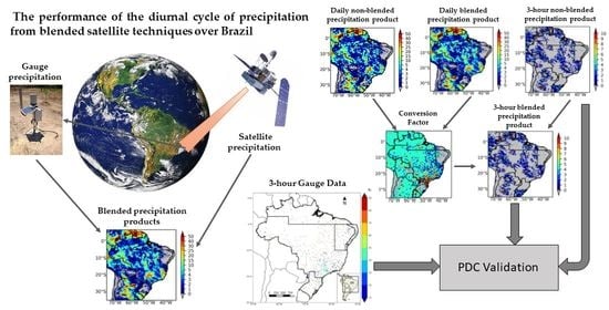
2.4. Methodologies for 3-h Database Development

The main philosophy behind the partition of daily data was to transfer the gauge calibration information on the blended precipitation product in some way to the 3-h version. To accomplish this, a conversion factor F was calculated between the blended and the non-blended versions as follows:

$$F=\{\begin{array}{c}{P}_{B-D}/P_{NB-D},\mathrm{when}{P}_{NB-D}\ne 0\iff P_{B-D}=Fx{P}_{NB-D}\\ 0,\mathrm{when}{P}_{NB-D}=0\\ 0,\mathrm{when}{P}_{B-D}=0\mathrm{and}{P}_{NB-D}=0\end{array}$$

(4)

where P_B-D and P_NB-D are, respectively, the blended and the non-blended daily precipitation products. In this case, the blended product is CoSch (see Section 2.3) and the non-blended product is IMERG. The F values in the previous step were calculated on a daily basis and were applied to the creation of the 3-h product version so that:

$$P_{B,i}=Fx{P}_{NB,i}$$

(5)

where P_B,i and P_NB,i are, respectively, the 3-h versions of P_B-D (the new adjusted product) and P_NB-D (the existent non-gauge-adjusted product). The subscript i represents time ranging from 1 to 8 (00Z, 03Z…,21Z) and, by construction, the sum of the eight partitions is the 24 h accumulated daily precipitation, except for those pixels where P_B-D is different to zero and P_NB-D is zero on that particular day. In such a case, with F = 0, the sum of the eight periods is zero and P_B is not zero. In order to overcome this issue, in those grid points where this particular situation occurs, P_B,i is calculated by the following equation:

$$P_{B,i}=P{F}_{clim,i}x{P}_{B-D}={\left(P_{NB,i}/P_{NB-D}\right)}_{clim,i}x{P}_{B-D}$$

(6)

where PF_clim,i is the four-month period climatology (Jan–Apr, May–Aug and Sep–Dec) of the daily precipitation fraction on time i, and represents the fraction amount of the daily precipitation that is expected to occur at time i. Figure 2 shows the maps of PF_clim,i calculated for the BR region.

Figure 3 shows a flow diagram to create the 3-h version product with IMERG and CoSch datasets. From the daily products of IMERG and CoSch, the conversion factor F is calculated and applied to the 3-h IMERG product resulting in the blended 3-h CoSch product. In those grid points where CoSch is not zero and IMERG is zero, the CoSch daily values are multiplied by the PF_clim,i values.

In order to evaluate if the climatological factor (PF_clim,i) has a positive impact on the new product, two CoSch blended 3-h products were created and they were named CoSchA, where those grid points with climatological correction were excluded, and CoSchB, where those points were included in the statistics. Because the number of points where PF_clim,i was used is relatively small compared with those points where F is performed, a large difference is not expected between both products. However, the number of points is enough to test the sensitivity of the proposed method as shown in the results section (see Section 3). Figure 4 shows an example of the CoSchB methodology for 01/01/2018 at 03Z.

2.5. Gauges Validation Process

2.5.1. Gauge Data

The hourly precipitation gauge data was provided by the National Institute for Space Research (INPE) for the period of 2015–2018 in the form of a compilation from several agencies [8], including the Brazilian National Institute of Meteorology (INMET), the National Water Agency (ANA), Companhia Energética de Minas Gerais (CEMIG), Agronomic Institute (IAC) and Sistema Meteorológico do Paraná (SIMEPAR). A quality control was performed to exclude unrealistic values, check convective rainfall ratios with satellite imagery and account for differences in the time resolution data between the agencies. At the end of the quality control, a total of 1261 stations were selected. The data were interpolated to a 0.1 × 0.1 grid using the simple average for the rain gauges station available at each grid point (Figure 5) and has a temporal resolution of 3 h. It is possible to see that the sampling frequency of data is quite uneven along Brazil, with relatively low values (less than 40% of the total series) for some points in southeastern and southern Brazil. More information about the gauge data processing, quality control and the cluster analysis performed to obtain the chosen sub regions are in Afonso et al. [8].

2.5.2. Performance and Statistic Metrics

The main purpose of this validation study is to provide accurate information regarding the regional and seasonal performance of the two CoSch blended 3-h products. Both were quantitatively and systematically assessed by using some standard statistical metrics and categorical indices including: the bias (error between satellite precipitation estimates and observed precipitations); the mean absolute error (MAE); the root mean square error (RMSE); the Pearson linear correlation coefficient (r) between satellite precipitation estimates and observed precipitations; the bias score (BSCORE), which is the relationship between frequencies of estimated event versus frequency of observed event; the probability of detection (POD), which is the fraction of corrected estimated events; the false alarm ratio (FAR), which is the fraction of estimated events that did not occur; and the equitable threat score (ETS), which measures the fraction of estimated and/or observed events that were correctly predicted, but adjusted by a factor (H_r) based on hits associated with random chance. r is a dimensionless variable whereas bias, MAE, and RMSE are in units of mm/3 h. BSCORE, POD, FAR and ETS are categorical indices related to the capability of detection of rainfall events. More details about the definition of these indices can be found in Wilks [26], while

Table 1. List of the statistical indices mentioned in this study. The size of sample is represented by n, while P and O are, respectively, the estimated (satellite) and observed (gauges) precipitation values.

Statistic Index	Equation	Unit	Best Value
Pearson’s Linear Correlation Coefficient	$r=\frac{{{\displaystyle \sum }}_{i=1}^n\left(P_i-\overline{P}\right){{\displaystyle \sum }}_{i=1}^n\left(O_i-\overline{O}\right)}{\sqrt{{\left(P_i-\overline{P}\right)}^2}\sqrt{{\left(O_i-\overline{O}\right)}^2}}$	-	1
Bias	$bias=\frac{{{\displaystyle \sum }}_{i=1}^n\left(P_i-O_i\right)}{n}$	mm/3 h	0
Mean Absolute Error	$MAE=\frac{{{\displaystyle \sum }}_{i=1}^n\left|P_i-O_i\right|}{n}$	mm/3 h	0
Root Mean Square Error	$RMSE=\sqrt{\frac{{{\displaystyle \sum }}_{i=1}^n{\left(P_i-O_i\right)}^2}{n}}$	mm/3 h	0

,

Table 2. Contingency table. For this study was considered a threshold value of 0.1 mm.

		Observed
		Yes	No	Total
Estimated	Yes	Hits (H)	False Alarms (F)	H + F
	No	Misses (M)	Correct Negatives (C)	M + C
	Total	H + M	F + C	(H + F + M + C)

and

Table 3. List of the categorical indices mentioned in this study. These indices are calculated based on the contingency table values in Table 2.

Statistic Index	Equation	Best Value
Probability of Detection	$POD=H/\left(H+M\right)$	1
False Alarm Ratio	$FAR=F/\left(H+F\right)$	0
Success Ratio	$SR=1-FAR$	1
Bias Score	$BSCORE=\left(H+F\right)/\left(H+M\right)$	1
Critical Success Index	$CSI=H/\left(H+M+F\right)$	1
Equitable Threat Score	$ETS=\left(H-H_r\right)/\left(H+M+F-H_r\right)$ where $H_r=\frac{\left(H+M\right)\left(H+F\right)}{\left(H+M+F+C\right)}$	1

show short descriptions of all the indices mentioned in this study.

Collocated gauges and the two CoSch 3-h products data matrices were processed at a resolution of 0.1° and average values for the period of 2015–2018 for all variables were calculated for BR and its five sub-regions (R1-R5). Taylor diagrams [27] and Roebber’s performance diagrams [28] were also used to visualize and quantify the performance of the blended 3-h products.

3. Results and Discussion

Figure 6 shows the mean PDC values for the period of 2015–2018 over all regions. The IMERG, CoSchA, and CoSchB products are compared against the rain gauge network observation (OBS) dataset. The analysis reveals that, except for the R4 region and 12Z times, IMERG tends to overestimate the precipitation values over all regions, while CoSchA and CoSchB showed better agreement with OBS values. This proves that the CoSch products, and consequently the proposed methods to create them, improved on the skill achieved by the IMERG product. The R4 region was the only one where IMERG underestimated the observed precipitation, but both CoSchA and CoSchB values got closer to OBS values. However, at 12Z, IMERG showed better results over the BR, R2, R3, and R5 regions. This suggests that the conversion factor F, which depends on accumulated daily precipitation values, is overcorrecting the precipitation at this time in particular, resulting in underestimated values for the CoSch products. When comparing only the CoSch products, Figure 6 suggests that both showed similar results, but with CoSchA having slightly better agreement with OBS values. More details about the differences between these products, i.e., bias and MAE, will be discussed in Figure 7.

In order to easily visualize which satellite precipitation product more precisely estimated precipitation for each region, Figure 7 shows Taylor diagrams plotted to show the concise statistical summary of how well each one matches the rain gauges data in terms of their r, normalized standard deviation, and RMSE values. Satellite products with better performance will lie nearest to the solid circle and line denoted as OBS. When compared to the IMERG dataset, the CoSch products appeared to significantly reduce the distance to OBS values with slightly better r values in each region analyzed. When comparing only the CoSch products, both products show similar variation, but CoSchB has better r values. This proves that the inclusion of the observed grid points partitioned by the PF_clim,i factor was capable of improving the correlation with observed precipitation.

Figure 7 also shows the plot of bias against MAE values to easily visualize which satellite precipitation product had the best error values. The superiority of the CoSch products over IMERG is clear, with its lower MAE values and better bias values (closer to zero) for all regions. The exception is at 12Z, where IMERG showed better results over BR, R2, R3, and R5 regions. Because bias and MAE here are not normalized by the values of precipitation, the periods with higher differences are the ones with higher precipitation values, typically at 00Z, 18Z, and 21Z. When comparing only the CoSch products, CoSchA has better results than CoSchB, showing that the addition of the grid points without satellite information and partitioned by the PF_clim,i factor did not pay off in terms of bias and MAE performance.

At this point, is possible to say that the CoSch products showed a distinct behavior in terms of statistic metrics. While CoSchA has better metrics in terms of bias and MAE, CoSchB has better results in terms of r. In other words, the inclusion of the grid points observed by stations did not significantly change the standard deviation between the products, but it was responsible for the increased bias and MAE values in the CoSchB product.

Figure 8 shows the Roebber’s performance diagrams comparing IMERG and CoSch products for each region and different times. The results are based on the contingency table in Table 2 and a threshold value of 0.1 mm/3 h was considered to trigger an event. The dashed lines represent BSCORE while the contour lines represent the Critical Success Index (CSI). The best performance occurs when a satellite product has higher values of POD and Success Ratio (SR), while keeping as near as possible to the 1.0 BSCORE line.

In terms of BSCORE, all satellite products generally under forecast precipitation (BSCORE < 1) over regions R1, R3, and R4 for all times, while the other regions over forecast (BSCORE > 1). The exception is at 12Z, where all products generally under forecast precipitation. Under forecast here means that the frequency of estimated events is lower than the frequency of observed events, while over forecast means the opposite. CoSchA has better BSCORE metrics over regions BR, R2, and R5, while CoSchB over regions R1, R3, and R4 (see also

Table 4. The mean values of BSCORE, POD, false alarm ratio (FAR), and equitable threat score (ETS) for the period 2015–2018 in all sub-regions and BR region. The best metric value for each satellite product and for each region is highlighted with a grey background.

Box	Time	IMERG				CoSchA				CoSchB
		BSCORE	POD	FAR	ETS	BSCORE	POD	FAR	ETS	BSCORE	POD	FAR	ETS
BR	00	1.59	0.54	0.66	0.20	1.20	0.52	0.57	0.25	1.47	0.61	0.59	0.27
	03	1.54	0.51	0.67	0.19	1.17	0.49	0.59	0.23	1.45	0.58	0.60	0.25
	06	1.26	0.45	0.64	0.18	0.94	0.43	0.54	0.23	1.16	0.53	0.55	0.27
	09	1.09	0.41	0.62	0.17	0.80	0.39	0.51	0.22	0.97	0.47	0.52	0.25
	12	0.95	0.36	0.62	0.16	0.70	0.32	0.54	0.18	0.88	0.38	0.56	0.20
	15	1.45	0.47	0.68	0.16	1.11	0.44	0.60	0.20	1.33	0.52	0.61	0.22
	18	1.92	0.62	0.68	0.18	1.49	0.60	0.59	0.24	1.75	0.69	0.61	0.25
	21	1.89	0.62	0.67	0.18	1.44	0.60	0.58	0.25	1.71	0.68	0.60	0.26
R1	00	0.63	0.34	0.46	0.10	0.53	0.33	0.38	0.13	0.95	0.47	0.51	0.21
	03	0.61	0.30	0.51	0.08	0.50	0.28	0.44	0.10	0.92	0.39	0.57	0.16
	06	0.47	0.25	0.46	0.08	0.38	0.24	0.36	0.10	0.66	0.33	0.50	0.16
	09	0.43	0.24	0.44	0.08	0.35	0.23	0.34	0.10	0.58	0.31	0.47	0.14
	12	0.41	0.24	0.40	0.08	0.35	0.23	0.35	0.09	0.57	0.29	0.49	0.12
	15	0.70	0.33	0.52	0.08	0.59	0.32	0.45	0.10	0.89	0.41	0.54	0.15
	18	0.82	0.40	0.51	0.10	0.68	0.39	0.43	0.13	1.09	0.50	0.54	0.18
	21	0.75	0.40	0.47	0.11	0.63	0.38	0.39	0.14	1.07	0.51	0.52	0.20
R2	00	1.68	0.53	0.69	0.17	1.21	0.50	0.58	0.23	1.52	0.59	0.61	0.25
	03	1.69	0.50	0.70	0.16	1.21	0.48	0.60	0.21	1.52	0.56	0.63	0.23
	06	1.34	0.44	0.67	0.16	0.95	0.42	0.56	0.21	1.22	0.50	0.59	0.24
	09	1.21	0.40	0.67	0.15	0.83	0.37	0.55	0.20	0.99	0.43	0.56	0.22
	12	0.90	0.32	0.64	0.14	0.62	0.28	0.54	0.16	0.81	0.33	0.59	0.17
	15	1.51	0.43	0.72	0.13	1.09	0.40	0.63	0.16	1.30	0.46	0.64	0.19
	18	2.02	0.60	0.70	0.15	1.52	0.58	0.62	0.21	1.79	0.67	0.63	0.23
	21	2.02	0.60	0.70	0.16	1.49	0.58	0.61	0.22	1.76	0.67	0.62	0.24
R3	00	0.57	0.27	0.53	0.09	0.42	0.25	0.41	0.12	1.10	0.36	0.67	0.15
	03	0.56	0.26	0.54	0.09	0.42	0.24	0.42	0.12	1.07	0.37	0.65	0.15
	06	0.46	0.23	0.49	0.08	0.34	0.22	0.36	0.11	0.93	0.37	0.60	0.18
	09	0.33	0.17	0.47	0.06	0.23	0.16	0.32	0.08	0.60	0.30	0.50	0.17
	12	0.23	0.12	0.45	0.04	0.16	0.10	0.35	0.05	0.49	0.21	0.57	0.11
	15	0.42	0.19	0.54	0.05	0.30	0.17	0.43	0.07	0.90	0.37	0.58	0.19
	18	0.79	0.30	0.63	0.07	0.56	0.28	0.50	0.10	1.43	0.48	0.66	0.18
	21	0.92	0.33	0.65	0.08	0.60	0.31	0.48	0.12	1.44	0.44	0.70	0.15
R4	00	0.18	0.11	0.37	0.04	0.15	0.11	0.30	0.05	0.82	0.29	0.65	0.10
	03	0.18	0.11	0.42	0.04	0.16	0.11	0.33	0.05	0.83	0.31	0.62	0.11
	06	0.20	0.12	0.40	0.04	0.17	0.12	0.29	0.05	0.65	0.34	0.48	0.15
	09	0.17	0.11	0.37	0.04	0.14	0.10	0.27	0.05	0.55	0.31	0.44	0.15
	12	0.18	0.11	0.37	0.03	0.15	0.10	0.31	0.04	0.63	0.26	0.59	0.09
	15	0.31	0.17	0.44	0.06	0.26	0.17	0.36	0.07	0.97	0.38	0.61	0.14
	18	0.48	0.22	0.55	0.06	0.39	0.22	0.44	0.08	1.39	0.42	0.70	0.12
	21	0.36	0.18	0.51	0.05	0.28	0.17	0.39	0.07	1.13	0.35	0.70	0.10
R5	00	2.15	0.54	0.75	0.13	1.43	0.51	0.64	0.19	1.58	0.53	0.66	0.19
	03	1.86	0.51	0.72	0.15	1.27	0.48	0.62	0.19	1.48	0.50	0.66	0.19
	06	1.62	0.51	0.69	0.16	1.13	0.48	0.58	0.21	1.29	0.50	0.61	0.21
	09	1.39	0.48	0.65	0.16	0.96	0.45	0.53	0.22	1.10	0.48	0.56	0.22
	12	1.30	0.42	0.68	0.14	0.82	0.36	0.56	0.17	0.93	0.37	0.60	0.17
	15	1.55	0.48	0.69	0.13	1.09	0.44	0.59	0.17	1.21	0.46	0.62	0.17
	18	2.28	0.69	0.70	0.13	1.66	0.66	0.60	0.21	1.77	0.69	0.61	0.21
	21	2.50	0.67	0.73	0.12	1.75	0.65	0.63	0.21	1.86	0.68	0.64	0.21

).

The CoSch products show distinct behavior when analyzing their POD and SR values. A higher POD value means that a high frequency of observed events was correctly estimated, while a higher SR value means that a high frequency of estimated events did actually occur, i.e., has a low frequency of false alarms. CoSchB has the best performance in terms of POD, outperforming IMERG and CoSchA (see also Table 4), with CoSchB having the lowest performance. However, CoSchA has the best performance in terms of SR, outperforming IMERG and CoSchB, with CoSchA having the lowest performance. In other words, CoSchB favors POD performance while CoSchA favors SR performance. The advantage of CoSchB, although, resides on the higher values of CSI. A higher CSI value means that a high fraction of both observed and/or forecast events were correctly predicted, penalizing misses and false alarms (see Table 3). CoSchB consistently has higher values of CSI in all times and regions when compared to CoSchA and IMERG.

Considering the time of day, the performance diagrams suggest that the general behavior of the categorical indices are similar, meaning that the differences between regions are more important than the time of day.

Finalizing, the CoSch products were able to improve performance metrics mainly in terms of POD (CoSchB) and SR (CoSchA), however, the inclusion of the grid points observed by stations appears to be responsible for the increased CSI values in CoSchB product.

Table 4 shows the summary of results for average categorical indices for IMERG and CoSch products. This table includes the results for BSCORE, POD, FAR, and ETS. The best metric value for each satellite product and for each region is highlighted with a grey background. The discussion here will be focused on ETS, since the other indices were analyzed in the discussion of Figure 8.

The ETS score is similar to CSI but is adjusted to account for hits associated with random chance. This similarity probably explains why CoSchB had the best metrics of ETS when compared to CoSchA and IMERG. The regions with higher average precipitation (BR, R1, R2) generally had higher ETS values, while the opposite occurred with the others (R3 and R4).

4. Conclusions

In order to resolve the diurnal cycle of precipitation, this study proposed the creation of a 3-h precipitation accumulation database from blended daily regional precipitation products. The methodology was based on the calculation of a conversion factor F between the blended, CoSch, and the non-blended, IMERG, satellite products. Two CoSch blended 3-h products were created, named CoSchA and CoSchB. The main purpose was to verify if the addition of the grid points without satellite information, partitioned by the PF_clim,i factor, would improve the performance. Collocated gauges and the two CoSch 3-h products data matrices were processed at a resolution of 0.1° and average values for the period 2015–2018 were calculated for BR and five sub-regions (R1-R5) with different rainfall regimes. The performance was accessed by using standard statistical metrics and categorical indices related to the capability of detection of rainfall events. The validation of CoSch products was based on 3-h rainfall comparisons with the Brazil rain gauge network for the 2015–2018 years. The main findings of this study are summarized as follows:

For the analyzed period, IMERG tends to overestimate the precipitation values over Brazil but generally was capable of capturing the diurnal cycle of precipitation. The exception was the region R4, where IMERG underestimates precipitation and was not capable of capturing the diurnal cycle.

The CoSch products show a better agreement with rainfall gauge stations than IMERG, proving that the proposed methods to create them were able to improve on the skill achieved by the IMERG product. Also, they were capable of at least correcting the daily cycle observed over the R4 region, while still overestimating the values.

Considering the performance in terms of statistic metrics, the CoSchA product has the best metrics in terms of bias and MAE, while CoSchB has the best metrics in terms of r. The CoSch products have better performance overall than IMERG in these metrics.

The analysis over categorical indices shows that CoSchB favors POD performance, while CoSchA favors SR (or FAR) performance. The advantage of CoSchB, although, resides on the better performance metrics of CSI and ETS, meaning that this is, maybe, the best reason to classify CoSchB as a better product than CoSchA. Again, the CoSch products have better performance overall than IMERG in these metrics.

The addition of the grid points without satellite information, i.e., only observed by stations and partitioned by the PF_clim,i factor on the CoSchB product, was responsible for increasing r values and the POD, CSI, and ETS metrics. The downside was a slight increase in the values of bias and MAE, but still at acceptable levels.

The results obtained so far suggest that improvements in the 3-h CoSch technique could be made in the future. One example is investigating why the results at 12Z were slightly worse than the other times. The proposed 3-h database creation technique could also be analyzed over other regions of the globe.

References

1. Trenberth, K.E.; Dai, A.; Rasmussen, R.M.; Parsons, D.B. The Changing Character of Precipitation. Bull. Am. Meteorol. Soc. 2003, 84, 1205–1217. [Google Scholar] [CrossRef]
2. Lee, H.; Goodman, A.; McGibbney, L.; Waliser, D.E.; Kim, J.; Loikith, P.C.; Gibson, P.B.; Massoud, E.C. Regional Climate Model Evaluation System Powered by Apache Open Climate Workbench v1.3.0: An Enabling Tool for Facilitating Regional Climate Studies. Geosci. Model Dev. 2018, 11, 4435–4449. [Google Scholar] [CrossRef] [Green Version]
3. Gibson, P.B.; Waliser, D.E.; Lee, H.; Tian, B.; Massoud, E. Climate Model Evaluation in the Presence of Observational Uncertainty: Precipitation Indices over the Contiguous United States. J. Hydrometeorol. 2019, 20, 1339–1357. [Google Scholar] [CrossRef]
4. Massoud, E.C.; Espinoza, V.; Guan, B.; Waliser, D.E. Global Climate Model Ensemble Approaches for Future Projections of Atmospheric Rivers. Earths Future 2019, 7, 1136–1151. [Google Scholar] [CrossRef] [Green Version]
5. Xin-Xin, Z.; Xun-Qiang, B.; Xiang-Hui, K. Observed Diurnal Cycle of Summer Precipitation over South Asia and East Asia Based on CMORPH and TRMM Satellite Data. Atmos. Ocean. Sci. Lett. 2015, 8, 201–207. [Google Scholar] [CrossRef]
6. Zhou, T.; Yu, R.; Chen, H.; Dai, A.; Pan, Y. Summer Precipitation Frequency, Intensity, and Diurnal Cycle over China: A Comparison of Satellite Data with Rain Gauge Observations. J. Clim. 2008, 21, 3997–4010. [Google Scholar] [CrossRef]
7. Brito, S.S.D.B.; Oyama, M.D. Daily Cycle of Precipitation over the Northern Coast of Brazil. J. Appl. Meteorol. Climatol. 2014, 53, 2481–2502. [Google Scholar] [CrossRef]
8. de Sousa Afonso, J.M.; Vila, D.A.; Gan, M.A.; Quispe, D.P.; Barreto, N.J.C.; Huamán Chinchay, J.H.; Palharini, R.S.A. Precipitation Diurnal Cycle Assessment of Satellite-Based Estimates over Brazil. Remote Sens. 2020, 12, 2339. [Google Scholar] [CrossRef]
9. Shen, Y.; Zhao, P.; Pan, Y.; Yu, J. A High Spatiotemporal Gauge-Satellite Merged Precipitation Analysis over China. J. Geophys. Res. Atmos. 2014, 119, 3063–3075. [Google Scholar] [CrossRef]
10. Almazroui, M. Calibration of TRMM Rainfall Climatology over Saudi Arabia during 1998–2009. Atmos. Res. 2011, 99, 400–414. [Google Scholar] [CrossRef]
11. Dinku, T.; Hailemariam, K.; Maidment, R.; Tarnavsky, E.; Connor, S. Combined Use of Satellite Estimates and Rain Gauge Observations to Generate High-Quality Historical Rainfall Time Series over Ethiopia. Int. J. Climatol. 2014, 34, 2489–2504. [Google Scholar] [CrossRef] [Green Version]
12. Moazami, S.; Golian, S.; Kavianpour, M.R.; Hong, Y. Uncertainty Analysis of Bias from Satellite Rainfall Estimates Using Copula Method. Atmos. Res. 2014, 137, 145–166. [Google Scholar] [CrossRef]
13. Massoud, E.C.; Lee, H.; Gibson, P.B.; Loikith, P.; Waliser, D.E. Bayesian Model Averaging of Climate Model Projections Constrained by Precipitation Observations over the Contiguous United States. J. Hydrometeorol. 2020, 21, 2401–2418. [Google Scholar] [CrossRef]
14. Wootten, A.M.; Massoud, E.C.; Sengupta, A.; Waliser, D.E.; Lee, H. The Effect of Statistical Downscaling on the Weighting of Multi-Model Ensembles of Precipitation. Climate 2020, 8, 138. [Google Scholar] [CrossRef]
15. Grimes, D.I.F.; Pardo-Igúzquiza, E. Geostatistical Analysis of Rainfall. Geogr. Anal. 2010, 42, 136–160. [Google Scholar] [CrossRef]
16. Manz, B.; Buytaert, W.; Zulkafli, Z.; Lavado, W.; Willems, B.; Robles, L.A.; Rodríguez-Sánchez, J.-P. High-Resolution Satellite-Gauge Merged Precipitation Climatologies of the Tropical Andes. J. Geophys. Res. Atmos. 2016, 121, 1190–1207. [Google Scholar] [CrossRef] [Green Version]
17. Giles, J.A.; Ruscica, R.C.; Menéndez, C.G. The Diurnal Cycle of Precipitation over South America Represented by Five Gridded Datasets. Int. J. Climatol. 2020, 40, 668–686. [Google Scholar] [CrossRef]
18. Huffman, G.; Bolvin, D.; Braithwaite, D.; Hsu, K.; Joyce, R.; Kidd, C.; Nelkin, E.; Xie, P. NASA Global Precipitation Measurement (GPM) Integrated Multi-Satellite Retrievals for GPM (IMERG); NASA: Greenbelt, MD, USA, 2015.
19. Joyce, R.J.; Janowiak, J.E.; Arkin, P.A.; Xie, P. CMORPH: A Method That Produces Global Precipitation Estimates from Passive Microwave and Infrared Data at High Spatial and Temporal Resolution. J. Hydrometeorol. 2004, 5, 487–503. [Google Scholar] [CrossRef]
20. Rozante, J.R.; Gutierrez, E.R.; de Almeida Fernandes, A.; Vila, D.A. Performance of Precipitation Products Obtained from Combinations of Satellite and Surface Observations. Int. J. Remote Sens. 2020, 41, 7585–7604. [Google Scholar] [CrossRef]
21. Rozante, J.R.; Vila, D.A.; Barboza Chiquetto, J.; Fernandes, A.D.A.; Souza Alvim, D. Evaluation of TRMM/GPM Blended Daily Products over Brazil. Remote Sens. 2018, 10, 882. [Google Scholar] [CrossRef] [Green Version]
22. Huffman, G.J.; Bolvin, D.T.; Nelkin, E.J.; Wolff, D.B.; Adler, R.F.; Gu, G.; Hong, Y.; Bowman, K.P.; Stocker, E.F. The TRMM Multisatellite Precipitation Analysis (TMPA): Quasi-Global, Multiyear, Combined-Sensor Precipitation Estimates at Fine Scales. J. Hydrometeorol. 2007, 8, 38–55. [Google Scholar] [CrossRef]
23. Chen, F.; Li, X. Evaluation of IMERG and TRMM 3B43 Monthly Precipitation Products over Mainland China. Remote Sens. 2016, 8, 472. [Google Scholar] [CrossRef] [Green Version]
24. Mayor, Y.G.; Tereshchenko, I.; Fonseca-Hernández, M.; Pantoja, D.A.; Montes, J.M. Evaluation of Error in IMERG Precipitation Estimates under Different Topographic Conditions and Temporal Scales over Mexico. Remote Sens. 2017, 9, 503. [Google Scholar] [CrossRef] [Green Version]
25. Vila, D.A.; de Goncalves, L.G.G.; Toll, D.L.; Rozante, J.R. Statistical Evaluation of Combined Daily Gauge Observations and Rainfall Satellite Estimates over Continental South America. J. Hydrometeorol. 2009, 10, 533–543. [Google Scholar] [CrossRef]
26. Wilks, D.S. Statistical Methods in the Atmospheric Sciences, 2nd ed.; Academic Press: Cambridge, MA, USA, 2006; Volume 91. [Google Scholar]
27. Taylor, K.E. Summarizing Multiple Aspects of Model Performance in a Single Diagram. J. Geophys. Res. Atmos. 2001, 106, 7183–7192. [Google Scholar] [CrossRef]
28. Roebber, P.J. Visualizing Multiple Measures of Forecast Quality. Weather Forecast. 2009, 24, 601–608. [Google Scholar] [CrossRef] [Green Version]
Figure 1. Brazil study area box BR with its divided subregions R1 (blue), R2 (green), R3 (gray), R4 (orange), and R5 (red).
Remotesensing 13 00734 g001
Figure 2. Spatial distribution of PFclim,i(%) obtained from the 3-h integrated multi-satellite retrievals for GPM (IMERG) product precipitation estimates for the period of 2000–2019 over the BR region from 00Z to 21Z. (a) January to April; (b) May to August; (c) September to December. Note that, in general, the convection generates a maximum of precipitation in the afternoon and a minimum in the morning on continental areas.
Remotesensing 13 00734 g002
Figure 3. Schematic flow chart showing the steps required to create the 3-h versions products with IMERG and combined scheme (CoSch) datasets. From the daily products of IMERG and CoSch, the conversion factor F is calculated and applied to the 3-h IMERG product resulting the blended 3-h CoSch products CoSchA and CoSchB. In the grid points without satellite information, the CoSch daily values are multiplied by the PFclim,i values in the creation of CoSchB product.
Remotesensing 13 00734 g003
Figure 4. The steps required to create the CoSchB version product with IMERG and CoSch datasets for 01/01/2018 at 03Z. From the daily products of (a) IMERG and (b) CoSch (c) the conversion factor F is calculated and applied to (e) the 3-h IMERG product resulting (f) the blended 3-h CoSchB product. Panel (d) shows the grid state regarding daily rainfall measurement data. In the grid points without satellite information (i.e., gauges only), the CoSch daily values are multiplied by the (h) PFclim,i values where i here is for 03Z. The difference between the 3-h version of IMERG and CoSch is also displayed in (g).
Remotesensing 13 00734 g004
Figure 5. The spatial distribution and percentage of valid gauge data (Nf) for the period of 2015–2018 on each grid point.
Remotesensing 13 00734 g005
Figure 6. Mean precipitation diurnal cycle (PDC) comparing the satellite precipitation products IMERG (red), CoSchA (blue), CoSchB (green), and the rain gauges (OBS) data for the 2015–2018 period over all regions covered at Figure 1. The panels show the results for each region, (a) for BR, (b) for R1, (c) for R2, (d) for R3, (e) for R4, and (f) for R5.
Remotesensing 13 00734 g006
Figure 7. Taylor diagrams (af) showing the normalized standard deviation, root mean square error (RMSE) and the r values of mean precipitation (mm/3 h) for the 2015–2018 period between the satellite precipitation products IMERG (red), CoSchA (blue), CoSchB (green), and the rain gauges (OBS) over all regions covered at Figure 1. Panels (gl) also show the mean absolute error (MAE) and bias values. The numbers represent the results for different times (UTC), 1 for 00Z, 2 for 03Z, 3 for 06Z, 4 for 09Z, 5 for 12Z, 6 for 15Z, 7 for 18Z, and 8 for 21Z.
Remotesensing 13 00734 g007aRemotesensing 13 00734 g007b
Figure 8. Performance diagrams summarizing probability of detection (POD), SR, CSI, and bias score (BSCORE) between the satellite precipitation products IMERG (red), CoSchA (blue), CoSchB (green), and the rain gauges data for the 2015–2018 period over all regions covered at Figure 1. Each region is represented by a symbol. The panels show the results for different times (UTC), (a) for 00Z, (b) for 03Z, (c) for 06Z, (d) for 09Z, (e) for 12Z, (f) for 15Z, (g) for 18Z, and (h) for 21Z.
Remotesensing 13 00734 g008