Article

Identification of Abandoned Jujube Fields Using Multi-Temporal High-Resolution Imagery and Machine Learning

1
College of Geodesy and Geomatics, Shandong University of Science and Technology, Qingdao 266590, China
2
Key Laboratory of Digital Earth Science, Aerospace Information Research Institute, Chinese Academy of Sciences, Beijing 100094, China
3
Aerial Application Technology Research Unit, USDA-Agricultural Research Service, College Station, TX 77845, USA
4
Institute of Agricultural Sciences, the 14th Division of Xinjiang Production and Construction Corps, Kunyu 848116, China
5
Faculty of Geographical Science, Beijing Normal University, Beijing 100875, China
*
Author to whom correspondence should be addressed.
Remote Sens. 2021, 13(4), 801; https://doi.org/10.3390/rs13040801
Submission received: 25 January 2021 / Revised: 18 February 2021 / Accepted: 19 February 2021 / Published: 22 February 2021

Abstract

:
The jujube industry plays a very important role in the agricultural industrial structure of Xinjiang, China. In recent years, the abandonment of jujube fields has gradually emerged. It is critical to inventory the abandoned land soon after it is generated to adjust agricultural production better and prevent the negative impacts from the abandonment (such as outbreaks of diseases, insect pests, and fires). High-resolution multi-temporal satellite remote sensing images can be used to identify subtle differences among crops and provide a good tool for solving this problem. In this research, both field-based and pixel-based classification approaches using field boundaries were used to estimate the percentage of abandoned jujube fields with multi-temporal high spatial resolution satellite images (Gaofen-1 and Gaofen-6) and the Random Forest algorithm. The results showed that both approaches produced good classification results and similar distributions of abandoned fields. The overall accuracy was 91.1% for the field-based classification and 90.0% for the pixel-based classification, and the Kappa was 0.866 and 0.848 for the respective classifications. The areas of abandoned land detected in the field-based and pixel-based classification maps were 806.09 ha and 828.21 ha, respectively, accounting for 8.97% and 9.11% of the study area. In addition, feature importance evaluations of the two approaches showed that the overall importance of texture features was higher than that of vegetation indices and that 31 October and 10 November were important dates for abandoned land detection. The methodology proposed in this study will be useful for identifying abandoned jujube fields and have the potential for large-scale application.

Graphical Abstract

1. Introduction

Jujube (Zizyphus jujuba) is a deciduous tree widely distributed in Europe, southern and eastern Asia, and Australia [1], especially the inland region of northern China, such as Shandong, Hebei, Shanxi, Shaanxi, Henan provinces, and Xinjiang Uygur Autonomous Region [2]. China is the only country known to be exporting jujube fruits and has a long history of its usage as fruit and remedy, and its cultivation area has reached over 3.25 million hectares [3]. Additionally, Xinjiang, with its unique geographical location and abundant light and heat, produces one-half of jujube in China. Jujube production plays a significant role in the food supply and fruit export trade of Xinjiang and China as a whole [4].
Most of Xinjiang’s jujube industry is dominated by small-scale operations at present. In recent years, with the increase of jujube planting area, some common challenges faced by jujube growers include difficulties in obtaining good technical advice, policy and market-related information, difficulties in broadening sales channels, difficulties in deep processing, and difficulty in coping with severe climate disasters and market risks, all of which will reduce the enthusiasm of growers and even make them give up investment and management of jujube cultivation.
In practice, once jujube is abandoned without any management activities such as pruning, irrigation, weeding, pesticide application, and fertilization, jujube will grow wildly, accompanied by weeds, serious outbreaks of diseases, and insect pests. Jujube will gradually decline and die after 3–4 years, and other vegetation such as reeds will grow more vigorously. Land abandonment will reduce local agricultural production, cause serious waste of land resources, and threaten the production of jujube in the region. Therefore, the precise identification of abandoned jujube lands is essential for the formulation and adjustment of jujube industry policies, the reasonable allocation of land, and the accurate production of jujube.
Traditionally, the identification of abandoned land is often obtained through the investigation of the land number, land use type, and ownership [5]. This method usually consumes workforce and material resources and has a long time period, which is not conducive to timely feedback of abandoned land information to propose countermeasures. Remote sensing as a powerful tool has been used to identify abandoned farmland globally [6]. However, to our knowledge, there is no specific research focused on abandoned jujube land.
Some previous studies about farmland abandonment have focused on the use of MODIS (Moderate Resolution Imaging Spectroradiometer) imagery to map land abandonment in large regions [7,8,9,10]. However, current medium and high-resolution satellite images are popular when drawing small areas of abandoned land due to their better visual interpretation and richer information. Löw et al. combined Random Forest (RF) and support vector machine (SVM) algorithms to map the abandoned farmland in Kyzyl-Orda, Kazakhstan based on Landsat and RapidEye data [11]. Yusoff et al. monitored the abandoned oil palm lands with multi-temporal Landsat and SPOT-6 satellite imagery [12]. Morell-Monzó et al. compared Sentinel-2 and high-resolution airborne imagery for mapping the abandonment of citrus lands in Oliva of the Valencian Region, Spain. Additionally, they found that many small parcels had been misclassified with the Sentinel-2 images [13]. The planting of jujube trees in Xinjiang is usually based on small plots, and the plots are separated by shelter forests, and the planting mode of jujube trees is dominated by dwarfing and dense planting with a row spacing of usually 3–4 m and a plant spacing of 1.5 m, which makes mapping jujube abandoned land somewhat challenging.
Recent advances in remote sensing technologies provide very high spatial resolution (VHSR) images (e.g., Gaofen-1 (GF1) [14] and Gaofen-6 (GF6) [15]), making it possible for abandoned land with small parcels to be accurately mapped [16]. However, the rich information in VHSR images brings high intraclass differences and low interclass diversities [17]. Abandoned land is a relatively complex and diverse land cover category [18,19], and land abandonment may cause a decrease in vegetation biomass or may trigger an increased normalized difference vegetation index (NDVI) due to a succession of weeds or shrubs [11]. Therefore, the spectral and texture of abandoned land in the VHSR image will change with time and space, resulting in considerable internal variability. In this case, the traditional pixel-based classification may result in misclassified land types [20].
Several approaches have been proposed to overcome this problem and increase the quality of crop classification, such as spatial filter [21], object-based image analysis (OBIA) [22,23], and using field boundaries for classification [24,25]. In addition, utilization of field, plot, or parcel boundaries can significantly improve the reliability of crop mapping [26,27,28]. Two approaches can be generally applied when using field boundaries for classification at present [29]. For the first approach, features (such as average reflectance, average vegetation indices (VIs), standard deviation, etc.) are extracted for each field, and the whole field is assigned to a particular class. This approach is more general; however, the number of samples is greatly reduced when the conversion from pixel level to field level, and this may lead to poorer classification accuracy. For the second approach, a pixel-based classification is performed firstly, and the classification result is used to assign a field to a particular class following some rules. Nevertheless, this approach may cause lower computational efficiency, so it is necessary to explore the suitability of both approaches for the identification of jujube fields.
For different classification targets, the accuracy will be different by using spectral features, texture features, or a combination of multiple features at different times [30]. More and more researchers combine multiple features [20,31,32] of multi-temporal images [33,34,35,36] to improve classification accuracy. Zhang et al. [36] found that making full use of the discriminative features between different crops can help to improve classification accuracy significantly when they mapping the crop types with the temporal and spectral features of Sentinel-2 imagery. Peña-Barragán et al. [20] combined the temporal VIs and textural features of ASTER satellite imagery to successfully classify 13 major crops of Yolo County in California, USA. In the study of abandoned land identification, most scholars use multi-temporal images to increase the accuracy of results. Yusoff et al. detected the abandoned paddy and rubber areas using the multi-temporal Landsat imagery [37]. Kussul et al. [24] obtained the precise crop area using multi-temporal Landsat-8 images. Therefore, the selection of characteristic variables is a very critical issue in abandoned land classification. Selecting appropriate classification characteristics can not only improve the calculation efficiency but also obtain higher classification accuracy.
The selection of classification methods also affects classification accuracy. Commonly used methods include maximum likelihood (ML), neural network, SVM, decision tree (DT), and RF. Among them, the RF algorithm proposed by Breiman [38] is a classifier that is widely used and has higher classification accuracy. It has a good tolerance for outliers and noise and is not prone to overfitting [39,40]. Fletcher et al. [41] found that RF could be used as a tool to differentiate soybean from two pigweeds. The study [42] of seed maize field identification demonstrated that maize with different planting patterns can be distinguished well using the RF classifier. Zhang et al. [36] analyzed three machine learning classification methods for crop type mapping and found that RF has the highest overall accuracy.
The overall goal of this study was to explore the potential of high-resolution satellite imagery, combined with spectral features and texture features, for the identification of different types of jujube fields. The specific objectives of this study were to (1) explore the potential of multi-temporal GF1 and GF6 satellite remote sensing images for identifying abandoned jujube fields, (2) assess the performance of both field-based and pixel-based classification approaches, and (3) evaluate the importance of different features and image dates for the two approaches in estimating the area and percentage of abandoned jujube fields in the study area.

2. Materials and Methods
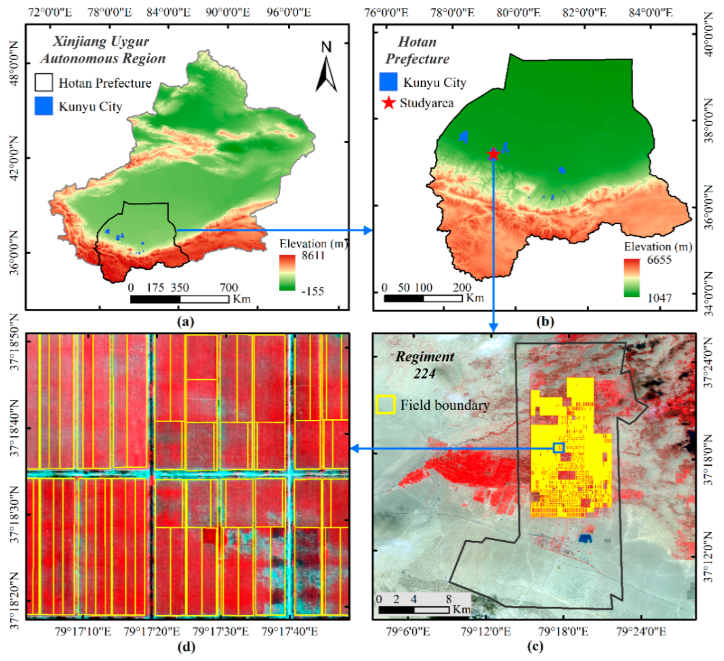
2.1. Study Area

The study area is located in Regiment 224, the Xinjiang Production and Construction Corps 14th Division in Kunyu City, the southern edge of the Taklimakan near Pishan County and Moyu County, Hotan Prefecture, Xinjiang, China (Figure 1). The study area is approximately 234.75 km2 with a north-south average length of 24.0 km and an east-west average width of 9.2km. The study area has abundant solar energy and large temperature differences between day and night, which is conducive to the accumulation of jujube sugar, so it is the representative area for jujube cultivation in Xinjiang.
The regiment started planting jujube in 2003. As of 2019, the area of jujube planted was about 90 km2, accounting for 72% of the agricultural land and 83% of the orchard land. However, the jujube industry is greatly affected by market risks and climate change. With the continuous expansion of jujube planting in the surrounding areas, the production of jujube exceeds demand. Especially by the end of 2014, the price of jujube began to drop sharply. In addition, in 2016, when the jujube in the study area was in the sugar-bearing period, it was affected by excessive rain, causing a substantial reduction in the production of jujube and serious losses for growers. Up to now, the price of jujube is still low, which makes growers reduce or even abandon the investment and management of jujube orchards.

2.2. Land Abandonment Process in Jujube

The ecological succession of an abandoned field consists of the gradual replacement of the crop by the wild vegetation of the area. During the first to the second years of abandonment, the jujube branches and leaves grow messy due to no pruning management. At the same time, wild vegetation such as reeds, suaeda salsa, inula, etc. gradually expands in the field. During the third to the fourth years of abandonment, jujube trees will gradually degenerate or even die due to lack of irrigation and increase of wild vegetation height and cover. Finally, the death of the trees can occur, and the wild vegetation will occupy the entire field. In addition, the study area has an arid climate and high ground evaporation, coupled with the sharp increase in water consumption due to the expansion of jujube cultivation, the phenomenon of secondary soil salinization occurred in some plots in 2006, with a trend of increasing year by year. To alleviate this problem, alkali draining ditches between some jujube orchards were built by the local government. Therefore, the alkali draining ditches were one of the important land types in the study area.
Three different types of fields were classified according to the cover types found in the study area (Figure 2): (a) In-production—these were fields with jujube productive cultivation, in which jujube occupied most of the surface; (b) Abandoned—these were abandoned fields with jujube trees and wild vegetation; (c) Alkali draining ditch—these were ditches used to drain saline-alkali water, which were surrounded by the same types of wild vegetation as abandoned fields.

2.3. Data and Processing

2.3.1. Remote Sensing Data

The Gaofen-1 (GF1) satellite, which was successfully launched on 26 April 2013, was the first satellite of the Chinese “High-Resolution Earth Observation Systems” and can provide multi-resolution (2, 8, and 16 m) data [14]. Currently, the GF1 satellite, the GF1 B/C/D satellite launched on 31 March 2018, and the Gaofen-6 (GF6) satellite launched on 2 June 2018 have realized on-orbit network operation. Their ability to monitor agriculture, forestry, grassland, and other resources has been greatly improved, which is of great significance to the precise management of crops. The data used in this study consisted of a time series of GF1 panchromatic and multispectral (PMS) imagery and GF6 PMS imagery from April to November of 2019. The specific image parameters are shown in Table 1.

2.3.2. Image Preprocessing

The flowchart of image processing is shown in Figure 3. Image preprocessing was based on ENVI 5.3. The Radiometric Calibration tool that can automatically read the metadata from the sensors listed above for calibration was used to obtain the radiance of the images, while the atmospheric correction was performed using the Fast Line-of-Site Atmospheric Analysis of Spectral Hypercube (FLAASH) tool. In addition, the ortho-rectification was performed based on the rational polynomial coefficient (RPC) files of the GF satellite image products. Then, the multispectral imagery with 2-m resolution was obtained by fusing the four multispectral bands with the panchromatic band with the NNDiffuse (nearest neighbor diffusion) Pan Sharpening method. The multi-temporal remote sensing images were well geo-referenced with good alignment.

2.3.3. Spectral Feature Extraction

VIs can quantify vegetation attributes by converting the reflectance of two or more spectral bands. In this study, five VIs were selected to obtain the differences between in-production fields, abandoned fields, and alkali draining ditches. The formulas for the VIs are presented in Table 2.
NDVI is one of the most common vegetation indices, which can reflect the comprehensive change in crop growth. However, it is easily disturbed by the soil reflectance when the canopy density is low, and it is easily saturated with dense vegetation. The soil-adjusted vegetation index (SAVI) can compensate for the influence of soil background while the enhanced vegetation index (EVI) can correct for the saturation effect and the ratio vegetation index (RVI) is more sensitive to vegetation greenness. In addition, the normalized difference water index (NDWI), which is sensitive to water content, can capture the moisture differences that may exist between alkali draining ditch, irrigated fields, and abandoned fields (non-irrigated).

2.3.4. Texture Feature Extraction

The grey-level co-occurrence matrix (GLCM) was first proposed by Haralick in 1973 [48], and it is one of the most common texture statistical analysis methods. It can calculate 14 texture features (TFs), and eight of them are commonly used in remote sensing, including mean, variance, homogeneity, contrast, dissimilarity, entropy, angular second moment, and correlation [49]. Among them, homogeneity, contrast, and dissimilarity are contrast-based, entropy and angular second moment are orderliness-based, and angular second moment represents the opposite of the entropy. In addition, contrast and dissimilarity as well as entropy and angular second moment are the conceptions corresponding to each other [32,42]. To reduce the correlation between TFs, mean, variance, contrast, entropy and correlation were chosen as the representative features in this study to distinguish the abandoned fields, in-production fields, and alkali draining ditches. Finally, the TFs were extracted based on the panchromatic bands of nine temporal images in ENVI 5.3. The formulas and descriptions for the TFs are presented in Table 3.

2.3.5. Field Sample Data

The ground truth data were collected during the field survey between 16 and 20 September 2019. A total of 227 fields was selected (79 abandoned fields, 63 alkali draining ditches, and 85 in-production fields). The dataset for each class was randomly divided into a training set and a validation set at a ratio of 3:2. Finally, 137 fields (48 abandoned fields, 38 alkali draining ditches, and 51 in-production fields) were selected for model training, and 90 fields (31 abandoned fields, 25 alkali draining ditches, and 34 in-production fields) were selected for model verification (Figure 4). In addition, we had collected 2019 cadastral data in vector format of the study area and used the data to obtain the field boundaries.

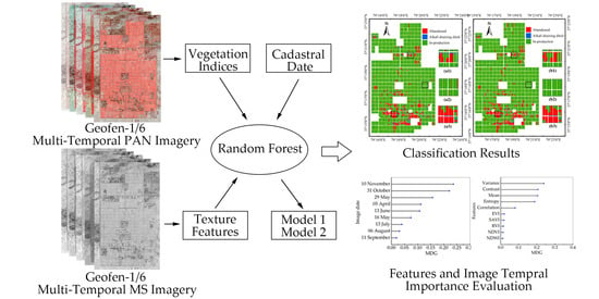
2.4. Random Forest Algorithm

RF [41] is an ensemble classifier based on a decision tree and combined with the Bagging method. It has higher classification accuracy and stronger generalization performance than a single decision tree and could handle well large and high dimensional data. In this research, nine temporal images were masked using a cadastral layer to define agricultural fields, and 10 features (5 VIs and 5 TFs) were calculated for the nine images. The multi-temporal single-band VI and TF images were then compiled into a 90-layer data cube for further analysis.
In the training stage of the RF classifier, the bootstrap method was used to randomly select training sample sets. Each training sample set could grow into a decision tree, and after the above sampling and tree building process was repeated N times, the RF classifier composed of N decision trees was finally established. In the classification stage, each decision tree made an independent judgment on the category of the new sample, and the classification results of all decision trees were summarized and the majority voting principle was used to output the final result.
The design of a decision tree requires the choice of an attribute selection measure and a pruning method. In this study, the Gini impurity was employed to find the best split and the best of the n features to use in that split, and the Mean Decrease in Gini (MDG) [13], which measures the average gain of purity by splits of a given variable, was used to rank the importance of the variables. Considering the randomness of the RF feature selection when establishing the decision trees, the variable importance ranking also has a certain degree of randomness; therefore, the modeling process was repeated five times and the average MDG of each variable was used as the basis for the final importance ranking.
The RF algorithm was applied using the RandomForestClassifier from the scikit-learn in Python (version 3.8.5, 2020). Two models were designed using field boundaries for classification. Firstly, each field was treated as a whole, and the average VIs and TFs were calculated as the features for each field, and then the fields were classified according to the features. This method is referred to as field-based classification (Model 1) in this study. Secondly, pixel-based classification was performed firstly, and then each field was classified following the most frequent pixel value criterion inside the field, which is referred to as pixel-based classification (Model 2). The mean of all the pixels in each training field was used for training in Model 1, while all pixels covered by the training fields were used for training in Model 2. The details of each model are shown in Table 4.
In general, the more decision trees there are in the RF classifier, the better the prediction, and accordingly, the longer the calculation time. Therefore, a trade-off between the classification accuracy and the time efficiency is necessary. Models 1 and 2 were trained and optimized with an increasing number of decision trees based on the training fields and pixels (Table 4), respectively. In this study, different numbers of trees from 10 to 200 were tested and the step size was 10 (Figure 5). We selected 50 decision trees for Model 1 and 80 decision trees for the Model to classify the jujube fields when considering both the classification accuracy and time efficiency.

2.5. Accuracy Assessment

In this research, the jujube fields are clearly defined units and the classification results of the two models are presented in the form of fields. Therefore, field-based accuracy assessment was carried out using the validation fields shown in Table 4. A confusion matrix is a commonly used accuracy evaluation method. According to this method, various accuracy assessment parameters were calculated [50], including overall accuracy (OA), Kappa coefficient, producer’s accuracy (PA), and user’s accuracy (UA).

3. Results

3.1. Classification Accuracy Assessment and Results Analysis

The accuracy assessment results based on Models 1 and 2 are shown in Table 5. The overall accuracy of the two models was 91.1% and 90.0%, respectively, and the respective Kappa coefficient was 0.866 and 0.848. The in-production class was accurately identified with a PA of 97.1% for both models, and a UA of 94.3% for Model 1, and 91.7% for Model 2. The PA and UA of the abandoned class of Model 1 were 83.9% and 92.9%, respectively, while those of Model 2 were 93.6% and 82.9%, respectively. In addition, the PA and UA of the alkali draining ditch class of Model 1 were 92.0% and 85.2%, respectively, while those of Model 2 were 76.0% and 100.0%, respectively. These results indicate that both models accurately identified in-production fields with excellent PA and UA. Model 1 correctly identified 83.9% of the abandoned fields, but Model 2 identified 93.6% of the class. On the other hand, 92.9% of the abandoned fields identified on the classification map by Model 1 actually belonged to the class, but only 82.9% of the abandoned fields identified on the map by Model 2 were actually abandoned fields. Clearly, Model 2 identified more abandoned fields correctly than Model 1, even though some of the alkali draining ditches were misclassified as abandoned fields by Model 2. The confusion of abandoned fields and alkali draining ditch fields occurred in the classification process. This was due to the fact the same wild vegetation species grew around the ditches and abandoned jujube orchards, and some of the ditches were in a dry state throughout the growing season. In addition, the result of the initial pixel-based classification with Model 2 showed that the OA and Kappa were 84.8% and 0.725, respectively, and the PA and UA of the three different categories were lower than those of Model 1 and Model 2. The result showed that due to the difference in vegetation growth within the field, the traditional pixel-based classification resulted in more misclassified land types than Model 1 and Model 2.
According to the cadastral data in 2019, the study area was divided into 5905 fields, covering an area of 9090.06 ha. The two classification models were applied to the study area. Table 6 compares the number of fields and areas classified as abandoned, alkali draining ditch, and in-production by each model. The classification results of the two models were largely similar. The estimated abandoned areas were slightly over 800 ha or approximately 9% of the total area, the in-production areas were about 8200 ha, and the alkali draining ditch fields accounted for less than 1% of the total area for both methods. Meanwhile, the number of abandoned fields detected by Model 1 was more than that detected by Model 2, but the corresponding areas were just opposite. More alkali draining ditch fields and areas were detected by Model 1 than Model 2.
Figure 6 shows the distributions of the abandoned fields based on Models 1 and 2. It can be seen that the spatial distributions of the abandoned fields detected by both models (such as Figure 6(a3,b3)) were similar, which illustrates that there are more abandoned fields in the south and fewer in the central and northern of the study area. The mixes of abandoned fields and alkali draining ditch fields were also reflected in the classification results of the whole study area. As shown in Figure 6(a1,b1), some fields that were classified as alkali draining ditches by Model 1 were classified as abandoned fields by Model 2. In addition, some of the small fields near the roads were classified as the abandoned category (Figure 6(a1)) by Model 1, while these fields were classified as the in-production category (Figure 6(b1)) by Model 2. Therefore, the abandoned fields detected by Model 1 are greater in number and less in area than those detected by Model 2.

3.2. Classification Feature Importance Evaluation

In this study, MDG was used as the evaluation criterion of the importance of classification features. Figure 7 shows the ranking results of the top 20 important features based on the two classification models. Figure 7a illustrates that the TFs of the images of 10 November, 31 October, 29 May, and 5 April had higher importance, and the VIs were not included in the top 20 important features. Figure 7b illustrates that the texture feature Mean of the images of 31 October, 10 November, and 5 April were particularly important, followed by VIs such as EVI, SAVI, NDVI, NDWI, and RVI.
Figure 8 shows the comprehensive ranking results of the importance of each feature of the nine temporal images based on the two models. The results illustrate that the importance of TFs was significantly higher than that of VIs, and all VIs were less important in the field-based classification, while Mean was the most important, followed by EVI, SAVI, NDWI, NDVI, RVI, and other TFs in the pixel-based classification.

3.3. Image Date Importance Evaluation

Figure 9 shows the results of image date importance evaluation based on the two models. The results indicate that 31 October and 10 November were the two most important dates for distinguishing abandoned, alkali draining ditch, and in-production fields in both models, followed by 5 April, 29 May, and 13 June, and the importance of 13 July, 6 August, and 11 September was the lowest.
To further analyze the impact of the image date importance on the classification results, the images were gradually added according to the ranking of the image date importance from low to high and from high to low, respectively, and were then classified using the two models as the image from each addition date was added. The changes in OA and Kappa with the additional images are shown in Figure 10.
It can be seen from Figure 10a,b that when the images were gradually added from low to high according to the date importance, the OA and Kappa coefficients for both models showed an overall upward trend. In addition, the OA and Kappa increased when the images of 29 May, 13 June, 6 August, and 31 October were added, while the OA and Kappa had no change when the images of May 16 and July 13 were added. According to the classification results of Model 1, OA and Kappa decreased slightly when the 5 April image was added, OA and Kappa reached the highest values when the image of 31 October was added, and the image of 10 November had no effect on OA and Kappa. For Model 2, OA and Kappa reached the highest values when all images were used for classification. Figure 10c,d, respectively show the changes of OA and Kappa when an image with the highest importance was added based on Model 1 and Model 2. A good classification result was achieved using the 10 November image alone based on Model 1. OA and Kappa increased slightly when the 13 June image was added, while these values decreased slightly when the 13th July image was added. The classification results were not affected by adding the other temporal images. For Model 2, the results were best when the images of 31 October, 10 November, 5 April, and 13 June were used together for classification. The addition of the 13 July image slightly lowered OA and Kappa, but adding the 6 August image improved these values. The addition of the images from the other dates had no obvious impact on the classification results.
The result showed that the OA and Kappa were low with only the 31 October and 10 November images for Model 2. To analyze the reason for this, Table 7 lists the classification accuracies generated by Model 2 as the images were gradually added from high to low based on their date importance. According to Table 7, the UA of abandoned fields and the PA of alkali draining ditch fields were very low with only the 31 October and 10 November images, because some of the alkali draining ditches were misclassified as abandoned fields by Model 2. Although the low UA for abandoned fields and low PA for the ditch fields significantly reduced the OA and Kappa for the 31 October and 10 November images, we found that Model 2 could correctly identify over 90% of the abandonment. 5 April and 13 June were in the sprouting period and the flowering period, respectively, for jujube, and the amount of irrigation increased greatly, therefore, the water surface area in the alkali draining ditch fields increased, which greatly improved the probability of the alkali draining ditches being correctly classified. In short, later October to early November can be an important period for abandoned jujube land detection, and using images from July to September alone will have certain challenges for identifying jujube abandoned fields.

4. Discussion

In this research, we demonstrated the feasibility of identifying abandoned jujube fields with high-resolution multi-temporal images combined with spectral features, texture features, and the RF algorithm. At present, the mainstream of the abandoned land research is concentrated on change detection in land-use types over large areas with MODIS images [8,9,10,51]. There is also some research on the mapping of small areas of abandoned farmland using high-resolution and/or medium-resolution satellite images [52,53]. The objects of this research are usually farmland in a broad sense, and there are still few studies on the abandonment of specific crops. Additionally, most of these studies focused on annual crops rather than perennial crops. The jujube abandoned land identification proposed in this study is different from the above research, and it is more similar to the identification of abandoned citrus lands [13]. Abandoned land identification of the study is based on the detection of its own physiological state changes and the detection of the succession vegetation of invading abandoned fields [54]. In addition, jujube trees have obvious phenological characteristics during the growing season [3]. Therefore, multi-temporal images were used as a strategy in this research to detect the jujube abandoned fields to achieve the best classification accuracy.
The technical scheme adopted in this study (a combination of image and cadastral data, spectral features, texture features, and classification methods) achieved good results in the detection of abandoned jujube fields. Firstly, this study employed high-resolution remote sensing images, which can improve the limitations of mapping small abandoned land to a certain extent [13]. Secondly, the method proposed in the study combined spectral and texture information to distinguish abandoned jujube fields, alkali draining ditches, and in-production fields, which made better use of the apparent differences among the cover types. Third, this study combined the cadastral vector data of the study area in the current year to obtain the boundaries of the fields and to ensure that these fields were independent units, which can alleviate to a certain extent the misclassification and the salt-and-pepper noise with the traditional pixel-based classification. In addition, both field-based and pixel-based classification methods according to field boundaries were used to identify the abandoned land in the research, and both methods achieved a high OA of 91.11% and 90.00%, respectively. The field-based classification method can greatly reduce the number of training samples and significantly improve computational efficiency. However, some studies have shown that classification based on plots may reduce the classification accuracy due to the reduction of training samples [23]. The reason for the better classification accuracy in this study may be partly related to the sufficient sample. Whether this method can achieve good results in other abandoned land or agricultural land classification needs to be determined based on specific conditions. In addition, the possibility that field area and field boundaries may change every year should also be considered for image classification based on field boundaries. It is usually effective to update the parcel or field boundaries with image segmentation and other methods [24], which need to be further explored in the research of abandoned land detection.
The omission and commission errors should be considered with both classification approaches. For the field-based classification, the omission error of abandoned fields was 16.1%, and the commission error of alkali draining ditches was 14.8%, while the commission error of abandoned fields was 17.1%, and the omission error of alkali draining ditches was 24% in the pixel-based classification result. These relatively large errors were mainly due to the similarity of the wild vegetation growing in the alkali draining ditches and abandoned fields. The alkali draining ditch fields were mainly composed of water surface, bare soil, and wild vegetation similar to those in abandoned fields (Figure 2c). Moreover, some alkali draining ditches were in a dry state, making the phenological and apparent differences of the two types of land smaller. Therefore, in future research, it is necessary to consider the subtle differences between the two types of land and explore the features that are more suitable for distinguishing them.
The RF algorithm can handle a large amount of high-dimensional data and is widely used for variable importance ranking [41,55]. In this research, the algorithm was used to process the multi-layer data cube and evaluate the importance of the 90 variables. The results showed that there were differences in the importance of features for the two classification approaches, but overall, TFs were more important than VIs. The importance of all TFs was greatly higher than that of VIs in the field-based classification, while the texture feature Mean was considered the most important variable followed by VIs in the pixel-based classification. This was because the differences in TFs were obvious in all the images across the growing season partly due to the spatial patterns of the trees, while the differences in VIs during a certain vegetation growth period may be small.
In addition, the result of the image date importance evaluation shows that 31 October and 10 November were the best dates for image classification. Using images only from July to September may pose a challenge to the identification of abandoned jujube fields. This is because the jujube trees have obvious phenological phenomena within one year [2]. Generally speaking, April is the germination period, while May and June are the flowering periods. July and August are the periods of rapid fruit growth, September and October are the fruit maturity period, and the deciduous period is in early November. The leaves of the jujube trees in the in-production plots gradually fall off from later October to early November, leaving the fruit on the trees, while the trees and wild vegetation on the abandoned fields enter the deciduous period earlier. Therefore, their TFs and VIs at this stage are quite different. However, during the period from July to September, jujube trees and other wild vegetation are in a period of vigorous growth. The NDVI and other VIs of abandoned fields are even higher than those of jujube trees of in-production fields. Therefore, it is difficult to separate the abandoned from the in-production fields during this period.
This study found that the jujube abandoned fields were mainly distributed in the southern part of the study area, showing a certain aggregation phenomenon. Most of these fields were close to alkali draining ditches, and the salinization was more serious. It can be inferred that the jujube abandonment was related to land salinization to some extent. During the field investigation, we learned that Regiment 224 was also actively investigating the abandoned land and the improvement of land salinization. The results of our research will provide a useful data source for their work. In addition, jujube trees are one of the most important economic crops in Xinjiang, and there are great similarities in the planting patterns and field divisions [3,4]. Several satellite imaging systems, such as Gaofen-1 wide field of view (WFV), Gaofen-6 WFV [56], and Sentinel-2 [57] with fine spatial, spectral, and temporal resolutions, have become freely available. Therefore, the next step of the research will be to evaluate these satellite images and different machine learning and deep learning methods to detect the abandoned jujube land over large areas, such as the jujube planting area in Hotan Prefecture.

5. Conclusions

In this study, we studied the jujube abandonment based on multi-temporal high-resolution images (GF1 and GF6 PMS) and RF algorithms. Both field-based and pixel-based classification approaches using field boundaries allowed the successful mapping of the abandonment of jujube fields. Field-based accuracy assessment confirmed the feasibility of the two classification methods. The overall OA (91.1%) and Kappa (0.866) of the field-based classification were slightly higher than those of the pixel-based classification (90.0% and 0.848), and the two methods produced similar spatial distributions of abandoned jujube fields. In addition, we evaluated the importance of multi-temporal VIs and TFs, and the results showed that the overall importance of TFs was higher than that of VIs. Furthermore, we assessed the importance of the multi-temporal images, and the results showed that 31 October and 10 November were the best dates for abandoned land detection, while the use of July, August, and September images presented certain challenges in the extraction of abandoned land. Our results suggested that when the field sample data is sufficient, a field-based classification can be selected for the extraction of the abandonment because that will greatly improve the calculation efficiency. At the same time, the methodology we used to identify abandoned land in this study can help us to have a deeper understanding of the management and land use of jujube orchards, and it will be beneficial for the local government to make timely adjustments to the abandonment and have the potential to be applied to other areas. Evaluating different satellite images and different classification methods to detect the abandonment of jujube fields is a work that needs further research.

Author Contributions

X.L. conceived and designed the experiment, collected the images and ground data, processed and analyzed the images, and drafted the manuscript. Q.Z., C.Y., and H.Z. guided the experimental design, participated in data collection, advised on data analysis, and revised the manuscript. P.W., J.T., and Y.T. were involved in the process of experiment design, data collection, or manuscript editing. All authors have read and agreed to the published version of the manuscript.

Funding

This research received financial support from the Science and Technology Project of Xinjiang Production and Construction Corps under Grant No. 2019AB002 and Hainan Provincial Department of Science and Technology under Grant No. ZDKJ2019006.

Data Availability Statement

Restrictions apply to the availability of Gaofen-1and Gaofen-6 data, and it is available from the funders by request.

Acknowledgments

The authors wish to thank Regiment 224 of the Xinjiang Production and Construction Corps 14th Division for the help in the collection of the ground data and field data. Thanks are also extended to the China Centre for Resources Satellite Data and Application for the series of Gaofen imagery. Mention of a commercial product is solely to provide specific information and should not be construed as a product endorsement by the authors or the institutions with which the authors are affiliated.

Conflicts of Interest

The authors declare no conflict of interest.

References

  1. Wang, R.; Ding, S.; Zhao, D.; Wang, Z.; Wu, J.; Hu, X. Effect of dehydration methods on antioxidant activities, phenolic contents, cyclic nucleotides, and volatiles of jujube fruits. Food Sci. Biotechnol. 2016, 25, 137–143. [Google Scholar] [CrossRef]
  2. Gao, Q.-H.; Wu, C.-S.; Wang, M. The Jujube (Ziziphus Jujuba Mill.) Fruit: A Review of Current Knowledge of Fruit Composition and Health Benefits. J. Agric. Food Chem. 2013, 61, 3351–3363. [Google Scholar] [CrossRef] [PubMed]
  3. Bai, T.; Zhang, N.; Mercatoris, B.; Chen, Y. Jujube yield prediction method combining Landsat 8 Vegetation Index and the phenological length. Comput. Electron. Agric. 2019, 162, 1011–1027. [Google Scholar] [CrossRef]
  4. Bai, T.-C.; Wang, T.; Zhang, N.-N.; Chen, Y.-Q.; Mercatoris, B. Growth simulation and yield prediction for perennial jujube fruit tree by integrating age into the WOFOST model. J. Integr. Agric. 2020, 19, 721–734. [Google Scholar] [CrossRef]
  5. Yoon, H.; Kim, S. Detecting abandoned farmland using harmonic analysis and machine learning. ISPRS J. Photogramm. Remote Sens. 2020, 166, 201–212. [Google Scholar] [CrossRef]
  6. Wu, M.; Hu, Y.; Wang, H.; Liu, G.; Yang, L. Remote sensing extraction and feature analysis of abandoned farmland in hilly and mountainous areas: A case study of Xingning, Guangdong. Remote Sens. Appl. Soc. Environ. 2020, 20, 100403. [Google Scholar] [CrossRef]
  7. Löw, F.; Prishchepov, A.V.; Waldner, F.; Dubovyk, O.; Akramkhanov, A.; Biradar, C.; Lamers, J.P.A. Mapping Cropland Abandonment in the Aral Sea Basin with MODIS Time Series. Remote Sens. 2018, 10, 159. [Google Scholar] [CrossRef] [Green Version]
  8. Estel, S.; Kuemmerle, T.; Alcántara, C.; Levers, C.; Prishchepov, A.V.; Hostert, P. Mapping farmland abandonment and recultivation across Europe using MODIS NDVI time series. Remote Sens. Environ. 2015, 163, 312–325. [Google Scholar] [CrossRef]
  9. Alcantara, C.; Kuemmerle, T.; Baumann, M.; Bragina, E.V.; Griffiths, P.; Hostert, P.; Knorn, J.; Müller, D.; Prishchepov, A.V.; Schierhorn, F.; et al. Mapping the extent of abandoned farmland in Central and Eastern Europe using MODIS time series satellite data. Environ. Res. Lett. 2013, 8, 035035. [Google Scholar] [CrossRef]
  10. Zhu, X.; Xiao, G.; Zhang, D.; Guo, L. Mapping abandoned farmland in China using time series MODIS NDVI. Sci. Total Environ. 2021, 755, 142651. [Google Scholar] [CrossRef]
  11. Löw, F.; Fliemann, E.; Abdullaev, I.; Conrad, C.; Lamers, J.P. Mapping abandoned agricultural land in Kyzyl-Orda, Kazakhstan using satellite remote sensing. Appl. Geogr. 2015, 62, 377–390. [Google Scholar] [CrossRef]
  12. Yusoff, N.M.; Muharam, F.M.; Khairunniza-Bejo, S. Towards the use of remote-sensing data for monitoring of abandoned oil palm lands in Malaysia: A semi-automatic approach. Int. J. Remote Sens. 2016, 38, 432–449. [Google Scholar] [CrossRef]
  13. Morell-Monzó, S.; Estornell, J.; Sebastiá-Frasquet, M. Comparison of Sentinel-2 and high-resolution imagery for mapping land abandonment in fragmented areas. Remote Sens. Basel. 2020, 12, 2062. [Google Scholar] [CrossRef]
  14. Zhou, Q.-B.; Yu, Q.-Y.; Liu, J.; Wu, W.-B.; Tang, H.-J. Perspective of Chinese GF-1 high-resolution satellite data in agricultural remote sensing monitoring. J. Integr. Agric. 2017, 16, 242–251. [Google Scholar] [CrossRef]
  15. Chen, M.; Ke, Y.; Bai, J.; Li, P.; Lyu, M.; Gong, Z.; Zhou, D. Monitoring early stage invasion of exotic Spartina alterniflora using deep-learning super-resolution techniques based on multisource high-resolution satellite imagery: A case study in the Yellow River Delta, China. Int. J. Appl. Earth Obs. Geoinf. 2020, 92, 102180. [Google Scholar] [CrossRef]
  16. Zhang, D.; Pan, Y.; Zhang, J.; Hu, T.; Zhao, J.; Li, N.; Chen, Q. A generalized approach based on convolutional neural networks for large area cropland mapping at very high resolution. Remote Sens. Environ. 2020, 247, 111912. [Google Scholar] [CrossRef]
  17. Bruzzone, L.; Carlin, L. A multilevel context-based system for classification of very high spatial resolution images. IEEE Trans. Geosci. Remote Sens. 2006, 44, 2587–2600. [Google Scholar] [CrossRef] [Green Version]
  18. Prishchepov, A.V.; Radeloff, V.C.; Baumann, M.; Kuemmerle, T.; Müller, D. Effects of institutional changes on land use: Agricultural land abandonment during the transition from state-command to market-driven economies in post-Soviet Eastern Europe. Environ. Res. Lett. 2012, 7, 024021. [Google Scholar] [CrossRef]
  19. Lambin, E.F.; Meyfroidt, P. Global land use change, economic globalization, and the looming land scarcity. Proc. Natl. Acad. Sci. USA 2011, 108, 3465–3472. [Google Scholar] [CrossRef] [Green Version]
  20. Peña-Barragán, J.M.; Ngugi, M.K.; Plant, R.E.; Six, J. Object-based crop identification using multiple vegetation indices, textural features and crop phenology. Remote Sens. Environ. 2011, 115, 1301–1316. [Google Scholar] [CrossRef]
  21. Liu, C.; Shang, J.; Vachon, P.W.; McNairn, H. Multiyear Crop Monitoring Using Polarimetric RADARSAT-2 Data. IEEE Trans. Geosci. Remote Sens. 2012, 51, 2227–2240. [Google Scholar] [CrossRef]
  22. Blaschke, T. Object based image analysis for remote sensing. ISPRS J. Photogramm. Remote Sens. 2010, 65, 2–16. [Google Scholar] [CrossRef] [Green Version]
  23. Duro, D.C.; Franklin, S.E.; Dubé, M.G. A comparison of pixel-based and object-based image analysis with selected machine learning algorithms for the classification of agricultural landscapes using SPOT-5 HRG imagery. Remote Sens. Environ. 2012, 118, 259–272. [Google Scholar] [CrossRef]
  24. Kussul, N.; Lemoine, G.; Gallego, F.J.; Skakun, S.V.; Lavreniuk, M.; Shelestov, A.Y. Parcel-Based Crop Classification in Ukraine Using Landsat-8 Data and Sentinel-1A Data. IEEE J. Sel. Top. Appl. Earth Obs. Remote Sens. 2016, 9, 2500–2508. [Google Scholar] [CrossRef]
  25. Paredes-Gómez, V.; Gutiérrez, A.; Del Blanco, V.; Nafría, D.A. A Methodological Approach for Irrigation Detection in the Frame of Common Agricultural Policy Checks by Monitoring. Agronomy 2020, 10, 867. [Google Scholar] [CrossRef]
  26. Bruce, R.W.; Rajcan, I.; Sulik, J. Plot extraction from aerial imagery: A precision agriculture approach. Plant Phenome J. 2020, 3, 3. [Google Scholar] [CrossRef] [Green Version]
  27. Aplin, P.; Atkinson, P.M.; Curran, P.J. Fine Spatial Resolution Simulated Satellite Sensor Imagery for Land Cover Mapping in the United Kingdom. Remote Sens. Environ. 1999, 68, 206–216. [Google Scholar] [CrossRef]
  28. Arikan, M. Parcel based crop mapping through multi-temporal masking classification of Landsat 7 images in Karacabey, Turkey. Int. Arch. Photogramm. Remote Sens. Spat. Inf. Sci. 2004, 34, 12–23. [Google Scholar]
  29. Blaes, X.; Vanhalle, L.; Defourny, P. Efficiency of crop identification based on optical and SAR image time series. Remote Sens. Environ. 2005, 96, 352–365. [Google Scholar] [CrossRef]
  30. Yang, S.; Gu, L.; Li, X.; Jiang, T.; Ren, R. Crop Classification Method Based on Optimal Feature Selection and Hybrid CNN-RF Networks for Multi-Temporal Remote Sensing Imagery. Remote Sens. 2020, 12, 3119. [Google Scholar] [CrossRef]
  31. Guo, A.; Huang, W.; Ye, H.; Dong, Y.; Ma, H.; Ren, Y.; Ruan, C. Identification of Wheat Yellow Rust Using Spectral and Texture Features of Hyperspectral Images. Remote Sens. 2020, 12, 1419. [Google Scholar] [CrossRef]
  32. Kim, H.-O.; Yeom, J.-M. Effect of red-edge and texture features for object-based paddy rice crop classification using RapidEye multi-spectral satellite image data. Int. J. Remote Sens. 2014, 35, 1–23. [Google Scholar] [CrossRef]
  33. Bhuyar, N.; Acharya, S.; Theng, D. Crop Classification with Multi-Temporal Satellite Image Data. Int. J. Eng. Res. 2020, 9. [Google Scholar] [CrossRef]
  34. Jakubauskas, M.E.; LeGates, D.R.; Kastens, J.H. Crop identification using harmonic analysis of time-series AVHRR NDVI data. Comput. Electron. Agric. 2002, 37, 127–139. [Google Scholar] [CrossRef]
  35. Gilbertson, J.K.; Kemp, J.; van Niekerk, A. Effect of pan-sharpening multi-temporal Landsat 8 imagery for crop type differentiation using different classification techniques. Comput. Electron. Agric. 2017, 134, 151–159. [Google Scholar] [CrossRef] [Green Version]
  36. Zhang, H.; Kang, J.; Xu, X.; Zhang, L. Accessing the temporal and spectral features in crop type mapping using multi-temporal Sentinel-2 imagery: A case study of Yi’an County, Heilongjiang province, China. Comput. Electron. Agric. 2020, 176, 105618. [Google Scholar] [CrossRef]
  37. Yusoff, N.M.; Muharam, F.M. The Use of Multi-Temporal Landsat Imageries in Detecting Seasonal Crop Abandonment. Remote Sens. 2015, 7, 11974–11991. [Google Scholar] [CrossRef] [Green Version]
  38. Breiman, L. Random Forests. Mach. Learn. 2001, 45, 5–32. [Google Scholar] [CrossRef] [Green Version]
  39. Li, X.; Yang, C.; Huang, W.; Tang, J.; Tian, Y.; Zhang, Q. Identification of Cotton Root Rot by Multifeature Selection from Sentinel-2 Images Using Random Forest. Remote Sens. 2020, 12, 3504. [Google Scholar] [CrossRef]
  40. Belgiu, M.; Drăguţ, L. Random forest in remote sensing: A review of applications and future directions. ISPRS J. Photogramm. Remote Sens. 2016, 114, 24–31. [Google Scholar] [CrossRef]
  41. Fletcher, R.S.; Reddy, K.N. Random forest and leaf multispectral reflectance data to differentiate three soybean varieties from two pigweeds. Comput. Electron. Agric. 2016, 128, 199–206. [Google Scholar] [CrossRef]
  42. Zhang, L.; Liu, Z.; Ren, T.; Liu, D.; Ma, Z.; Tong, L.; Zhang, C.; Zhou, T.; Zhang, X.; Li, S. Identification of Seed Maize Fields With High Spatial Resolution and Multiple Spectral Remote Sensing Using Random Forest Classifier. Remote Sens. 2020, 12, 362. [Google Scholar] [CrossRef] [Green Version]
  43. Rouse, J.W.; Haas, R.H.; Schell, J.A.; Deering, D.W. Monitoring Vegetation Systems in the Great Plains with Erts. NASA Spéc. Publ. 1974, 351, 309. [Google Scholar]
  44. Huete, A. A soil-adjusted vegetation index (SAVI). Remote Sens. Environ. 1988, 25, 295–309. [Google Scholar] [CrossRef]
  45. Huete, A.; Didan, K.; Miura, T.; Rodriguez, E.P.; Gao, X.; Ferreira, L.G. Overview of the radiometric and biophysical performance of the MODIS vegetation indices. Remote Sens. Environ. 2002, 83, 195–213. [Google Scholar] [CrossRef]
  46. Zhang, L.; Liu, Z.; Liu, D.; Xiong, Q.; Yang, N.; Ren, T.; Zhang, C.; Zhang, X.; Li, S. Crop Mapping Based on Historical Samples and New Training Samples Generation in Heilongjiang Province, China. Sustainability 2019, 11, 5052. [Google Scholar] [CrossRef] [Green Version]
  47. Birth, G.S.; McVey, G.R. Measuring the Color of Growing Turf with a Reflectance Spectrophotometer 1. Agron. J. 1968, 60, 640–643. [Google Scholar] [CrossRef]
  48. Haralick, R.M.; Shanmugam, K.; Dinstein, I. Textural Features for Image Classification. IEEE Trans. Syst. Man Cybern. 1973, 3, 610–621. [Google Scholar] [CrossRef] [Green Version]
  49. Murray, H.; Lucieer, A.; Williams, R. Texture-based classification of sub-Antarctic vegetation communities on Heard Island. Int. J. Appl. Earth Obs. Geoinf. 2010, 12, 138–149. [Google Scholar] [CrossRef]
  50. Foody, G.M. Status of land cover classification accuracy assessment. Remote Sens. Environ. 2002, 80, 185–201. [Google Scholar] [CrossRef]
  51. Alcantara, C.; Kuemmerle, T.; Prishchepov, A.V.; Radeloff, V.C. Mapping abandoned agriculture with multi-temporal MODIS satellite data. Remote Sens. Environ. 2012, 124, 334–347. [Google Scholar] [CrossRef]
  52. Kuemmerle, T.; Hostert, P.; Radeloff, V.C.; Van Der Linden, S.; Perzanowski, K.; Kruhlov, I. Cross-border Comparison of Post-socialist Farmland Abandonment in the Carpathians. Ecosystems 2008, 11, 614–628. [Google Scholar] [CrossRef]
  53. Milenov, P.; Vassilev, V.; Vassileva, A.; Radkov, R.; Samoungi, V.; Dimitrov, Z.; Vichev, N. Monitoring of the risk of farmland abandonment as an efficient tool to assess the environmental and socio-economic impact of the Common Agriculture Policy. Int. J. Appl. Earth Obs. Geoinf. 2014, 32, 218–227. [Google Scholar] [CrossRef]
  54. Szostak, M.; Hawryło, P.; Piela, D. Using of Sentinel-2 images for automation of the forest succession detection. Eur. J. Remote Sens. 2018, 51, 142–149. [Google Scholar] [CrossRef]
  55. Zheng, Q.; Huang, W.; Cui, X.; Shi, Y.; Liu, L. New Spectral Index for Detecting Wheat Yellow Rust Using Sentinel-2 Multispectral Imagery. Sensors 2018, 18, 868. [Google Scholar] [CrossRef] [Green Version]
  56. Wang, M.; Cheng, Y.; Guo, B.; Jin, S. Parameters determination and sensor correction method based on virtual CMOS with distortion for the GaoFen6 WFV camera. ISPRS J. Photogramm. Remote Sens. 2019, 156, 51–62. [Google Scholar] [CrossRef]
  57. Gomez, V.P.; Del Blanco Medina, V.; Bengoa, J.L.; Nafría García, D.A. Accuracy Assessment of a 122 Classes Land Cover Map Based on Sentinel-2, Landsat 8 and Deimos-1 Images and Ancillary Data. In Proceedings of the IGARSS 2018—2018 IEEE International Geoscience and Remote Sensing Symposium, Valencia, Spain, 22–27 July 2018; pp. 5453–5456. [Google Scholar] [CrossRef]
Figure 1. Location of the study area. (a) Xinjiang Uygur Autonomous; (b) Hotan Prefecture; (c) Regiment 224 and GF6 color-infrared (CIR) composite image; (d) zoomed-in jujube fields.
Remotesensing 13 00801 g001
Figure 2. Three types of jujube fields: (a) in-production field; (b) abandoned field; and (c) alkali draining ditch.
Remotesensing 13 00801 g002
Figure 3. Flowchart of image processing.
Remotesensing 13 00801 g003
Figure 4. Location of ground surveyed fields in September 2019.
Remotesensing 13 00801 g004
Figure 5. The convergence of the accuracy of (a) Model 1 and (b) Model 2. The models were trained with an increasing number of decision trees, and the accuracy of classification was evaluated from the field-based (Model 1) and pixel-based (Model 2) classification, respectively.
Remotesensing 13 00801 g005
Figure 6. Land abandonment maps generated by (a) Model 1 and (b) Model 2 for the study area and the zoomed-in rectangle scenes (a1)–(a3) and (b1)–(b3) for the areas marked on the maps are shown at the right.
Remotesensing 13 00801 g006
Figure 7. The top 20 important features according to Mean Decrease in Gini. (a) Model 1 and (b) Model 2.
Remotesensing 13 00801 g007
Figure 8. Comprehensive importance of each feature of nine temporal images. (a) Model 1 and (b) Model 2.
Remotesensing 13 00801 g008
Figure 9. Importance of image dates. (a) Model 1 and (b) Model 2.
Remotesensing 13 00801 g009
Figure 10. The changes in overall accuracy (OA) and Kappa coefficient (Kappa) as the images were added. (a) Model 1, the images were gradually added from low to high of date importance; (b) Model 2, the images were gradually added from low to high of date importance; (c) Model 1, the image were gradually added from high to low of date importance; (d) Model 2, the image were gradually added from high to low of date importance.
Remotesensing 13 00801 g010aRemotesensing 13 00801 g010b
Table 1. Specifications for GaoFen-1 (GF1) and GaoFen-6 (GF6) satellites.
Global Observation
Cycle
Repeat
Observation Cycle
Wavelength (nm)Spatial Resolution (m)Image Dates in 2019
(Day Month)
GF1,
GF1 B/C/D
41 days4 daysPAN: 450–900
Blue: 450–520
Green: 520–590
Red: 630–690
Infrared: 770–890
PAN: 2
MS: 8
29 May, 13 June, 13 July, 11 September,
10 November
GF641 days4 daysPAN: 450–900
Blue: 450–520
Green: 520–600
Red: 630–690
Infrared:760–900
PAN: 2
MS: 8
05 April, 16 May, 06 August, 31 October
Note: PAN = panchromatic band and MS = multispectral bands.
Table 2. Vegetation indices (VIs) were used for the identification of abandoned jujube fields in this study.
Spectral IndexCalculation FormulaRelated ToReference
Normalized difference vegetation index (NDVI) ( N I R R ) ( N I R + R ) Vegetation status,
canopy structure
[43]
Soil-adjusted vegetation index (SAVI) 1.5 × ( N I R R ) ( N I R + R + 0.5 ) Vegetation status,
soil background
[44]
Enhance vegetation index (EVI) 2.5 × ( N I R R ) ( N I R + 6 R 7.5 B + 1 ) Vegetation status,
canopy structure
[45]
Normalized difference water index (NDWI) ( G N I R ) ( G + N I R ) Water content[46]
Ratio vegetation index (RVI) N I R / R Vegetation status,
canopy structure,
leaf pigments
[47]
Table 3. Texture Features (TFs) were used for the identification of abandoned jujube fields in this study.
TextureCalculation FormulaDescription
Mean x , y = 1 G x P ( x , y ) The average grey level of all pixels in the matrix.
Variance x = 1 G y = 1 G ( x u ) 2 P ( x , y ) The rate of change of the pixels’ values.
Contrast x = 1 G y = 1 G ( x y ) 2 P ( x , y ) The local variations in the matrix.
Entropy x = 1 G y = 1 G P ( x , y ) l o g P ( x , y ) The level of disorder in the matrix.
Correlation x = 1 G y = 1 G ( x y ) ( y x ) P ( x , y ) V A R x V A R y The measurement of image linearity among the pixels.
Note: In the equations, x and y represent the row number and column number of the image, respectively; P ( x , y ) represents the relative frequency of two neighboring pixels.
Table 4. Summary of the parameters used in each classification model.
Classification Field TypeInput VariablesTraining SamplesValidation Samples
FieldsPixelsFields
Model 1Abandoned9048226,58931
Alkali Draining Ditch3844,31525
In-production51272,68534
Model 2Abandoned9048226,58931
Alkali Draining Ditch3844,31525
In-production51272,68534
Table 5. Confusion matrices generated by classification Models 1 and 2 for the validation fields.
Classification Field TypeGround-Truth Class (Field)
AbandonedAlkali Draining DitchIn-ProductionTotalUA
(%)
Model 1 OA: 91.1% Kappa: 0.866
Abandoned26202892.9%
Alkali Draining Ditch32312785.2%
In-production20333594.3%
Total31253490
PA (%)83.9%92.0%97.1%
Model 2 OA: 90.0% Kappa: 0.848
Abandoned29513582.9%
Alkali Draining Ditch019019100.0%
In-production21333691.7%
Total31253490
PA (%)93.6%76.0%97.1%
Ground-Truth Class (Pixel)
Traditional Pixel-Based Classification OA: 84.8% Kappa: 0.725
Abandoned195,71414,33633,949243,99980.2%
Alkali Draining Ditch766223,050634637,05962.2%
In-production23,0855005287,150315,24091.1%
Total229,36542,948323,985596,298
PA (%)85.3%53.7%88.6%
Note: OA = overall accuracy, PA = producer’s accuracy, UA = user’s accuracy, and Kappa = Kappa coefficient.
Table 6. Estimated number of fields and areas from the classification results of Models 1 and 2.
Classification Field TypeModel 1Model 2
Number of FieldsAreaNumber of FieldsArea
/ha%/ha%
Abandoned 609806.098.87587828.219.11
Alkali Draining Ditch22678.610.8614547.920.53
In-production 50708205.3690.2751738213.9390.36
Total59059090.0610059059090.06100.00
Table 7. Classification accuracies were generated by Model 2 as images were gradually added from high to low based on their date importance.
Image
Date
AbandonedAlkali Draining DitchIn-ProductionOA
(%)
Kappa
PA (%)UA (%)PA (%)UA (%)PA (%)UA (%)
31 October93.660.432.0100.091.291.275.662.329
10 November90.363.640.0100.094.188.977.865.792
05 April93.678.468.0100.097.191.787.881.335
13 June93.682.976.0100.097.191.790.084.763
29 May93.682.976.0100.097.191.790.084.763
16 May93.682.976.0100.097.191.790.084.763
13 July93.680.672.0100.097.191.788.983.051
06 August93.682.976.0100.097.191.790.084.763
11 September93.682.976.0100.097.191.790.084.763
Note: OA = overall accuracy, PA = producer’s accuracy, UA = user’s accuracy, and Kappa = Kappa coefficient.
Publisher’s Note: MDPI stays neutral with regard to jurisdictional claims in published maps and institutional affiliations.

