
Generative Adversarial Learning in YUV Color Space for Thin Cloud Removal on Satellite Imagery


1
School of Electronic, Electrical and Communication Engineering, University of Chinese Academy of Sciences, Beijing 101408, China
2
Aerospace Information Research Institute, Chinese Academy of Sciences, Beijing 100190, China
3
Key Laboratory of Technology in Geo-Spatial Information Processing and Application System, Chinese Academy of Sciences, Beijing 100190, China
*
Author to whom correspondence should be addressed.
Remote Sens. 2021, 13(6), 1079; https://doi.org/10.3390/rs13061079
Submission received: 28 January 2021
/
Revised: 27 February 2021
/
Accepted: 5 March 2021
/
Published: 12 March 2021
(This article belongs to the Special Issue Artificial Intelligence Algorithm for Remote Sensing Imagery Processing)
Abstract
:Clouds are one of the most serious disturbances when using satellite imagery for ground observations. The semi-translucent nature of thin clouds provides the possibility of 2D ground scene reconstruction based on a single satellite image. In this paper, we propose an effective framework for thin cloud removal involving two aspects: a network architecture and a training strategy. For the network architecture, a Wasserstein generative adversarial network (WGAN) in YUV color space called YUV-GAN is proposed. Unlike most existing approaches in RGB color space, our method performs end-to-end thin cloud removal by learning luminance and chroma components independently, which is efficient at reducing the number of unrecoverable bright and dark pixels. To preserve more detailed features, the generator adopts a residual encoding–decoding network without down-sampling and up-sampling layers, which effectively competes with a residual discriminator, encouraging the accuracy of scene identification. For the training strategy, a transfer-learning-based method was applied. Instead of using either simulated or scarce real data to train the deep network, adequate simulated pairs were used to train the YUV-GAN at first. Then, pre-trained convolutional layers were optimized by real pairs to encourage the applicability of the model to real cloudy images. Qualitative and quantitative results on RICE1 and Sentinel-2A datasets confirmed that our YUV-GAN achieved state-of-the-art performance compared with other approaches. Additionally, our method combining the YUV-GAN with a transfer-learning-based training strategy led to better performance in the case of scarce training data.
1. Introduction
With the rapid development of remote sensing technology, high-resolution satellite images are being widely used in resource surveys, environmental monitoring, and vegetation management [1,2]. However, nearly 67% of the earth’s surface is covered by clouds [3], which reduces the availability of satellite images greatly. To be specific, thick clouds block the ground in the form of opaque “white blocks”, resulting in local information loss of ground targets. Thin clouds cover nearly the entirety of satellite images in the form of semi-translucent “white gauze”, which causes changes of spectral information and the blurring of ground features. Therefore, cloud removal is of great significance for improving the availability of high-resolution satellite images.
Thick and thin clouds result in different applications being used on the images. In satellite images polluted by thick clouds, more attention is paid to detecting cloud masks, which essentially represent a dichotomy between cloud and non-cloud pixels. Promoted by advanced computer vision methods [4,5,6,7], the accuracy of thick cloud detection is constantly being improved, but these methods [8,9,10,11] are not applicable to detecting semi-translucent thin clouds. Furthermore, the restoration of areas on the ground occluded by thick clouds is not considered.
As far as thin cloud removal goes, suppressing thin cloud components from cloudy pixels and then restoring the critical information of ground targets, such as colors and textures, provide the possibility of cloud-covered satellite images for ground observation tasks. In this paper, we propose a generative adversarial network in YUV color space and a training strategy utilizing both real and simulated data for thin cloud removal. The main contributions of this work are reflected in the following:
- The reconstruction of cloud-free images was conducted in YUV color space, which is efficient at reducing the number of unrecoverable bright and dark pixels without increasing the complexity of the algorithm.
- A residual symmetrical encoding–decoding architecture, without down-sampling and up-sampling layers, was used as the generator to recover detailed information. A mixed loss function combining loss and adversarial loss in YUV color space was employed to guide model training, which further improved the effectiveness of detailed reconstruction and the accuracy of scene recognition.
- We conducted the first study of transfer learning upon simulated and real data for thin cloud removal. Our results show that a network initialized with simulated data and then optimized by real data has an advantage over a network trained only with scarce real data.
- Both the public benchmark for thin cloud removal RICE1 and self-constructed Sentinel-2A datasets were used to verify the effectiveness of the proposed method by ablation study. Moreover, we demonstrate that the proposed method outperforms one traditional and two deep learning-based approaches based on quantitative indexes and qualitative effects.
2. Related Works
A brief overview of typical works on thin cloud removal is provided in Section 2.1. Moreover, we introduce previous studies about image reconstruction in different color spaces in Section 2.2, and present a short introduction about transferring knowledge to scarce target data in Section 2.3.
2.1. Typical Thin Cloud Removal Methods
According to different processing means, existing thin cloud removal methods are mainly divided into frequency characteristic-based [12,13], spatial characteristic-based [14,15,16], spectral characteristic-based [17,18], and image transformation-based methods [19,20,21,22]. In addition, in order to substitute cloud-contaminated pixels with real cloud-free observations, multitemporal approaches [23,24] are applied widely, but these approaches need to exploit a series of multitemporal quantitative products, causing the acquisition of data to be expensive. The dark channel prior (DCP) method [16] deriving from haze removal is an effective spatial characteristic-based approach, which can achieve thin cloud removal because the illumination component of clouds is highly correlated with that of haze [25].
Compared with the aforementioned traditional methods, deep convolutional neural network (CNN)-based methods automatically learn features from datasets and achieve impressive performance in thin cloud removal. Conditional generative adversarial net (cGAN) [26] was directly applied in [27] to accomplish cloud removal on the Remote sensing Image Cloud Removing dataset (RICE) [28] with various landforms. Enomoto et al. [29] designed multispectral conditional generative adversarial net (McGAN), which extends the input of cGAN by adding a near infrared (NIR) image concatenated with red, green, and blue (RGB) images in a new channel. Grohnfeldt et al. [30] and Meraner et al. [31] used synthetic aperture radar (SAR) data as additional information. Cloud-GAN [32] contains two generators to realize bidirectional mapping between the cloudy and cloud-free images. In order to strengthen the constraint of prior information on the model, introducing the irradiance transmission model of cloudy images into the network was considered. Zou et al. [33] re-examined cloud detection and removal as a mixed energy separation process between foreground and background images. Unfortunately, their architecture is more suitable for detecting the masks of thick clouds, while real thin cloud pixels are easily misjudged as background pixels. To reduce the dependence on paired images, a semi-supervised method CR-GAN-PM [34] is proposed, which mainly involves two steps: the first step is to decompose cloud-free background layers and cloud distortion layers from the input images utilizing GANs; the second step is to reconstruct the input images by putting those layers into the redefined physical model of cloud distortion.
The above-mentioned deep CNN-based thin cloud removal methods suffer from some deficiencies. From the perspective of network architecture, details of the image are easily corrupted due to repeated down-sampling layers. To address this problem, Li et al. [35] proposed a deep residual symmetrical concatenation network (RSC-Net) without down-sampling and up-sampling operations to realize end-to-end thin cloud removal. The RSC-Net is an encoding-decoding framework consisting of multiple residual convolutional and deconvolutional blocks, thereby better preserving the details of images. However, the loss applied in RSC-Net is likely to cause image blurring [36,37]. Besides, existing networks including RSC-Net are all performed in RGB color space, in which the characteristic of clouds in each channel is significantly different because the light is scattered unequally in each wavelength when passing through clouds [38]. Once the network predicts the cloud component in a certain channel incorrectly, it is prone to cause color distortion, especially for bright and dark pixels.
Another deficiency of the present approaches is that the training set is limited to either simulated or real data. In [29,30], the networks remove thin clouds exclusively with simulated image pairs, however, simulated clouds of that kind are significantly different from actual clouds seen in visible light images. Considering the applicability of models to real cloudy images, networks in [27,32,33,34,35] are trained with real image pairs. Actually, real data acquisition is herculean and costly, and the reason has two folds. On the one hand, it is impractical to capture truly paired cloud-free and corresponding cloudy images of the same scene at consistent imaging conditions. On the other hand, only a few collected pairs meet the requirement that the imaging conditions of the paired images are similar, making the process of training set collection time-consuming. In a word, the limited paired data becomes a great handicap to develop robust algorithms on thin cloud removal.
2.2. Image Reconstruction in Different Color Spaces
The often-used color space is RGB in most image reconstruction methods. However, Jang et al. [39] indicated that the RGB color space does not consider the color perception of the human visual system. Then they proposed that it’s more effective in CIELAB color space to estimate high dynamic range images from low dynamic range images. Markchom et al. [40] explored an algorithm to remove clouds in HSI color space, which eliminates clouds only in the intensity channel to avoid the influence on the original color. Wu et al. [41] considered the transformation (or inverse transformation) between YUV and RGB is linear, realizing the remote sensing image colorization in YUV color space, which will not generate a nonlinear error in the processes of color transformation and prediction. Furthermore, the advantage of the YUV color space compared with the RGB color spaces is that it can represent luminance and chromatic information independently. All of these advantages inspire us to attempt the reconstruction of cloud-free images in YUV color space.
2.3. Transferring Knowledge to Scarce Target Data
Transfer learning provides a powerful way in training a deep network using scarce data, on the condition that the network has been initialized by a large-scale dataset. Many approaches [42,43,44] pre-train CNNs on ImageNet, a large-scale natural image dataset, and then fine-tune on target datasets relating to specific tasks. Considering the discrepancy of different domains, Huang et al. [45,46] suggested using SAR images to pre-train the model for SAR target recognition instead of solely applying optical ImageNet. Yosinski et al. [47] discussed how to experimentally quantify the generality versus specificity of neurons in each layer of a deep CNN. A final surprising result shows that transferring and then fine-tuning features, from almost any number of layers, results in networks generalizing better than those trained directly on the target dataset. Inspired by this, Malmgren-Hansen et al. [48] transferred the knowledge from the simulated SAR data to the real one by fine-tuning all parameters in the CNN with equal learning rate. In this paper, the transferability between simulated and real data will be explored, to improve the thin cloud removal performance of the model on truly cloudy images.
3. Method
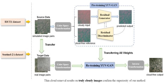
In this study, a workflow is proposed for thin cloud removal on satellite images. Methodologically, a YUV-GAN network architecture restoring cloud-free images in YUV color space and a training strategy based on transfer learning are proposed to remove thin clouds of real cloudy images. Figure 1 shows the overall framework of our method. The simulated image pairs as source data and real image pairs as target data are pre-processed by the color space transformation operation into images in YUV color space. The step of initializing the network parameters is then conducted by pre-training the YUV-GAN on sufficient simulated pairs, thereby avoiding collecting a large number of real training pairs. Subsequently, all parameters in the pre-trained model are transferred and the network is re-trained on scarce real pairs for real thin cloud removal. Finally, cloud-free images in RGB color space can be obtained by the post-processing Inverse Transformation operation. In the following, we will describe the proposed method in detail.
3.1. Color Space Transformation and Inverse Transformation
Thin cloud removal is a task sensitive to luminance and chromaticity. We attempted using RSC-Net [35] to remove thin clouds from cloudy images with some bright and dark pixels. Three-channel values of a bright pixel approximate 255, and those values of a dark pixel approximate 0. Figure 2 shows the failures of RSC-Net when predicting bright and dark pixels. We attribute the failures of recovering bright and dark pixels to luminance and chromatic information not independent of each other in R, G, and B channels. When the luminance and chromatic information of thin clouds in any channel cannot be accurately predicted, the pixels will have serious color deviations. In contrast, in YUV color space, the Y channel indicates luminance, and the U and V channels indicate chromatic information. Thus, the YUV color space is more suitable for recovering cloud-free images, as the luminance can change independently without affecting the chromatic information. For this reason, our method is implemented in YUV color space. RGB values can be transformed into YUV color space that considers color sensitivity through Equation (1). Additionally, YUV values can be transformed inversely into RGB color space through Equation (2) [41].
3.2. Architecture of YUV-GAN
The architecture enhances the quality of reconstructed cloud-free images via WGAN [49]. Residual blocks [50] are done in each layer of the generator and discriminator to replace all conventional convolution and deconvolution operations. The main advantage of the residual block is that the gradient of the former layer can be directly added into the latter layer, so there is no gradient dispersion or explosion when the network is going deeper. Figure 3 shows the architecture of the residual block. The kernel size of each convolution layer is 3 × 3, and each of them is followed by a Batch Normalization(BN) layer. Besides, the rectified linear unit (ReLU), chosen as the activation function, is adopted behind the first BN layer.
The generator in our work is based on a residual encoding–decoding architecture, as shown in Figure 4. There are no down-sampling and up-sampling layers, so detailed information in restoration can be better preserved. Both inputs and outputs of the generator are images of size 256 × 256 × 3 in YUV color space. On the encoding end, at first, convolution kernels with the size of 3 × 3 are used to convert 3-channel images to 32 feature maps; next comes a ReLU. After that, each of the five convolutional residual blocks produces 32 feature maps as outputs. The corresponding decoding end employs five deconvolutional residual blocks; each of them takes 64 feature maps as inputs and produces 32 feature maps as outputs; 32 feature maps copied from the symmetrical convolution layer constitute half of the deconvolutional inputs, and the other half are produced by the deconvolutional residual block in the last layer. At the end of the generator, convolution kernels with the size of 3 × 3 and a ReLU convert 32 feature maps to 3-channel images.
In order that the generator and discriminator can effectively optimize each other, the discriminator uses a residual neural network as depicted in Figure 5. In our discriminator architecture, the residual block applies leaky rectified linear units (Leaky ReLUs) instead of ReLUs. Leaky ReLU has a slope within the negative range, solving the problem that neurons do not learn when the function enters the negative range. The 1 × 1 convolution between two adjacent residual blocks helps with obtaining a specific number of feature maps.
A mixed loss function including loss and adversarial loss in YUV color space is employed to guide model training. Compared with other deep CNN-based methods applying loss in RGB color space, our loss in YUV color space has a higher correlation with human color perception and can preserve more details. Let Y, U, and V be the components of the reference image; and , , and be the components of the reconstructed image. The loss of the reference and reconstructed image is formulated as follows:
The WGAN successfully solves the problem of unstable adversarial training and mode collapse, and ensures the diversity of generated samples. The loss in Equation (3) as a penalty item is added to the objective of the WGAN to encourage less blurring. The final loss functions are divided into the generator and discriminator, which are shown as follows:
where generator G and discriminator D play the minimax game. After several rounds of the game, the distributions of real data x and fake data generated by G are similar, noted as and , respectively. represents the probability of D judging reconstructed images as reference images, and represents the probability of D judging reference images properly. The weight is set to 1. G tries to generate more “realistic” samples until D is unable to distinguish between and x. The final objective is defined as follows:
3.3. Transferring Knowledge from Simulated to Real Data
A large-scale dataset is indispensable when training a deep CNN. Unfortunately, there exist few large-scale satellite datasets for thin cloud removal, as paired data acquisition is costly. In this work, we try to avoid collecting a large number of real image pairs. Transfer learning is necessary to alleviate the lack of sufficient amounts of real cloudy and cloud-free images. Instead of training a deep network with limited real pairs from scratch, a large number of simulated pairs as the source data, which are much more easily acquired than real ones, are used to pre-train the YUV-GAN.
As for the simulation of cloudy images, firstly, we used FastNoise Lite, which is an open-source noise generation tool integrated with a large collection of different noise algorithms, to draw 700 cloud figures as the simulated cloud layers. Specific parameter settings were as follows: (1) The noise type was Perlin Fractal; (2) the frequency, between 0.0001 and 0.005, made the simulated clouds semi-transparent and distributed them evenly in local areas; (3) The octaves describe the number of coherent noises, and the higher the values the more natural images are, so we set the octaves to 9; (4) each time we changed the number of seeds, ranging from 100 to 400, a cloud figure could be obtained. Secondly, the simulated clouds were regarded as foreground and the cloud-free images are used as background. Finally, the simulated clouds and cloud-free images were synthesized as cloudy images by alpha blending [29]. Figure 6 shows effects of the synthesized cloudy images. The alpha blending is formulated as follows:
where the channel describes the transparency of the simulated cloud, , , and are three-channel values of the cloudy image, , , and respectively represent R, G, and B channel values of the simulated cloud, and , , and are three-channel values of the reference cloud-free image.
When directly testing on real cloudy images, the performance of the model trained only upon simulated data was unsatisfactory. To improve the model’s applicability to real data, a small quantity of real pairs as the target data were used to re-train the YUV-GAN, in which original network parameters were directly transferred from the pre-trained one. All parameters in the network were fine-tuned with a reduced learning rate, as this was experimentally shown to get the best performance in [47].
4. Experiments and Results
To evaluate the proposed method, in this section, we present the experiments. Firstly, a brief introduction of the datasets is given in Section 4.1. Next, experimental settings and evaluation indexes are described in Section 4.2. Then, in Section 4.3, the ablation study on both on RICE1 and Sentinel-2A datasets will verifies the effectiveness of components in the proposed framework. Finally, comparative experiments in Section 4.4 demonstrate the superiority of our method compared with other approaches.
4.1. Description of Datasets
In our experiments, two datasets, including the publicly released RICE dataset [28] and a self-constructed dataset collected from high-resolution Sentinel-2A images, were applied to analyze the effectiveness of thin cloud removal methods. Not limited to real image pairs, we further expand the data through simulation. The following are brief descriptions of these datasets.
(1) RICE dataset: This dataset consists of two parts: thin cloud-covered RICE1 and thick cloud-covered RICE2. The spatial resolution of the former approximates 5 m/pixel; it is 30 m/pixel for the latter. The RICE1 dataset comprises the cloud set (cloudy images) and the reference set (cloud-free images). At first, by deciding whether to display the cloud layer on Google Earth, the paired cloudy and cloud-free images can be obtained. Then, all image pairs are cut to the size of 512 × 512 pixels without overlapping. To better analyze the reconstructed results of the model on complex ground scenes, we eliminate images of desert, ocean, bare ground, and plain, in which the overall hue is consistent and textures are smooth. In the RICE2 dataset, which is derived from the Landsat 8 OLI/TIRS, natural color images and quality images of the LandsatLook images with geographic reference in Earth Explorer are used. The LandsatLook natural color image is a composite of three bands (Landsat 8 OLI, Bands 6,5,4), and LandsatLook quality images are 8-bit files generated from the Landsat Level-1 Quality band to provide quick views of the quality of the pixels within the scene to determine if a particular scene would work best for the user’s application.
(2) Sentinel-2A dataset: Sentinel-2A is a high-resolution multi-spectral imaging satellite that carries a multi-spectral imager (MSI) for land monitoring. The dataset is composed of Sentinel-2A Level-1C images, which are atmospheric apparent reflectance products made via ortho-correction and geometric correction. True color images composited with bands 2/3/4 of Sentinel-2A are used to construct the training and testing sets. The detailed information of these bands is shown in Table 1. We collected Sentinel-2A images of 257 Chinese municipalities and prefecture-level cities on the SENTINEL Hub website (https://apps.sentinel-hub.com/sentinel-playground/, accessed on 28 January 2021), covering most of the land types distributed throughout China, including streets, meadows, rivers, coasts, and mountains. Three-channel values of the images are between 0 and 255. The cloud coverage of cloud-free images we chose was less than 10%, while for cloudy images, the range of the cloud coverage we chose was between 10% and 50%. The period of collecting two paired images ranged from 1 May–31 July 2020. When the interval is too long, the features of the ground scenes are likely to change.
For both RICE1 and Sentinel-2A, non-overlapped clipping was performed to obtain images with a size of 256 × 256 pixels from these datasets. The total of 840 pairs of the RICE1 dataset were divided into the training set with 700 randomly selected pairs and the test set with the remaining 140 pairs. Besides, we collected 240 Sentinel-2A image pairs. One-hundred pairs were for training and the remaining 140 pairs were for testing. Considering that there were too few training pairs, an additional 880 cloud-free Sentinel-2A images were acquired alone, which were rrandomly combined with 700 cloudy ones to obtain a large number of varying cloudy images using the simulation approach described in Section 3.3. Ultimately, the Sentinel-2A training set included 100 real pairs and 880 × 700 simulated pairs, and the test set had 140 real pairs. Table 2 illustrates the compositions of the RICE1 and Sentinel-2A datasets for our experiments.
4.2. Experimental Settings and Evaluation Indexes
We trained the proposed network using the RMSProp optimizer that is demanded by WGAN. In the pre-training process of 100 epochs, the learning rates were set to for the generator and for the discriminator. For the next 30 epochs, we conducted transfer learning to real pairs based on the pre-trained model and reduced the learning rates of the generator and discriminator to 1/10 of the original values. After each epoch, the learning rates attenuated by 0.85 times using the decay step pattern.
Peak signal-to-noise ratio (PSNR) and structural similarity index measurement (SSIM) are used as quantitative indexes to evaluate the results. In Equations (7) and (8), X and Y represent the cloud-free reference and the cloud-free output, respectively. PSNR is calculated by the errors of the corresponding pixels in the output image and reference image, given by Equation (7). The value is inversely proportional to the distortion effect of the image and directly reflect the image quality. SSIM presented in Equation (8) evaluates the structural similarity between images. While the value is closer to 1, it means that the two images are more similar.
where and represent the average gray level and variance of the reference image, and represent the average gray level and variance of the output image, is the covariance between reference and output images. To remain stable, and are set to 6.5025 and 58.5225, respectively.
4.3. Ablation Study of the Proposed Method
In this section, the ablation study analyzes the importance of each component in the proposed framework, including network architecture analysis of (1) YUV color space, (2) fidelity loss, and (3) adversarial training; and (4) training strategy analysis of transfer learning. Two sets of ablation experiments were carried out on RICE1 and Sentinel-2A datasets respectively, and the corresponding results are analyzed quantitatively and qualitatively.
4.3.1. Network Architecture Analysis
RSC-Net as the baseline was first evaluated, on the basis of which we integrated YUV color space, loss, and adversarial training (Adv-T) techniques step by step to compare the performances of various architectures. From training the models with the RICE1 dataset, which consisted of 700 real pairs, Table 3 shows the average PSNR and SSIM values of reconstructed images with various architectures using the RICE1 test set. The highest values in each index are marked in bold. Compared to 22.973169 dB (PSNR) and 0.888430 (SSIM) for the baseline approach, firstly, when we transformed the color space from RGB to YUV, the PSNR value was over 23.5 dB and the SSIM value was over 0.9. Then, the model in which the fidelity loss is replaced by the fidelity loss attained 24.506355 dB (PSNR) and 0.917344 (SSIM). In the end, on the basis of above two improvements, the final model adding adversarial training achieved the best results, 2.15781 dB (PSNR) and 0.030093 (SSIM) higher than the baseline approach. This indicates an obvious conclusion that the more techniques we integrate into the architecture, the greater the improvements yielded. Various architectures in Table 4 were trained with the simulated pairs in the Sentinel-2A training set, and the average PSNR and SSIM values of reconstructed images under the Sentinel-2A test set are shown. The final model achieved improvements of 0.207529 dB (PSNR) and 0.012592 (SSIM) over the baseline, indicating a consistent conclusion with Table 3. Therefore, each component we proposed is indispensable.
Apart from quantitative assessments, qualitative analyses are employed to evaluate the effectiveness of the proposed method. We will analyze the effect of the color space, fidelity loss, and adversarial training in detail. For the convenience of observation, each close-up is marked with a yellow box and put beneath the corresponding image.
(1) Color Space. To reflect the effectiveness of the YUV color space in reducing the number of unrecoverable bright and dark pixels, we compare the results of the RSC-Net in RGB color space with this network in YUV color space. Reconstructed results in different color spaces on RICE1 and Sentinel-2A samples are shown in Figure 7 and Figure 8, respectively. Columns (a) are input cloudy images and columns (d) are reference cloud-free images. In terms of statistical results, there were 40 samples in the RICE1 test set having color deviations (see Figure 7b1,b2 when the network was used in RGB color space; when the network was used in YUV color space, a few restored pixels had the inaccurate luminance in 26 samples; see Figure 7c2. Additionally, there were 57 samples in the Sentinel-2A test set having color deviations, such as Figure 8b1,b2, when the network was used in RGB color space; when the network was used in YUV color space, a few pixels in 39 samples had inaccurate luminance; see Figure 8c1,c2. In a word, both the results of RICE1 and Sentinel-2A datasets indicate that YUV color space shows more significant advantages in recovering luminance and chromatic information than RGB color space.
(2) Fidelity Loss. For choosing of choosing an efficient fidelity loss, the comparisons between the results with the loss and the results with the loss in YUV color space are given in Figure 9 and Figure 10. A pair of RICE1 images present in Figure 9a,d. A pair of Sentinel-2A images present in Figure 10a,d. Figure 9c shows the reconstructed result with the loss, where streets are more legible and edges are sharper than the result reconstructed with the loss, shown in Figure 9b. Besides, Figure 10c reveals that the loss performs better in retaining the color difference between green lands and deserts than the loss shown in Figure 10b. In summary, the loss is more suitable to preserve some detailed information than loss for thin cloud removal.
(3) Adversarial Training (Adv-T). We illustrate the utility of adversarial training by comparing the no-Adv-T results with the Adv-T results, shown in Figure 11, in which column (a) has input cloudy images, column (b) has images reconstructed without adversarial training, column (c) has images reconstructed with adversarial training, and column (d) has reference cloud-free images. From the results shown in Figure 11, we can see that the results with adversarial training are more accurate at restoring real ground scenes than those without adversarial training. In Figure 11b1, greenbelts in green appear some black patches. The river shown in Figure 11b2 does not present evenly-distributed color tones. By contrast, the results in Figure 11c1,c2 are more similar to their reference cloud-free images. Due to the discriminator encouraging generated images to be similar to reference cloud-free images in data distribution, the reconstructed images look more real than those only predicted by the generator.
4.3.2. Training Strategy Analysis
In our transfer-learning-based (TL) training strategy, large-scale simulated pairs initialize the network parameters by pre-training the YUV-GAN; based on this, the initialized network is re-trained by real pairs from scratch to transfer knowledge from simulated to real data. For the RICE1 dataset, the model of YUV-GAN without TL was trained on 700 real pairs in the training set, and the model of YUV-GAN with TL adopted our transfer-learning-based training strategy. In the pre-training stage, just 700 cloud-free images in the training set were used and randomly combined with simulated cloud figures to obtain 700 × 700 cloudy images; in the re-training stage, 700 real pairs in the training set were all included to further optimize network parameters. For the Sentinel-2A dataset, 100 real pairs in the training set were used to train the model of YUV-GAN without TL; while training the model of YUV-GAN with TL, there were 880 × 700 simulated pairs for pre-training and 100 real pairs for re-training. To compare the model’s performances in two cases, including with and without the transfer-learning-based training strategy, Table 5 and Table 6 show average PSNR and SSIM values of reconstructed images from the RICE1 and Sentinel-2A test sets, respectively. From the results shown in Table 6, we can see that the model with the transfer-learning-based training strategy achieved 0.320647 dB (PSNR) and 0.017576 (SSIM) better results using the Sentinel-2A test set than that without the transfer-learning-based training strategy. The obvious improvements of the model with TL demonstrate the simulation approach and the transfer-learning-based training strategy are effective when real pairs in the training set are scarce. However, in Table 5, real cloud layers in the training set reaching the number of 700 are adequate, compared to 700 simulated cloud figures. The results show that the model with the transfer-learning-based training strategy got 0.054802 dB (PSNR) and 0.004141 (SSIM) worse results under the RICE1 test set than that without the transfer-learning-based training strategy. This indicates that when there are adequate real pairs, the discrepancies between simulated pairs and real ones will interfere with the model learning in actual scenes, causing the retrogressive performance of the model with TL. We speculate that the fewer real cloud layers are, the more effective our transfer-learning-based training strategy is.
In order to verify the aforesaid speculation and show the advantages of our transfer-learning-based training strategy in a further step, experiments have been conducted on different sizes of the training sets. Due to the number of RICE1 real pairs, five sizes of the training set in the RICE1 dataset were selected, including 140, 280, 420, 560, and 700 pairs; each size of training set was used to construct three types of datasets. The first type was simulated data, in which cloudy images were synthesized by combining paired cloud-free images with 700 cloud figures randomly; the second type was real data, which included all selected images pairs; the last type was our transfer-learning-based data, containing the simulated data and the real data. Accordingly, each size of the training set was used in three experiments for the simulated data-based, the real data-based, and our transfer-learning-based training strategies. Both of the first two training strategies were to train the proposed YUV-GAN network with their corresponding data from scratch. In our transfer-learning-based training strategy, the simulated data were applied in the pre-training stage and the real data were applied in the re-training stage, but the number of images collected did not increase. When the size of the training set was fixed, all three strategies used the same set of cloud-free images.
The trends of the PSNR values with increasing training sets is shown in Figure 12. From the comparison between the red line and the green line, we can see that the model transferring knowledge from simulated to real data achieved over 2.5 dB (PSNR) and 0.03 (SSIM) better results than that trained only with simulated data, no matter size of the training set. Moreover, the comparison between the red line and the blue line indicates that when there exist less than about 700 pairs, our method outperforms the real data-based training strategy in PSNR, which contributes to the variety of simulated pairs, enhancing the generalization of the model. Besides, when real pairs are scarcer, the improvements shown close-up are more obvious. Thus, it can be seen that the fewer real pairs there are, the more appropriate our training strategy is for training the thin cloud removal network. In summary, the simulation of image pairs can be regarded as an effective method of data augmentation, which enriches complex scene information in limited real data, and the transfer-learning-based method is a useful training strategy to enhance the PSNR index, especially when real data are scarce.
4.4. Comparison of Different Methods
We have compared the proposed method with the traditional DCP method [16] and the state-of-the-art methods based on deep learning (McGAN [29] and RSC-Net [35]). The original McGAN is just trained with the simulated data, while the original RSC-Net just uses the real data-based training strategy. For fair comparisons, the two aforementioned CNNs and our YUV-GAN used the same data and training strategy. Inspired by Figure 12, 700 real pairs in the RICE1 training set were sufficient, and the real data-based training strategy performed best, so we trained three CNNs with only real data from scratch. Average PSNR and SSIM values of images reconstructed with various methods under the RICE1 test set are shown in Table 7. Considering that 100 real pairs in the Sentinel-2A training set is scarce, and the transfer-learning-based training strategy can perform better than the other two on a small training set, three CNNs were pre-trained with simulated data and then re-trained with real data. Average PSNR and SSIM values of images reconstructed with various methods under the Sentinel-2A test set are shown in Table 8.
For quantitative assessments, Table 7 and Table 8 consistently show that our method achieves the highest PSNR and SSIM values, compared to DCP, McGAN, and RSC-Net approaches. For qualitative analyses, the reconstruction results of various methods using a cloudy image from the RICE1 test set and a cloudy image from the Sentinel-2A test set are shown in Figure 13 and Figure 14, respectively. The results indicate that the DCP method removes cloud components insufficiently, and the results have large color deviations, which attribute to the discrepancy of imaging condition between clouds and haze. Compared with the DCP method, the McGAN method is more effective at removing clouds and restoring color information, but rough outputs with lost details are produced, caused by repeated down-sampling and up-sampling layers in the network. The RSC-Net preserves details well, due to its multiple residual convolutional blocks and residual deconvolutional blocks. However, cloud-contaminated regions are prone to being rebuilt with chromatism, as shown in Figure 14d, and there exist several dark pixels that are predicted colorfully shown in Figure 13d. In our method, the thin clouds are basically removed and the ground scenes can be reconstructed well. Generally speaking, our method has significant advantages in both quantitative indexes and subjective visual appearance.
5. Discussions
On RICE1 and Sentinel-2A datasets, the proposed method involving network architecture and training strategy was verified to be effective for the removal of semi-translucent thin clouds in Section 4.3. Not being limited to the above-mentioned datasets, there are more complex and thick cloud-contaminated images in the RICE2 dataset, which consists of Landsat 8 OLI/TIRS data, so the effects of the proposed method regarding removing heavy clouds will be discussed in this section.
The same experimental settings of YUV-GAN as in Section 4.2 were adopted. Due to recovering ground scenes based on a single satellite, an image factually benefits by the semi-translucent nature of clouds; we selected 60 cloudy images in RICE2, among which, although some thick cloud-covered areas are blurry, contours and colors of the surface can be seen roughly. Then, the corresponding cloud-free images were selected out and these pairs were cut down to 256 × 256 without overlapping. Finally, 150 pairs for training and 45 pairs for testing remained—clouds were heavy but not keeping sunlight completely out.
In actual environments, cloud shadows often appear when heavy, thick clouds exist in the scenes—for example, in Figure 15a, heavy clouds cover the desert in local regions and they produce some shadows presenting dark areas. From the point of view of the reconstructed images predicted by YUV-GAN shown in Figure 15 and Figure 16, the limitations of the proposed method are obvious. To be specific, it is difficult for the model to identify the ground under heavy clouds and under cloud shadows simultaneously. Therefore, in Figure 15b, thick cloud-covered and cloud shadow-covered areas are all restored as dark blocks. Additionally, the lack of additional information about opaque areas will decrease the accuracy of the model restoring scenes. In Figure 16b, the model fails to predict a cloud-free image retaining colors and textures accurately, as the heavy clouds have occupied most of the visible areas. The operable ways to solve these problems use supplementing auxiliary data, such as multitemporal, NIR, or SAR images, so the more detailed information can be utilized to help the networks reconstruct unseen scenes in visible light bands.
6. Conclusions
In this paper, we optimize the thin cloud removal on satellite imagery from the network architecture and training strategy. In terms of network architecture, a YUV-GAN, fully considering the sensitivity of human eyes to color, conducts generative adversarial learning in YUV color space. Compared with the latest advanced approach in RGB, our method significantly reduces the number of unrecoverable bright and dark pixels. The generator, adopting residual encoding-decoding network and the fidelity loss in YUV color space, is conducive to restoring the details of ground scenes. In addition, the experimental results prove that the adversarial learning between the generator and residual discriminator can improve the accuracy of ground scene identification.
Moreover, in order to avoid too much time spent on the acquisition of real image pairs, a transfer-learning-based training strategy was introduced. We suggest pre-training deep learning-based networks with a large number of simulated data and then fine-tuning them with real cloudy and cloud-free images. Both quantitative indexes and qualitative visual effects demonstrated that our method achieved the better performance, compared with the state-of-the-art CNN-based methods and the conventional DCP approach, on RICE1 and Sentinel-2A datasets.
Author Contributions
X.W. and Z.P. conceived and designed the experiments; Y.H. and Z.P. contributed materials and computing resources; X.W. performed the experiments and analyzed the data; X.W. and Z.P. wrote the manuscript; Z.P. and J.L. checked the experimental data, examined the experimental results, and participated in the revision of the manuscript. All authors have read and agreed to the published version of the manuscript.
Funding
This work was supported by the National Natural Science Foundation of China under Grant 61701478.
Institutional Review Board Statement
Not applicable.
Informed Consent Statement
Not applicable.
Data Availability Statement
Not applicable.
Conflicts of Interest
The authors declare no conflict of interest.
References
- Vogelmann, J.E.; Tolk, B.; Zhu, Z. Monitoring forest changes in the southwestern United States using multitemporal Landsat data. Remote Sens. Environ. 2009, 113, 1739–1748. [Google Scholar] [CrossRef]
- Huang, C.; Thomas, N.; Goward, S.N.; Masek, J.G.; Zhu, Z.; Townshend, J.R.; Vogelmann, J.E. Automated masking of cloud and cloud shadow for forest change analysis using Landsat images. Int. J. Remote Sens. 2010, 31, 5449–5464. [Google Scholar] [CrossRef]
- King, M.D.; Platnick, S.; Menzel, W.P.; Ackerman, S.A.; Hubanks, P.A. Spatial and temporal distribution of clouds observed by MODIS onboard the Terra and Aqua satellites. IEEE Trans. Geosci. Remote Sens. 2013, 51, 3826–3852. [Google Scholar] [CrossRef]
- Ronneberger, O.; Fischer, P.; Brox, T. U-net: Convolutional networks for biomedical image segmentation. In International Conference on Medical Image Computing and Computer-Assisted Intervention; Springer: Berlin/Heidelberg, Germany, 2015; pp. 234–241. [Google Scholar]
- Badrinarayanan, V.; Kendall, A.; Cipolla, R. Segnet: A deep convolutional encoder-decoder architecture for image segmentation. IEEE Trans. Pattern Anal. Mach. Intell. 2017, 39, 2481–2495. [Google Scholar] [CrossRef] [PubMed]
- Chen, L.C.; Papandreou, G.; Schroff, F.; Adam, H. Rethinking atrous convolution for semantic image segmentation. arXiv 2017, arXiv:1706.05587. [Google Scholar]
- Chen, L.C.; Zhu, Y.; Papandreou, G.; Schroff, F.; Adam, H. Encoder-decoder with atrous separable convolution for semantic image segmentation. In Proceedings of the European Conference on Computer Vision (ECCV), Munich, Germany, 8–14 September 2018; pp. 801–818. [Google Scholar]
- Jeppesen, J.H.; Jacobsen, R.H.; Inceoglu, F.; Toftegaard, T.S. A cloud detection algorithm for satellite imagery based on deep learning. Remote Sens. Environ. 2019, 229, 247–259. [Google Scholar] [CrossRef]
- Chai, D.; Newsam, S.; Zhang, H.K.; Qiu, Y.; Huang, J. Cloud and cloud shadow detection in Landsat imagery based on deep convolutional neural networks. Remote Sens. Environ. 2019, 225, 307–316. [Google Scholar] [CrossRef]
- Li, Z.; Shen, H.; Cheng, Q.; Liu, Y.; You, S.; He, Z. Deep learning based cloud detection for medium and high resolution Remote Sensing images of different sensors. ISPRS J. Photogramm. Remote Sens. 2019, 150, 197–212. [Google Scholar] [CrossRef] [Green Version]
- Yang, J.; Guo, J.; Yue, H.; Liu, Z.; Hu, H.; Li, K. CDnet: CNN-based cloud detection for Remote Sensing imagery. IEEE Trans. Geosci. Remote Sens. 2019, 57, 6195–6211. [Google Scholar] [CrossRef]
- Delac, K.; Grgic, M.; Kos, T. Sub-image homomorphic filtering technique for improving facial identification under difficult illumination conditions. In Proceedings of the International Conference on Systems, Signals and Image Processing, Citeseer, Osijek, Croatia, 5–7 June 2006; Volume 1, pp. 21–23. [Google Scholar]
- Rasti, B.; Sveinsson, J.R.; Ulfarsson, M.O. Wavelet-based sparse reduced-rank regression for hyperspectral image restoration. IEEE Trans. Geosci. Remote Sens. 2014, 52, 6688–6698. [Google Scholar] [CrossRef]
- Liang, S.; Fang, H.; Chen, M. Atmospheric correction of Landsat ETM+ land surface imagery. I. Methods. IEEE Trans. Geosci. Remote Sens. 2001, 39, 2490–2498. [Google Scholar] [CrossRef]
- Tan, R.T. Visibility in bad weather from a single image. In Proceedings of the 2008 IEEE Conference on Computer Vision and Pattern Recognition (CVPR), Anchorage, AK, USA, 23–28 June 2008; pp. 1–8. [Google Scholar]
- He, K.; Sun, J.; Tang, X. Single image haze removal using dark channel prior. IEEE Trans. Pattern Anal. Mach. Intell. 2010, 33, 2341–2353. [Google Scholar] [PubMed]
- Zhang, Y.; Guindon, B.; Cihlar, J. An image transform to characterize and compensate for spatial variations in thin cloud contamination of Landsat images. Remote Sens. Environ. 2002, 82, 173–187. [Google Scholar] [CrossRef]
- Lv, H.; Wang, Y.; Shen, Y. An empirical and radiative transfer model based algorithm to remove thin clouds in visible bands. Remote Sens. Environ. 2016, 179, 183–195. [Google Scholar] [CrossRef]
- Kauth, R.J.; Thomas, G. The tasselled cap—A graphic description of the spectral-temporal development of agricultural crops as seen by Landsat. In LARS Symposia; Laboratory for Applications of Remote Sensing: West Lafayette, IN, USA, 1976; p. 159. [Google Scholar]
- Richter, R. Atmospheric correction of satellite data with haze removal including a haze/clear transition region. Comput. Geosci. 1996, 22, 675–681. [Google Scholar] [CrossRef]
- Shen, Y.; Wang, Y.; Lv, H.; Qian, J. Removal of thin clouds in Landsat-8 OLI data with independent component analysis. Remote Sens. 2015, 7, 11481–11500. [Google Scholar] [CrossRef] [Green Version]
- Lv, H.; Wang, Y.; Gao, Y. Using Independent Component Analysis and Estimated Thin-Cloud Reflectance to Remove Cloud Effect on Landsat-8 Oli Band Data. In Proceedings of the International Geoscience and Remote Sensing Symposium (IGARSS), Valencia, Spain, 22–27 July 2018. [Google Scholar]
- Li, X.; Shen, H.; Zhang, L.; Zhang, H.; Yuan, Q.; Yang, G. Recovering quantitative remote sensing products contaminated by thick clouds and shadows using multitemporal dictionary learning. IEEE Trans. Geosci. Remote Sens. 2014, 52, 7086–7098. [Google Scholar]
- Ji, T.Y.; Yokoya, N.; Zhu, X.X.; Huang, T.Z. Nonlocal tensor completion for multitemporal remotely sensed images’ inpainting. IEEE Trans. Geosci. Remote Sens. 2018, 56, 3047–3061. [Google Scholar] [CrossRef]
- Li, J.; Hu, Q.; Ai, M. Haze and thin cloud removal via sphere model improved dark channel prior. IEEE Geosci. Remote Sens. Lett. 2018, 16, 472–476. [Google Scholar] [CrossRef]
- Isola, P.; Zhu, J.Y.; Zhou, T.; Efros, A.A. Image-to-image translation with conditional adversarial networks. In Proceedings of the 2017 IEEE Conference on Computer Vision and Pattern Recognition (CVPR), Honolulu, HI, USA, 21–26 July 2017; pp. 1125–1134. [Google Scholar]
- Wang, X.; Xu, G.; Wang, Y.; Lin, D.; Li, P.; Lin, X. Thin and Thick Cloud Removal on Remote Sensing Image by Conditional Generative Adversarial Network. In Proceedings of the International Geoscience and Remote Sensing Symposium (IGARSS), Yokohama, Japan, 28 July–2 August 2019. [Google Scholar]
- Lin, D.; Xu, G.; Wang, X.; Wang, Y.; Sun, X.; Fu, K. A Remote Sens. image dataset for cloud removal. arXiv 2019, arXiv:1901.00600. [Google Scholar]
- Enomoto, K.; Sakurada, K.; Wang, W.; Fukui, H.; Matsuoka, M.; Nakamura, R.; Kawaguchi, N. Filmy cloud removal on satellite imagery with multispectral conditional generative adversarial nets. In Proceedings of the 2017 IEEE Conference on Computer Vision and Pattern Recognition Workshops (CVPRW), Honolulu, HI, USA, 21–26 July 2017; pp. 48–56. [Google Scholar]
- Grohnfeldt, C.; Schmitt, M.; Zhu, X. A conditional generative adversarial network to fuse sar and multispectral optical data for cloud removal from sentinel-2 images. In Proceedings of the International Geoscience and Remote Sensing Symposium (IGARSS), Valencia, Spain, 22–27 July 2018. [Google Scholar]
- Meraner, A.; Ebel, P.; Zhu, X.X.; Schmitt, M. Cloud removal in Sentinel-2 imagery using a deep residual neural network and SAR-optical data fusion. ISPRS J. Photogramm. Remote Sens. 2020, 166, 333–346. [Google Scholar] [CrossRef]
- Singh, P.; Komodakis, N. Cloud-gan: Cloud removal for sentinel-2 imagery using a cyclic consistent generative adversarial networks. In Proceedings of the International Geoscience and Remote Sensing Symposium (IGARSS), Valencia, Spain, 22–27 July 2018. [Google Scholar]
- Zou, Z.; Li, W.; Shi, T.; Shi, Z.; Ye, J. Generative adversarial training for weakly supervised cloud matting. In Proceedings of the IEEE/CVF International Conference on Computer Vision, Seoul, Korea, 27–28 October 2019; pp. 201–210. [Google Scholar]
- Li, J.; Wu, Z.; Hu, Z.; Zhang, J.; Li, M.; Mo, L.; Molinier, M. Thin cloud removal in optical remote sensing images based on generative adversarial networks and physical model of cloud distortion. ISPRS J. Photogramm. Remote Sens. 2020, 166, 373–389. [Google Scholar] [CrossRef]
- Li, W.; Li, Y.; Chen, D.; Chan, J.C.W. Thin cloud removal with residual symmetrical concatenation network. ISPRS J. Photogramm. Remote Sens. 2019, 153, 137–150. [Google Scholar] [CrossRef]
- Wang, X.; Yu, K.; Wu, S.; Gu, J.; Liu, Y.; Dong, C.; Qiao, Y.; Change Loy, C. Esrgan: Enhanced super-resolution generative adversarial networks. arXiv 2018, arXiv:1809.00219. [Google Scholar]
- Wan, Z.; Zhang, B.; Chen, D.; Zhang, P.; Chen, D.; Liao, J.; Wen, F. Bringing old photos back to life. In Proceedings of the IEEE/CVF Conference on Computer Vision and Pattern Recognition, Seattle, WA, USA, 14–19 June 2020; pp. 2747–2757. [Google Scholar]
- Narasimhan, S.G.; Nayar, S.K. Vision and the atmosphere. Int. J. Comput. Vis. 2002, 48, 233–254. [Google Scholar] [CrossRef]
- Jang, H.; Bang, K.; Jang, J.; Hwang, D. Inverse tone mapping operator using sequential deep neural networks based on the human visual system. IEEE Access. 2018, 6, 52058–52072. [Google Scholar] [CrossRef]
- Markchom, T.; Lipikorn, R. Thin cloud removal using local minimization and logarithm image transformation in HSI color space. In Proceedings of the 2018 4th International Conference on Frontiers of Signal Processing (ICFSP), Poitiers, France, 24–27 September 2018; pp. 100–104. [Google Scholar]
- Wu, M.; Jin, X.; Jiang, Q.; Lee, S.j.; Liang, W.; Lin, G.; Yao, S. Remote Sens. image colorization using symmetrical multi-scale DCGAN in YUV color space. In The Visual Computer; Springer: Berlin, Germany, 2020; pp. 1–23. [Google Scholar]
- Chen, Z.; Zhang, T.; Ouyang, C. End-to-end airplane detection using transfer learning in remote sensing images. Remote Sens. 2018, 10, 139. [Google Scholar] [CrossRef] [Green Version]
- Marmanis, D.; Datcu, M.; Esch, T.; Stilla, U. Deep learning earth observation classification using ImageNet pretrained networks. IEEE Geosci. Remote Sens. Lett. 2015, 13, 105–109. [Google Scholar] [CrossRef] [Green Version]
- Yuan, Y.; Zheng, X.; Lu, X. Hyperspectral image superresolution by transfer learning. IEEE J. Sel. Top. Appl. Earth Obs. Remote Sens. 2017, 10, 1963–1974. [Google Scholar] [CrossRef]
- Huang, Z.; Pan, Z.; Lei, B. Transfer learning with deep convolutional neural network for SAR target classification with limited labeled data. Remote Sens. 2017, 9, 907. [Google Scholar] [CrossRef] [Green Version]
- Huang, Z.; Pan, Z.; Lei, B. What, where, and how to transfer in SAR target recognition based on deep CNNs. IEEE Trans. Geosci. Remote Sens. 2019, 58, 2324–2336. [Google Scholar] [CrossRef] [Green Version]
- Yosinski, J.; Clune, J.; Bengio, Y.; Lipson, H. How transferable are features in deep neural networks? arXiv 2014, arXiv:1411.1792. [Google Scholar]
- Malmgren-Hansen, D.; Kusk, A.; Dall, J.; Nielsen, A.A.; Engholm, R.; Skriver, H. Improving SAR automatic target recognition models with transfer learning from simulated data. IEEE Geosci. Remote Sens. Lett. 2017, 14, 1484–1488. [Google Scholar] [CrossRef] [Green Version]
- Arjovsky, M.; Chintala, S.; Bottou, L. Wasserstein generative adversarial networks. Int. Conf. Mach. Learn. PMLR 2017, 214–223. [Google Scholar]
- He, K.; Zhang, X.; Ren, S.; Sun, J. Deep residual learning for image recognition. In Proceedings of the 2016 IEEE Conference on Computer Vision and Pattern Recognition (CVPR), Las Vegas, NV, USA, 27–30 June 2016; pp. 770–778. [Google Scholar]
Figure 1.
Overall framework of our method.

Figure 2.
The failures of RSC-Net when predicting cloud-free images with some bright and dark pixels. Bright pixels are predicted to be turquoise and dark pixels are predicted to be red.
Figure 2.
The failures of RSC-Net when predicting cloud-free images with some bright and dark pixels. Bright pixels are predicted to be turquoise and dark pixels are predicted to be red.

Figure 3.
Architecture of the residual block.

Figure 4.
Architecture of the generator.

Figure 5.
Architecture of discriminator.

Figure 6.
Synthesis of cloudy images: (a) reference cloud-free images, (b) simulated clouds using Perlin Fractal noise, and (c) cloudy images synthesized by alpha blending.
Figure 6.
Synthesis of cloudy images: (a) reference cloud-free images, (b) simulated clouds using Perlin Fractal noise, and (c) cloudy images synthesized by alpha blending.

Figure 7.
The thin cloud removal results of two RICE1 samples reconstructed in different color spaces: (a1,a2) input cloudy image, (b1,b2) output images reconstructed in RGB color space, (c1,c2) output images reconstructed in YUV color space, and (d1,d2) reference cloud-free image.
Figure 7.
The thin cloud removal results of two RICE1 samples reconstructed in different color spaces: (a1,a2) input cloudy image, (b1,b2) output images reconstructed in RGB color space, (c1,c2) output images reconstructed in YUV color space, and (d1,d2) reference cloud-free image.

Figure 8.
The thin cloud removal results of two Sentinel-2A samples reconstructed in different color spaces: (a1,a2) input cloudy image, (b1,b2) output images reconstructed in YUV color space, (c1,c2) output images reconstructed in YUV color space, and (d1,d2) reference cloud-free image.
Figure 8.
The thin cloud removal results of two Sentinel-2A samples reconstructed in different color spaces: (a1,a2) input cloudy image, (b1,b2) output images reconstructed in YUV color space, (c1,c2) output images reconstructed in YUV color space, and (d1,d2) reference cloud-free image.

Figure 9.
The thin cloud removal results of a RICE1 sample reconstructed with different fidelity losses: (a) input cloudy image, (b) reconstructed image with the loss, (c) reconstructed image with the loss, and (d) reference cloud-free image.
Figure 9.
The thin cloud removal results of a RICE1 sample reconstructed with different fidelity losses: (a) input cloudy image, (b) reconstructed image with the loss, (c) reconstructed image with the loss, and (d) reference cloud-free image.

Figure 10.
The thin cloud removal results of a Sentinel-2A sample reconstructed with different fidelity losses: (a) input cloudy image, (b) reconstructed image with the loss, (c) reconstructed image with the loss, and (d) reference cloud-free image.
Figure 10.
The thin cloud removal results of a Sentinel-2A sample reconstructed with different fidelity losses: (a) input cloudy image, (b) reconstructed image with the loss, (c) reconstructed image with the loss, and (d) reference cloud-free image.

Figure 11.
The thin cloud removal results under the influence of adversarial training: (a1,a2) input cloudy image, (b1,b2) reconstructed images without adversarial training, (c1,c2) reconstructed images with adversarial training, and (d1,d2) reference cloud-free image.
Figure 11.
The thin cloud removal results under the influence of adversarial training: (a1,a2) input cloudy image, (b1,b2) reconstructed images without adversarial training, (c1,c2) reconstructed images with adversarial training, and (d1,d2) reference cloud-free image.

Figure 12.
The trend of the PSNR values with increasing training sets.

Figure 13.
Thin cloud removal results of various methods on a cloudy image from the RICE1 test set: (a) input cloudy image, (b) result of DCP, (c) result of McGAN, (d) result of RSC-Net, (e) result of our method, and (f) reference cloud-free image.
Figure 13.
Thin cloud removal results of various methods on a cloudy image from the RICE1 test set: (a) input cloudy image, (b) result of DCP, (c) result of McGAN, (d) result of RSC-Net, (e) result of our method, and (f) reference cloud-free image.

Figure 14.
Thin cloud removal results of various methods on a cloudy image from the Sentinel-2A test set: (a) input cloudy image, (b) result of DCP, (c) result of McGAN, (d) result of RSC-Net, (e) result of our method, and (f) reference cloud-free image.
Figure 14.
Thin cloud removal results of various methods on a cloudy image from the Sentinel-2A test set: (a) input cloudy image, (b) result of DCP, (c) result of McGAN, (d) result of RSC-Net, (e) result of our method, and (f) reference cloud-free image.

Figure 15.
The result of removing heavy clouds and cloud shadows with poor performance: (a) input cloudy image, (b) reconstructed image by YUV-GAN, and (c) reference cloud-free image.
Figure 15.
The result of removing heavy clouds and cloud shadows with poor performance: (a) input cloudy image, (b) reconstructed image by YUV-GAN, and (c) reference cloud-free image.

Figure 16.
A failure case: smooth output for an image with overly heavy clouds: (a) input cloudy image, (b) reconstructed image by YUV-GAN, and (c) reference cloud-free image.
Figure 16.
A failure case: smooth output for an image with overly heavy clouds: (a) input cloudy image, (b) reconstructed image by YUV-GAN, and (c) reference cloud-free image.


Table 1.
Sentinel-2A bands used in experiments.
| Band Number | Band Name | Central Wavelength (m) | Bandwidth (nm) | Spatial Resolution (m) |
|---|---|---|---|---|
| Band 2 | Blue | 0.490 | 98 | 10 |
| Band 3 | Green | 0.560 | 45 | 10 |
| Band 4 | Red | 0.665 | 38 | 10 |
Table 2.
The composition of the RICE1 and Sentinel-2A datasets used in experiments.
| Dataset | Training Set | Test Set |
|---|---|---|
| RICE1 | 700 real pairs | 140 real pairs |
| Sentinel-2A | 100 real pairs + 880 × 700 simulated pairs | 140 real pairs |
Table 3.
Average peak signal-to-noise ratio (PSNR) and similarity index measurement (SSIM) values of images reconstructed with various architectures—the RICE1 test set.
Table 3.
Average peak signal-to-noise ratio (PSNR) and similarity index measurement (SSIM) values of images reconstructed with various architectures—the RICE1 test set.
| Method | Color Space | Fidelity Loss | Adv-T | PSNR (dB) | SSIM |
|---|---|---|---|---|---|
| 1 | RGB | No | 22.973169 | 0.888430 | |
| 2 | YUV | No | 23.579019 | 0.905411 | |
| 3 | YUV | No | 24.506355 | 0.917344 | |
| 4 | YUV | Yes | 25.130979 | 0.918523 |
Table 4.
Average PSNR and SSIM values of images reconstructed with various architectures—the Sentinel-2A test set.
Table 4.
Average PSNR and SSIM values of images reconstructed with various architectures—the Sentinel-2A test set.
| Method | Color Space | Fidelity Loss | Adv-T | PSNR (dB) | SSIM |
|---|---|---|---|---|---|
| 1 | RGB | No | 19.377462 | 0.626397 | |
| 2 | YUV | No | 19.476388 | 0.629305 | |
| 3 | YUV | No | 19.527454 | 0.630686 | |
| 4 | YUV | Yes | 19.584991 | 0.638989 |
Table 5.
Average PSNR and SSIM values of reconstructed images from the RICE1 test set (YUV-GAN with or without TL).
Table 5.
Average PSNR and SSIM values of reconstructed images from the RICE1 test set (YUV-GAN with or without TL).
| Method | PSNR (dB) | SSIM |
|---|---|---|
| YUV-GAN without TL | 25.130979 | 0.918523 |
| YUV-GAN with TL | 25.076177 | 0.914382 |
Table 6.
Average PSNR and SSIM values of reconstructed images from the Sentinel-2A test set (YUV-GAN with or without TL).
Table 6.
Average PSNR and SSIM values of reconstructed images from the Sentinel-2A test set (YUV-GAN with or without TL).
| Method | PSNR (dB) | SSIM |
|---|---|---|
| YUV-GAN without TL | 22.136661 | 0.677236 |
| YUV-GAN with TL | 22.457308 | 0.694812 |
Table 7.
Average PSNR and SSIM values of images reconstructed with various methods using the RICE1 test set.
Table 7.
Average PSNR and SSIM values of images reconstructed with various methods using the RICE1 test set.
| Method | PSNR (dB) | SSIM |
|---|---|---|
| DCP [16] | 20.64042 | 0.797252 |
| McGAN [29] | 21.162399 | 0.873094 |
| RSC-Net [35] | 22.973169 | 0.888430 |
| Ours | 25.130979 | 0.918523 |
Table 8.
Average PSNR and SSIM values of images reconstructed with various methods using the Sentinel-2A test set.
Publisher’s Note: MDPI stays neutral with regard to jurisdictional claims in published maps and institutional affiliations. |
© 2021 by the authors. Licensee MDPI, Basel, Switzerland. This article is an open access article distributed under the terms and conditions of the Creative Commons Attribution (CC BY) license (http://creativecommons.org/licenses/by/4.0/).
Share and Cite
MDPI and ACS Style
Wen, X.; Pan, Z.; Hu, Y.; Liu, J. Generative Adversarial Learning in YUV Color Space for Thin Cloud Removal on Satellite Imagery. Remote Sens. 2021, 13, 1079. https://doi.org/10.3390/rs13061079
AMA Style
Wen X, Pan Z, Hu Y, Liu J. Generative Adversarial Learning in YUV Color Space for Thin Cloud Removal on Satellite Imagery. Remote Sensing. 2021; 13(6):1079. https://doi.org/10.3390/rs13061079
Chicago/Turabian StyleWen, Xue, Zongxu Pan, Yuxin Hu, and Jiayin Liu. 2021. "Generative Adversarial Learning in YUV Color Space for Thin Cloud Removal on Satellite Imagery" Remote Sensing 13, no. 6: 1079. https://doi.org/10.3390/rs13061079
Note that from the first issue of 2016, this journal uses article numbers instead of page numbers. See further details here.