
Monitoring of Land Subsidence in the Po River Delta (Northern Italy) Using Geodetic Networks


1
Department of Geosciences, University of Padova, 35131 Padova, Italy
2
UCD School of Earth Sciences, University College Dublin, D4 Dublin, Ireland
3
Department of Civil, Environmental and Architectural Engineering—ICEA, University of Padova, 35131 Padova, Italy
*
Author to whom correspondence should be addressed.
Remote Sens. 2021, 13(8), 1488; https://doi.org/10.3390/rs13081488
Submission received: 5 March 2021
/
Revised: 6 April 2021
/
Accepted: 9 April 2021
/
Published: 13 April 2021
(This article belongs to the Special Issue Monitoring Land Subsidence Using Remote Sensing)
Abstract
:The Po River Delta (PRD, Northern Italy) has been historically affected by land subsidence due to natural processes and human activities, with strong impacts on the stability of the natural ecosystems and significant socio-economic consequences. This paper is aimed to highlight the spatial and temporal evolution of the land subsidence in the PRD area analyzing the geodetic observations acquired in the last decade. The analysis performed using a moving window approach on Continuous Global Navigation Satellite System (CGNSS) time-series indicates that the velocities, in the order of 6 mm/year, are not affected by significant changes in the analyzed period. Furthermore, the use of non-permanent sites belonging to a new GNSS network (measured in 2016 and 2018) integrated with InSAR data (from 2014 to 2017) allowed us to improve the spatial coverage of data points in the PRD area. The results suggest that the land subsidence velocities in the easternmost part of the area of interest are characterized by values greater than the ones located in the western sectors. In particular, the sites located on the sandy beach ridge in the western sector of the study area are characterized by values greater than −5 mm/year, while rates of about −10 mm/year or lower have been observed at the eastern sites located in the Po river mouths. The morphological analysis indicates that the land subsidence observed in the PRD area is mainly due to the compaction of the shallow layers characterized by organic-rich clay and fresh-water peat.
1. Introduction
River deltas, which host large population and extensive economic activities, are among the territories most vulnerable to land subsidence [1,2]: the effects of this phenomenon are linked to environmental degradation, morphological changes of coastlines and emerged surfaces, damage to buildings, and interruption of services [3,4,5].
Land subsidence afflicts many areas of the world, in particular the ones located along transitional environments, such as coastal areas, deltas, wetlands, and lagoons, which are becoming increasingly vulnerable to flooding, storm surges, salinization, and permanent inundation [6,7,8,9]. In these areas, subsidence can be usually considered as a consequence of a complex combination of natural and anthropogenic factors: the compaction of Holocene sediments, tectonic movements, sinkholes formation, volcanism, thawing permafrost, and the Glacial Isostatic Adjustment (GIA), are generally considered as the main natural sources of land subsidence [10,11,12]; aquifer-system compaction associated with groundwater/oil/natural gas depletion and storage, drainage of organic soils, underground mining, hydro-compaction and stress given by new constructions, are the principal drivers of the anthropogenic land subsidence [13,14,15,16,17,18,19]. Moreover, the effects of climate change can dramatically increase the subsidence-related problems due to the rising of sea levels: the 2012 Intergovernmental Panel on Climate Change (IPCC, www.ipcc.ch, (accessed on 9 April 2021)) report, in fact, highlight an increasing occurrence of coastal and fluvial flooding, extreme weather events and sea-level rise as a consequence of climate change during the XXI century. Such events can contribute to changes in the environmental conditions of river deltas with a major impact on both the ecosystems and the human activities in these areas.
The monitoring of these complex areas can be carried out through ground-based and remote-sensing high precision techniques such as repeated precise geometric leveling [20], Global Navigation Satellite System (GNSS) [21], and Interferometric Synthetic Aperture Radar (InSAR) [3].
Historically, the repeated precise leveling for decades has been the primary source of data for the monitoring of land subsidence in plain and deltaic areas. However, the high costs and very long execution times of this technique limit its application in present monitoring activities, despite the high accuracy achievable, in the order of 2 mm/km [20,22].
The GNSS first and, more recently, the InSAR techniques have provided more advanced ways to monitor the evolution in time of ground movements at reduced costs and operational time [23,24]. The InSAR technique has been widely applied by the scientific community to the monitoring of land subsidence in different areas, for example: [8] the Vietnamese Mekong Delta; [9] the Nile delta; [25] the Mexicali Valley (Mexico); [26] the entire central Mexico Region; [27] Miami Beach and Norfolk (USA). Several authors (e.g., [3,28,29,30]) investigated rates and extension of land subsidence in both the Po plain and PRD area using InSAR data. Other authors (e.g., [31,32,33,34,35,36,37,38]) used GNSS observations acquired using Non-Permanent Sites (NPS) and continuous stations to estimate the land subsidence rate in river deltas, showing that despite its benefit, these methods are strongly limited to the number of points that it is possible to measure.
The combination and integration of InSAR and GNSS observations is potentially the best approach to be adopted to monitor the spatial distribution and the temporal variability of the land subsidence in deltaic areas [39]. The data and information provided by both methods are necessary to protect river deltas and low-lying communities from the risks related to the increasing spread of land subsidence [2].
In this study, we present the new PO DELta NETwork (PODELNET), a low-cost network of NPS and Continuous GNSS stations located in the PRD area (Figure 1). The network was developed to improve the 3D information of land subsidence in the PRD area, which has been monitored until 2016 with only two CGNSS sites located inside the study area (TGPO—Taglio di Po and PTO1—Porto Tolle) and three in the surrounding zones (CGIA—Chioggia, CODI—Codigoro, and GARI—Porto Garibaldi) (Figure 1). Furthermore, the increased number of available GNSS points allows a more robust validation of both the already available and the future InSAR data and a more robust integration of the results obtained with both space- and ground-based approaches with great benefits in terms of 3D information and spatial coverage. This study illustrates and discusses the GNSS kinematic pattern obtained using the data acquired during two PODELNET measurements (2016 and 2018) and the comparison with the available InSAR Sentinel-1A/B results (2014–2017) already published by [3]. The deformation pattern derived from GNSS and InSAR data was also superimposed to the geomorphological map of the study area to highlight the possible correlation between the underground characteristics of the PRD area and the pattern of the observed vertical movements.
2. The Po River Delta
The Po is the largest river in Italy. It opens in the northern sector of the Adriatic Sea with a large delta of about 400 km2 that extends seawards for about 25 km [28] (Figure 1). In the delta, the main river (Po di Venezia) is divided into seven branches: Po di Volano, Po di Goro, Po di Gnocca or di Donzella, Po di Tolle, Po di Pila, Po di Maistra and Po di Levante (Figure 1).
The formation of the modern delta is the result of natural processes and human interactions, such as the filling of the wetlands area and engineering endeavors [40]. The eastern part of the delta is mainly characterized by reclaimed territories, as shown in Figure 1. At present day, the reclamation in the PRD area is strongly reduced and part of the territory (about 200 km2) is characterized by a large system of shallow water bodies. Most of the reclaimed territories are actually below the mean sea level and are poorly supplied by sediments because all its river branches have major artificial levees [41]. The complex-wide sandy beach ridges elongating from south to north can be considered as the natural western border of the reclaimed territories (Figure 1). The compaction of the Plio-Quaternary alluvial deposits in the PRD area is an important driver of the natural ground settlement in these territories: in particular, [30] suggests that the land subsidence rates in the delta area are significantly correlated with the age of the highly compressible Holocene deposits that compose the shallowest 30–40 m of the sedimentary sequence. Other authors [42,43] obtained similar results by analyzing the correlation between the age of the Holocene sediments and the compaction rate observed in the Southern Louisiana Mississippi delta. Their results show land subsidence rates of about 4–5 mm/year for deposit of ages and thicknesses similar to those present in the PRD.
An additional contribution to the natural land subsidence can be related to tectonic movements: some authors (e.g. [11,44]) suggest a contribution of about 1 mm/year due to a crustal flexing induced by the south-westward subduction of the Adriatic plate under the Apennine belt. This subduction model seems to be not compatible with the evidence provided by seismic surveys, which do not show an evident and well-developed slab [45], and with a maximum depth of more than 90 km of the earthquakes occurring in the Northern Apennines. An alternative model suggests that the present deformation pattern observed in the Apennine belt and the Po Plain is driven by the northward motion of the Adriatic plate, instead of the rollback of the Adriatic subducted margin [46].
The sedimentary basin of the Po Plain is also characterized by a complex system of non-confined, semi-confined, and confined aquifers [47]. The extensive exploitation of these aquifers can be considered as one of the principal causes of the anthropogenic land subsidence observed in both the plain and the delta areas. Because of the important historical and natural patrimony located in the Po Plain and the large concentration of industrial facilities as well as the intensive farming in this area, it is necessary to systematically monitor the occurrence and development of the land subsidence phenomenon.
The first leveling performed in the PRD was at the end of the XIX century (1877–1903) and repeated at the beginning of the 1950s [48]. These surveys were carried out before the Italian economic growth: analyzing these data, the vertical kinematic pattern measured by [49] shows in the eastern sector of the Po Plain values of land subsidence lower than 10 mm/year, while the western part is characterized by even less intense subsidence (up to 2/3 mm/year) and by upward motion (uplift). In detail, the leveling surveys carried out in that period provided average land subsidence rates of about 5–7 mm/year, the highest in the Po Plain; because the leveling measurements were carried out when the contribution of the industrial and agricultural activities of the XX century were negligible, the reported values can be considered representative of the natural contribution to the land subsidence and/or the compaction process due to the land reclamations.
The land subsidence rates increased during the Italian economic growth, after the end of the Second World War: in that period, the multi-aquifers system of the Po Plain was extensively exploited for anthropic uses (industrial and agricultural). The methane-water withdrawals from onshore and offshore reservoirs have also contributed to the increase of the land subsidence values. [28,30,50,51,52] used precise leveling surveys performed in the 1950–1957 in the PRD and Po Plain to measure land subsidence rates up to 300 mm/year. Subsequently, leveling data obtained from 1962 to 1974, highlighted a progressive reduction of the rates with values of about 30 mm/year, in agreement with the progressive reduction of the anthropogenic withdrawals [50,53]. During the late 1970s and at the beginning of the 1980s, the construction of new public aqueducts exploiting surface waters significantly reduced the aquifer overdraft and yielded a general progressive head recovery with a significant decrease of the land subsidence rate [54]. Recent studies [3,31,32,33,52,55] indicate a decrease of the land subsidence rates with values less than 10 mm/year, probably as a consequence of the successful policies applied 40 years ago to reduce the anthropogenic deformations in the PRD.
3. The PODELNET Network
The PODELNET network was developed in 2016 in agreement with the IGMI (Istituto Geografico Militare Italiano) and the Veneto Region (Unità di Progetto per il Sistema Informativo Territoriale e la Cartografia and Unità Organizzativa Genio Civile di Rovigo): it is made of 46 non-permanent sites monitored with the GNSS technique. This low-cost and low-impact network is the first application of the densification at 7 km of the IGM95 network in the Veneto Region and, for this reason, the points are named according to the IGMI procedures.
The PODELNET is used also as a reference frame for the activities carried out by the public authorities in the area, mainly the Veneto Region and the Po Delta reclamation consortium.
The PODELNET sites were chosen to take into account both the existing points belonging to the IGMI leveling network and other points belonging to local Authorities and Institutions: all points are located on stable and consolidated foundations; 16 new sites were also identified to obtain a uniform distribution of the network and avoid gaps. Among the 46 non-permanent GNSS sites of the PODELNET network (Figure 1), 24 were connected with the nearest leveling benchmark, providing the orthometric elevation of the points referred to the last IGMI geometric leveling measurements, made in 2005. The others 22 NPS are the benchmarks of the IGMI leveling network. Each point of the PODELNET is connected with its closest point by using a baseline of between 5 km and 7 km.
The first measurement was performed in June/July 2016, and the second survey was carried out two years later, but in the same months to reduce the potential influence of the seasonal signals in the measured velocities. The amplitudes of these seasonal signals are usually not negligible and can introduce biases in the velocity estimation [56,57]. The two surveys were also designed to reduce the impact of the measurement conditions on the estimation of 46 NPS positions. In particular, the two campaigns were carried out surveying the same baselines, when possible, with the same sampling rates, minimum time stationing, and instruments. The minimum observation time at each site was of 3 h, with a sampling rate of 15 s.
4. Materials, Methods, and Processing
4.1. GNSS Data and Analysis
The GNSS observations acquired in 2016 and 2018 were analyzed using the Gamit software (release 10.7) [58]. The Earth Orientation Parameter (EOP) and precise ephemerides provided by the International GNSS Service (IGS) were included in the processing with tight constraints. The IERS/IGS 2003 models were adopted to reconstruct the temporal evolution of diurnal, semidiurnal, and terdiurnal solid Earth tides; the pole tide corrections were applied according to the same IERS standards [58]. The FES2004 model [59] was applied to model the effects of ocean loading. The atmospheric propagation delay was then implemented using the “global mapping function” [60]. We assigned also loose constraints to the coordinates of each station included in the processed network.
The daily loose solutions were translated into a local reference frame through a tridimensional movement, where the three translation parameters were estimated with the Globk-Glorg package software [61], using the coordinates and velocities of three external CGNSS sites located near the PRD area (Figure 1): CGIA, CODI, and GARI. The daily solutions of each survey were also combined in a unique solution using the Globk-Glorg package software [61] to provide a unique value of position for each PODELNET site.
The data of the two CGNSS sites located inside the PRD (TGPO and PTO1, Figure 1) were also added to the processing of the PODELNET. The velocities of these two sites, obtained using only the observations acquired during the surveys of the network, were compared with those obtained using the entire time-series by means of the IGS sites as reference stations, to evaluate the uncertainties due to the use of a local reference system.
The coordinates and velocities of the five CGNSS sites were measured applying a procedure similar to that described in [21,33,62]. The present kinematic patterns in the Italian peninsula and surrounding regions described in these works were upgraded using the entire time-series available for each site from 1 January 2001 to 31 December 2019, aligned to the ITRF2014 reference frame, and in particular to the ETRF2014 realization, where the horizontal Eurasian plate motion was removed [63]. As suggested by [21,33,62], the time pattern of the north, east and vertical components of daily position can be modeled with the following equation:
where j = 1, 2, 3 for the north, east, and vertical components; Aj and Vj are the intercept and trend/velocity of the best fitting straight-line model, respectively; the Dj terms are the N instrumental or seismic discontinuities eventually occurred at the Tl epochs; H is the Heaviside step function; B1jk and B2jk are the amplitude of the five (M = 5) more significant seasonal terms with period Pjkj; εj(t) represents the time-dependent noise.
The periods of the five more significant seasonal signals were searched in the estimated power spectrum analyzing the residual time-series by the Lomb–Scargle method [64,65]. The residual time-series were obtained removing the estimated linear trend model with only discontinuities (1). These parameters were computed in the first step of the procedure by a weighted least-squares approach (see [21,33,62] for more details).
The spectrum was analyzed finding the period P of the five statistically meaningful signals in the interval between 1 month and half of the observation period. This condition may represent a problem in the procedure because some climatic and geological/geophysical processes could introduce seasonal signals with relatively long periods (greater than half of the observation period) in the GNSS daily time series. Figure 2 shows the power spectrum of the three components related to the five CGNSS sites located in the PRD: it can be noted that some sites are characterized by seasonal signals with a period greater than half of the observation period (about 5–6 years, e.g., GARI). Hence, we have extended the search of the five statistically meaningful signals in the interval between 1 month and the entire observation period. The velocities obtained using equation 1 and associated uncertainties using the method suggested by [66] are reported in Table 1, and the values of the surrounding sites (CGIA, CODI, and GARI) are used to translate in the same reference frame the measured PODELNET positions.
The values were obtained under the hypothesis that the velocity is constant in the entire period of analysis; these periods are greater than the one between the two PODELNET surveys. With this hypothesis, the velocities obtained using the entire period are equal to the rate between the two PODELNET campaigns. This assumption cannot always be satisfied when the GNSS observations are used to monitor land subsidence because the anthropogenic contributions can cause quick changes in the lowering of the ground surface and, therefore, in the land subsidence velocity. These changes can have a limited temporal extension, for example, less than the recommended 2.5 years, which is the minimum period suggested to obtain reliable GNSS velocities [67]: for these reasons, the values shown in Table 1 could not represent the real velocities occurred between the two PODELNET surveys; moreover, the use of these data in the referencing procedure could introduce not negligible biases in the estimated land subsidence velocities for the PODELNET points. We attempted to overcome this problem by using the Velocity Moving Window Approach (VMWA), as suggested by other authors [24,68].
The daily time-series were analyzed with a moving window of 755 days (the time span between the two PODELNET campaigns) to obtain the “instantaneous” velocity (IV): however, the seasonal signals shown in Figure 2 can introduce noise and biases in the IVs, because they can represent local phenomena not representative of a common signal in the PRD area; for this reason, we analyzed the daily time-series where the meaningful significant (M) seasonal signals obtained with equation 1 were removed. Figure 3 shows the IV time series obtained by a window of 755 days, rejecting the velocities obtained with observations shorter than 300 days. The obtained IV corresponding to the PODELNET surveys is also shown in Table 2.
In Table 2 are shown (Campaigns columns) the velocities obtained with only the CGNSS observations acquired during the PODELNET surveys. The differences between the values obtained with VMWA and the ones obtained using the observations acquired during the PODELNET measurements are less than 2 mm/year.
Table 3 and Figure 4 shows the velocities of the PODELNET NPS sites obtained by means of the differences between the 2016 and 2018 coordinates: the uncertainties associated with these values cannot be estimated using the methods proposed in the literature (e.g., [66,69]), where the time-correlated noise in the GNSS time-series is taken into account. We adopted a conservative uncertainty of about 4 mm/year, twice the maximum difference reported in Table 2. The velocities of the CGNSS sites located in the study area shown a kinematic pattern characterized by velocities of about 1–2 mm/year in the north direction (Table 1), as also found in other studies (e.g., [21,33,46]). The uncertainties associated with the PODELNET velocities are greater than the horizontal kinematic values, which suggests that these rates cannot be used for a detailed study of the horizontal velocity field.
4.2. InSAR Data and Analysis
The data and results used in this study are the ones already published in [3]. In that work, the authors analyzed three different InSAR data sets with the Small Baseline Subset (SBAS) [70] approach over the entire PRD area. In particular, they obtained mean velocities and displacement time-series from the C-band ERS-1/2 (1992–2000), ENVISAT (2004–2010), and Sentinel-1A/B (2014–2017) satellites. The SBAS approach takes into account the so-called distributed scatterers, which are objects on the ground with similar backscattering properties within a SAR image resolution cell (ground pixel). For each of the detected ground pixels, the time-series analysis is performed on the stack of available images by following five main steps: (a) each image is connected multiple times (high redundancy) to generate a well-connected interferogram network; (b) the interferograms are generated and then co-registered to a selected reference image; (c) the phase of the pixels with coherence higher than a selected threshold is unwrapped using a Delaunay Minimum Cost Flow (MCF) method [71]; (d) the atmospheric phase components (Atmospheric Phase Screen) are estimated and removed by using low-pass and high-pass filters; (e) the velocities and displacements time-series are finally calculated and classified in an ArcGIS environment. For further details on the adopted processing workflow and processing parameters please refer to [3].
5. Results of the GNSS-InSAR Integrated Monitoring
Among the available InSAR datasets, only the Sentinel-1A/B entirely overlaps with the GNSS observations obtained from the CGNSS stations and the PODELNET network. To compare the InSAR- and GNSS-derived velocities, it was necessary to align the two datasets into the same reference frame. Since the InSAR images do not entirely cover the study area and the CGIA and GARI sites are not covered with InSAR data, we have chosen the GNSS velocities of CODI to translate the InSAR velocities from LOS to the GNSS reference system. The velocities of PTO1 and TGPO stations were used to evaluate the accuracy of the translation process.
The first step of the GNSS-InSAR integrated monitoring procedure is to estimate the GNSS values taking into account only the period overlapping with the InSAR observations: we analyzed the daily time-series without discontinuities and principal seasonal signals with the MVWA method, using a window of 1128 days, which is the time span between the first and the last InSAR observations (17 November 2014–17 May 2017). In Figure 5 are reported the obtained IV time-series.
A limitation of the procedure to align the InSAR velocity field with a local GNSS reference frame is related to the estimation of the InSAR rate at the CGNSS site: a simple method is to find the InSAR point closest to the CODI site and compare the two velocities to measure the translation value. However, these points could not be exactly located at the CODI station and therefore the local movements of the InSAR points are potentially not representative of the CGNSS site, or noisy InSAR data could introduce biases in the alignment procedure. To avoid these potential sources of error, we adopted an averaging procedure, where the velocities of the InSAR points located at a distance less than a defined search radius are used to obtain the InSAR velocity. A critical point is to find the correct size of the search radius: values obtained with a small radius can be strongly influenced by outliers, while a large radius can include other processes not belonging to the CGNSS site.
The InSAR observations acquired by the Sentinel-1A/B satellites are characterized by a native ground resolution of about 20 m × 5 m while the SBAS technique used to process the data takes into account the averaged contribution of many independent scatterers within a larger ground resolution cell of about 20 m × 20 m [3]. Thus, we tested the stability of the averaged values at different radiuses, starting from 20 m (Figure 6a): it can be noted that increasing the radius size, the InSAR velocity increases, even if the differences are less than the weighted root mean square values adopted as uncertainties associated with the average values (Figure 6a). As shown in Figure 6b, the number of InSAR points in the search domain increases significantly with the size of the radius, but the average distance between the points and the CGNSS site is less than the search radius (Figure 6c). The relatively high number of InSAR points located in the surroundings of the CGNSS site (Figure 6b) can be explained by the presence of the urban area where the CGNSS station is located.
We found that the 30 m radius was the one that better represents the CODI site with the InSAR velocities considering that the differences between the different radiuses are less than the weighted root mean square values assumed as uncertainties associated with the average values (of around 0.6 mm/year) (Figure 6a).
After the correction of the InSAR kinematic pattern in the local GNSS reference system (at CODI site), we have compared the InSAR and the GNSS velocities of the two benchmark sites (PTO1 and TGPO) using the selected 30 m radius, which allowed us to find at least 6 InSAR points. The obtained InSAR velocities in correspondence of the benchmark sites are shown in Table 4 together with the GNSS velocities along the LOS direction obtained using the formulas suggested by [73]: it can be noted that even if the differences with the GNSS values are less than 1 mm/year, we have adopted a conservative threshold of 2 mm/year as the uncertainty associated with the InSAR velocities translated in the GNSS reference frame.
We obtained the average InSAR velocities at each GNSS PODELNET station by selecting at least 6 InSAR points enclosed in a search circle centered on the NPS sites with a radius from 20 m to 300 m and with a step of 10 m. The NPS velocities along the LOS and the differences between these rates and the InSAR values are shown in Table 3: it can be noted that for 7 sites the InSAR velocities are not reported because the number of InSAR points enclosed in the largest search circle is less than 6, probably as a consequence of the high vegetation coverage of these areas.
The minimum number of 6 InSAR points included in the domain around the NPS GNSS sites is not always reached with small circles. For some of the sites, in particular for the ones located in the poorly urbanized territories of the PRD, the minimum search radius necessary to obtain an adequate number of points is greater than 150 m (Figure 7b).
Furthermore, we have investigated if the differences in velocities found in respect to the NPS points are linked to the selected search radius or to the number of InSAR points used to calculate the InSAR velocities: Figure 7c,d shows that the differences are not related to the radius or the number of points included in the domain.
Figure 8a shows the InSAR kinematic pattern in the GNSS local reference frame.
The differences between the InSAR and the NPS GNSS velocities along the LOS are shown in Figure 8b. The sites characterized by high positive differences (VInSAR – VGNSS), correspond to the points where the PODELNET data observed high rates of land subsidence. These sites shown in Figure 4a with yellow and green points are probably affected by noise or bias due to some problems that occurred during the surveys. These relatively high velocities can also be related to very localized land subsidence not captured by the InSAR technique. Only future GNSS measurements can provide the information necessary to understand which of the previous two hypotheses are correct.
In the Discussion section we take into consideration only the PODELNET sites where the differences between the InSAR and the GNSS values are less than 10 mm/year (Figure 8b).
6. Discussion
The vertical kinematic pattern shown in Figure 4 has highlighted several aspects of the spatial and temporal distribution of the land subsidence in the PRD area. The velocities of the analyzed CGNSS sites (Table 1), obtained using the observations acquired in the last decade, are significantly less than -10 mm/year: the values related to the vertical component of PTO1 and TGPO CGNSS stations, are in agreement with those obtained by [55]. The comparison between these values and the ones reported by other authors (e.g., [21,30,31,49,74]) using observations acquired between the past centuries and the first years of the 2000s, clearly indicates a decrease in the land subsidence rate in the PRD area.
The land subsidence rates of about 6 mm/year measured in the last decade (Table 1) agree with the values linked with the consolidation of the late Holocene sediments [30,41,42,52]. However, anthropogenic activities can also contribute to these rates providing variations with periods shorter than the ones of the available CGNSS observations. For this reason, we have investigated the possibility of having short changes of the CGNSS velocities during the entire observation period using the VMWA method. This approach provided also the velocities necessary to align the PODELNET results and the InSAR LOS rates in the same local reference frame, using only the daily positions of the CGNSS stations acquired in the overlapping period between the NPS GNSS surveys (Table 2) and the InSAR observations (Table 4): Figure 3 and Figure 5 show the results obtained with two different windows of about 2 years and 3 years, respectively. The horizontal components (north and east) of the sites located in the PRD area (PTO1 and TGPO) and the surrounding territories (CGIA, CODI, and GARI) are not characterized by significant variations in respect to the average values obtained taking into account the entire time-series (Table 1): the differences are less than the uncertainties associated to the average values (Table 1, Table 2 and Table 4). The east component of the CGIA is characterized by significant variations, especially in the 2017–2019 period of the VMWA time-series obtained with a window of 755 days (Table 2, Figure 3): this result can be explained with changes in the amplitude of the strong annual seasonal signal that affect the temporal evolution of the movements at this station (Figure 2); the variations of the amplitude of the annual signal can be related to the location where the site was installed, more sensitive to the climatic and meteorological conditions of the area.
The vertical components of the VMWA time series of the CGNSS sites show some significant variations (Figure 3 and Figure 5), especially for the stations located outside the PRD area (CGIA, CODI, and GARI). The IV time series obtained with the shorter window (Figure 3) show more significant changes compared to the ones obtained with the 1128 days window (Figure 5). Climatic and/or meteorological processes and human activities are usually characterized by seasonal and/or non-periodic signals with variable amplitudes and relatively short periods (e.g., few months and/or years): these characteristics can be detected by the MVWA method providing variations in the IV time-series obtained with short windows; the analysis performed using large windows can attenuate or remove the variations related to these phenomena in the ‘instantaneous’ time-series. The variations observed in the PTO1 and TGPO sites seem to present these characteristics: the time-series obtained with short windows (755 days, Figure 3) show some variations in the vertical velocities, while the series obtained with large windows (1128 days, Figure 5) do not show significant changes. Similar results were obtained analyzing the time series of the CGIA site, whereas the other two stations, CODI and GARI, are characterized by significant variations also in the IV time series obtained with a large window. The signals in the GARI and CODI time-series can be linked to the locations of the sites, which can highlight climatic processes or local human activities: for example, the GARI CGNSS site is located on the quay of the Porto Garibaldi harbor and, for this reason, the changes in the vertical velocities could be connected to sea-level changes or local movements of the site related to the tide levels. The analysis of these particular displacements is one of the goals of our future researches: however, the difficulty to obtain adequate information in these sites is one of the major challenges to better understand these temporal variations.
Results of Table 1 (CGNSS sites) indicate also a small but dominant N-S movement, not detectable with the InSAR data. The preliminary horizontal PODELNET velocities reported in Table 3 could indicate that the N-S component is not always dominant. The E-W component in some sites can be possibly related to technical problems that occurred during the measurements or to local effects; therefore, in this case, the comparison with the InSAR velocities can highlight the sites affected by such problems. On the other hand, land subsidence processes can introduce not negligible local E-W movements that can provide a significant contribution to the measured InSAR LOS velocity: in this case, the information inferred from the observations acquired by a ground-based GNSS network can help to detect the areas not covered by InSAR, and/or to remove possible biases in the InSAR vertical velocity field.
Figure 4a shows the preliminary vertical kinematic pattern obtained analyzing the two PODELNET surveys: the green and yellow sites, characterized by velocities greater than 15/20 mm/year, have not been considered because they are most likely outliers: particular attention must be taken for the future measurements to verify if these high velocities are linked to a particular land subsidence process or just to a technical problem occurred during the surveys. The comparison between the InSAR and GNSS data along the LOS direction shows differences lower than 10 mm/year (Figure 8b): it can be noted that the NPS sites located on the complex sandy beach ridge of the PRD area (Figure 1 and Figure 4a) are characterized by positive velocities or low/moderate negative rates (up to −2 mm/year), whereas the ones on the land reclamation and sedimentary areas are characterized by more heterogeneous velocity patterns, with land subsidence rates lower than 5 mm/year (Figure 4a). However, the obtained kinematic pattern is in agreement with both the results provided by [55] using COSMO-SkyMed and ALOS-PALSAR InSAR data and those of [30] derived from ERS-1/2 InSAR data.
Figure 4b shows the comparison between the vertical kinematic pattern and the highstand PRD lobe map: here there is a good correlation between the PODELNET land subsidence rates and the “younger” territories (0–200 B.P. and 200–350 B.P.) (Figure 4b, dark yellow and pink areas). Land reclamation activities in these areas were carried out by the Republic of Venice starting from the XVII century, with the main intervention that forced the Po river to flow southward through an artificial delta mouth to prevent the sedimentary infilling of the Venetian Lagoon [72]. These results indicate that the land subsidence is mainly due to the compaction of the depositional elements, organic-rich clay, and fresh-water peat located in the shallowest layers of the stratigraphic succession [72]. A similar relationship between sediment age and the land subsidence velocity was found by [30]: they provided land subsidence rates of about 2 mm/year on the sandy beach ridges, and higher velocities (10–15 mm/year) in the eastern deltaic area, in agreement with the results obtained in this work. These authors assumed that only vertical movements contributed to the LOS displacements measured with InSAR: however, the preliminary horizontal velocity field reported in Table 3 indicates that in some areas this hypothesis may not be verified.
The area of the Po di Goro mouth, located in the southern sector of the PRD on ‘younger’ territories, seems to be characterized by low values of land subsidence, as observed in three different PODELNET sites (Figure 4a,b). A similar pattern can be observed in the Po di Tolle mouth area, where two PODELNET sites present low values of the land subsidence rates (Figure 4a,b). Similar rates are also visible in other two PODELNET sites, located in the area of Albarella Island (Figure 4a,b) and in agreement with the InSAR data: these NPS are located on a sandy beach ridge (Figure 1 and Figure 4a) that correspond to the territories reclaimed during the reorganization of the drainage system occurred in the Medieval age (Figure 4b): this result confirms the previous conclusion about the NPS located on the sandy beach ridges in the western portion of the study area, i.e., the territories reclaimed before the XV–XVI century.
Figure 8a shows the PODELNET and LOS InSAR kinematic patterns: it can be noted that the points located on the sandy beach ridges (Figure 1) and in the western PRD area are characterized by LOS rates lower than the ones located on the easternmost “younger” [72] reclaimed territories, in agreement with the results provided by [30,55]; this confirms that the main contribution to the land subsidence is the compaction of the superficial layers caused by the recent reclamation processes.
7. Conclusions
The present land subsidence rates in the PRD area were monitored by integration of CGNSS, NPS GNSS, and InSAR data. The results obtained analyzing 5 CGNSS stations show vertical land motions of about −6 mm/year in the deltaic area and about −3 mm/year in the surrounding territories, without significant variations in the last decade. The preliminary PODELNET NPS GNSS vertical kinematic pattern, obtained analyzing the data acquired through a network of 46 sites in the 2016 and 2018 surveys, shows a heterogeneous land subsidence pattern in the PRD area: the lower vertical land motion rates (values greater than −5 mm/year) are located on the sandy beach ridge that corresponds to the Bronze/Iron Age stranded beach ridges. On the contrary, the higher land subsidence velocities are measured in the easternmost PRD territories formed during the last three centuries. Some areas located in the south-eastern sector of the PRD are characterized by low subsidence velocities (Po di Goro and Po di Tolle mouths): this could indicate more efficient management of the land subsidence processes, but further studies are needed to confirm such hypothesis. Considering the fact that in general the InSAR technology does not perform well in high vegetated areas or areas with high temporal variability, the 46 PODELNET sites represent an important improvement for the monitoring of the land subsidence in the PRD and can represent a strategic monitoring tool for the management of the PRD area in the next future. A scheduled continuous campaign and/or the transformation of some sites in semi-permanent continuous GNSS sites can provide further useful information to better understand the deformations in these territories. An integrated monitoring system, combining GNSS and InSAR data, allows to overcome the limits of the two techniques: the processed InSAR images, validated using the available CGNSS stations, can be integrated with the points of the PODELNET network, increasing the spatial and the temporal resolution together with the cost-effectiveness of both approaches.
This integrated monitoring system find considerable applications in coastal management, especially for the safeguarding of natural ecosystems and human activities; the monitoring of the defense systems against flooding is crucial in areas largely below the mean sea level. Further developments of this study will be linked to the monitoring of the 350 km-long primary levees network of the eastern PRD using new high-resolution InSAR data and GNSS observations.
Finally, the method presented in this work, which includes the integration between different types of data for the evaluation and monitoring of land subsidence, can be applied worldwide in other coastal areas where significant vertical land motion is expected as a consequence of human activities and increasing rates of sea-level rise due to climate changes.
Author Contributions
Data curation, N.C., S.F., and M.F.; formal analysis, N.C.; investigation, N.C., M.F., and S.F.; project administration, N.C. and M.F.; software, N.C.; supervision, M.F.; writing—original draft, N.C., S.F., and M.F.; writing—review and editing, N.C., S.F., and M.F. All authors have read and agreed to the published version of the manuscript.
Funding
This research was funded by the Department of Civil, Environmental, and Architectural Engineering of the Padova University (Italy) with the Projects “Integration of Satellite and Ground-Based InSAR with Geomatic Methodologies for Detection and Monitoring of Structures Deformations” and “High-Resolution Geomatic Methodologies for Monitoring Subsidence and Coastal Changes in the Po Delta area”.
Institutional Review Board Statement
Not applicable.
Informed Consent Statement
Not applicable.
Data Availability Statement
Not applicable.
Acknowledgments
The authors would like to thank the following Institutions: EUREF Permanent GNSS Network, Italian Space Agency (ASI), FOGER (Fondazione dei Geometri e Geometri Laureati dell’Emilia Romagna), LEICA-HxGN SmartNet, RING-INGV, GeoTop srl, which have kindly made available GNSS recordings data; the “Laboratory of Geomatics and Surveying” staff of the of the University of Padova, the “Unità di Progetto per il Sistema Informativo Territoriale e la Cartografia” and “U.O. Genio Civile di Rovigo” (Veneto Region) for the contribution in the PODELNET survey activities. Several figures were generated with GMT software [75]. The authors would like also to thank the reviewers and editors for their constructive and helpful comments.
Conflicts of Interest
The authors declare no conflict of interest.
References
- Ericson, J.P.; Vörösmarty, C.J.; Dingman, S.L.; Ward, L.G.; Meybeck, M. Effective sea-level rise and deltas: Causes of change and human dimension implications. Glob. Planet. Chang. 2006, 50, 63–82. [Google Scholar] [CrossRef]
- Syvitski, J.P.M.; Kettner, A.J.; Overeem, I.; Hutton, E.W.H.; Hannon, M.T.; Brakenridge, G.R.; Day, J.W.; Vorosmarty, C.J.; Saito, Y.; Giosan, L.; et al. Sinking deltas due to human activities. Nat. Geosci. 2009, 2, 681–686. [Google Scholar] [CrossRef]
- Fiaschi, S.; Fabris, M.; Floris, M.; Achilli, V. Estimation of land subsidence in deltaic areas through differential SAR interferometry: The Po River Delta case study (Northeast Italy). Int. J. Remote Sens. 2018, 39, 8724–8745. [Google Scholar] [CrossRef]
- Fabris, M. Coastline evolution of the Po River Delta (Italy) by archival multi-temporal digital photogrammetry. Geomat. Nat. Hazards Risk 2019, 10, 1007–1027. [Google Scholar] [CrossRef] [Green Version]
- Fabris, M. Monitoring the Coastal Changes of the Po River Delta (Northern Italy) since 1911 Using Archival Cartography, Multi-Temporal Aerial Photogrammetry and LiDAR Data: Implications for Coastline Changes in 2100 A.D. Remote Sens. 2021, 13, 529. [Google Scholar] [CrossRef]
- Brooks, B.A.; University of Hawaii; Bawden, G.; Manjunath, D.; Werner, C.; Knowles, N.; Foster, J.H.; Dudas, J.; Cayan, D.; Survey, U.G.; et al. Contemporaneous Subsidence and Levee Overtopping Potential, Sacramento-San Joaquin Delta, California. San Franc. Estuary Watershed Sci. 2012, 10, 10. [Google Scholar] [CrossRef] [Green Version]
- Wolstencroft, M.; Shen, Z.; Törnqvist, T.E.; Milne, G.A.; Kulp, M. Understanding subsidence in the Mississippi Delta region due to sediment, ice, and ocean loading: Insights from geophysical modeling. J. Geophys. Res. Solid Earth 2014, 119, 3838–3856. [Google Scholar] [CrossRef] [Green Version]
- Minderhoud, P.S.J.; Erkens, G.; Pham, V.H.; Bui, V.T.; Erban, L.; Kooi, H.; Stouthamer, E. Impacts of 25 years of groundwater extraction on subsidence in the Mekong delta, Vietnam. Environ. Res. Lett. 2017, 12, 064006. [Google Scholar] [CrossRef] [PubMed]
- Saleh, M.; Becker, M. New estimation of Nile Delta subsidence rates from InSAR and GPS analysis. Environ. Earth Sci. 2018, 78, 6. [Google Scholar] [CrossRef]
- Carminati, E.; Martinelli, G. Subsidence rates in the Po Plain, northern Italy: The relative impact of natural and anthropogenic causation. Eng. Geol. 2002, 66, 241–255. [Google Scholar] [CrossRef]
- Carminati, E.; Martinelli, G.; Severi, P. Influence of glacial cycles and tectonics on natural subsidence in the Po Plain (Northern Italy): Insights from14C ages. Geochem. Geophys. Geosyst. 2003, 4, 1–14. [Google Scholar] [CrossRef]
- Doke, R.; Kikugawa, G.; Itadera, K. Very Local Subsidence Near the Hot Spring Region in Hakone Volcano, Japan, Inferred from InSAR Time Series Analysis of ALOS/PALSAR Data. Remote Sens. 2020, 12, 2842. [Google Scholar] [CrossRef]
- National Research Council. Mitigating Losses from Land Subsidence in the United States; The National Academies Press: Washington, DC, USA, 1991; p. 58. [Google Scholar] [CrossRef]
- Benetatos, C.; Codegone, G.; Ferraro, C.; Mantegazzi, A.; Rocca, V.; Tango, G.; Trillo, F. Multidisciplinary Analysis of Ground Movements: An Underground Gas Storage Case Study. Remote Sens. 2020, 12, 3487. [Google Scholar] [CrossRef]
- Even, M.; Westerhaus, M.; Simon, V. Complex Surface Displacements above the Storage Cavern Field at Epe, NW-Germany, Observed by Multi-Temporal SAR-Interferometry. Remote Sens. 2020, 12, 3348. [Google Scholar] [CrossRef]
- Gido, N.A.A.; Bagherbandi, M.; Nilfouroushan, F. Localized Subsidence Zones in Gävle City Detected by Sentinel-1 PSI and Leveling Data. Remote Sens. 2020, 12, 2629. [Google Scholar] [CrossRef]
- Grgić, M.; Bender, J.; Bašić, T. Estimating Vertical Land Motion from Remote Sensing and In-Situ Observations in the Dubrovnik Area (Croatia): A Multi-Method Case Study. Remote Sens. 2020, 12, 3543. [Google Scholar] [CrossRef]
- Sopata, P.; Stoch, T.; Wójcik, A.; Mrocheń, D. Land Surface Subsidence Due to Mining-Induced Tremors in the Upper Silesian Coal Basin (Poland)—Case Study. Remote Sens. 2020, 12, 3923. [Google Scholar] [CrossRef]
- Zhou, C.; Gong, H.; Chen, B.; Gao, M.; Cao, Q.; Cao, J.; Duan, L.; Zuo, J.; Shi, M. Land Subsidence Response to Different Land Use Types and Water Resource Utilization in Beijing-Tianjin-Hebei, China. Remote Sens. 2020, 12, 457. [Google Scholar] [CrossRef] [Green Version]
- Stein, R.S. Discrimination of tectonic displacement from slope-dependent errors in geodetic leveling from southern California. In Earthquake Prediction: An International Review; Simpson, D.W., Richards, P.G., Eds.; Maurice Ewing Series for Earthquake Prediction and International Review: Washington, DC, USA, 1981; pp. 441–456. [Google Scholar]
- Cenni, N.; Viti, M.; Baldi, P.; Mantovani, E.; Bacchetti, M.; Vannucchi, A. Present vertical movements in Central and Northern Italy from GPS data: Possible role of natural and anthropogenic causes. J. Geodyn. 2013, 71, 74–85. [Google Scholar] [CrossRef]
- Strange, W.E. The impact of refraction correction on leveling interpretations in Southern California. J. Geophys. Res. Solid Earth 1981, 86, 2809–2824. [Google Scholar] [CrossRef]
- Chen, X.; Achilli, V.; Fabris, M.; Menin, A.; Monego, M.; Tessari, G.; Floris, M. Combining Sentinel-1 Interferometry and Ground-Based Geomatics Techniques for Monitoring Buildings Affected by Mass Movements. Remote Sens. 2021, 13, 452. [Google Scholar] [CrossRef]
- Cenni, N.; Fiaschi, S.; Fabris, M. Integrated use of archival aerial photogrammetry, GNSS, and InSAR data for the monitoring of the Patigno landslide (Northern Apennines, Italy). Landslides 2021, 1–17. [Google Scholar] [CrossRef]
- Sarychikhina, O.; Glowacka, E. Spatio-temporal evolution of aseismic ground deformation in the Mexicali Valley (Baja California, Mexico) from 1993 to 2010, using differential SAR interferometry. In International Association of Hydrological Sciences; Copernicus GmbH: Wallingford, UK, 2015; pp. 335–341. [Google Scholar]
- Chaussard, E.; Wdowinski, S.; Cabral-Cano, E.; Amelung, F. Land subsidence in central Mexico detected by ALOS InSAR time-series. Remote Sens. Environ. 2014, 140, 94–106. [Google Scholar] [CrossRef]
- Fiaschi, S.; Wdowinski, S. Local land subsidence in Miami Beach (FL) and Norfolk (VA) and its contribution to flooding hazard in coastal communities along the U.S. Atlantic coast. Ocean. Coast. Manag. 2019, 187, 105078. [Google Scholar] [CrossRef]
- Simeoni, U.; Corbau, C. A review of the Delta Po evolution (Italy) related to climatic changes and human impacts. Geomorphology 2009, 107, 64–71. [Google Scholar] [CrossRef]
- Farolfi, G.; Piombino, A.; Catani, F. Fusion of GNSS and Satellite Radar Interferometry: Determination of 3D Fine-Scale Map of Present-Day Surface Displacements in Italy as Expressions of Geodynamic Processes. Remote Sens. 2019, 11, 394. [Google Scholar] [CrossRef] [Green Version]
- Teatini, P.; Tosi, L.; Strozzi, T. Quantitative evidence that compaction of Holocene sediments drives the present land subsidence of the Po Delta, Italy. J. Geophys. Res. Space Phys. 2011, 116, 1–10. [Google Scholar] [CrossRef]
- Baldi, P.; Casula, G.; Cenni, N.; Loddo, F.; Pesci, A. GPS-based monitoring of land subsidence in the Po Plain (Northern Italy). Earth Planet. Sci. Lett. 2009, 288, 204–212. [Google Scholar] [CrossRef]
- Baldi, P.; Casula, G.; Cenni, N.; Loddo, F.; Pesci, A.; Bacchetti, M. Vertical and horizontal crustal movements. In Central and Northern Italy; Teorica, B.D.G., Ed.; Applicata: Sofia, Bulgaria, 2011. [Google Scholar] [CrossRef]
- Cenni, N.; Mantovani, E.; Baldi, P.; Viti, M. Present kinematics of Central and Northern Italy from continuous GPS measurements. J. Geodyn. 2012, 58, 62–72. [Google Scholar] [CrossRef]
- Dokka, R.K. The role of deep processes in late 20th century subsidence of New Orleans and coastal areas of southern Louisiana and Mississippi. J. Geophys. Res. Space Phys. 2011, 116, 1–25. [Google Scholar] [CrossRef] [Green Version]
- Karegar, M.A.; Dixon, T.H.; Malservisi, R. A three-dimensional surface velocity field for the Mississippi Delta: Implications for coastal restoration and flood potential. Geology 2015, 43, 519–522. [Google Scholar] [CrossRef]
- Vitagliano, E.; Riccardi, U.; Piegari, E.; Boy, J.-P.; Di Maio, R. Multi-Component and Multi-Source Approach for Studying Land Subsidence in Deltas. Remote Sens. 2020, 12, 1465. [Google Scholar] [CrossRef]
- Zerbini, S.; Richter, B.; Rocca, F.; Van Dam, T.; Matonti, F. A combination of Space and Terrestrial Geodetic Techniques to Monitor Land Subsidence: Case Study, the Southeastern Po Plain, Italy. J. Geophys. Res. Space Phys. 2007, 112, 1–12. [Google Scholar] [CrossRef]
- Zerbini, S.; Raicich, F.; Prati, C.M.; Bruni, S.; Del Conte, S.; Errico, M.; Santi, E. Sea-level change in the Northern Mediterranean Sea from long-period tide gauge time series. Earth Sci. Rev. 2017, 167, 72–87. [Google Scholar] [CrossRef]
- Mancini, F.; Grassi, F.; Cenni, N. A Workflow Based on SNAP–StaMPS Open-Source Tools and GNSS Data for PSI-Based Ground Deformation Using Dual-Orbit Sentinel-1 Data: Accuracy Assessment with Error Propagation Analysis. Remote Sens. 2021, 13, 753. [Google Scholar] [CrossRef]
- Cencini, C. Physical Processes and Human Activities in the Evolution of the Po Delta, Italy. J. Coast. Res. 1998, 14, 774–793. [Google Scholar]
- Correggiari, A.; Cattaneo, A.; Trincardi, F. The modern Po Delta system: Lobe switching and asymmetric prodelta growth. Mar. Geol. 2005, 222-223, 49–74. [Google Scholar] [CrossRef]
- Meckel, T.A.; Brink, U.S.T.; Williams, S.J. Current subsidence rates due to compaction of Holocene sediments in southern Louisiana. Geophys. Res. Lett. 2006, 33, 1–5. [Google Scholar] [CrossRef]
- Meckel, T.A. An attempt to reconcile subsidence rates determined from various techniques in southern Louisiana. Quat. Sci. Rev. 2008, 27, 1517–1522. [Google Scholar] [CrossRef]
- Picotti, V.; Pazzaglia, F.J. A new active tectonic model for the construction of the Northern Apennines mountain front near Bologna (Italy). J. Geophys. Res. Space Phys. 2008, 113, 1–24. [Google Scholar] [CrossRef] [Green Version]
- Finetti, I.R.; Ben, A.D. Crustal tectono-stratigraphic setting of the Pelagian Foreland from new CROP seismic data. In Deep Seismic Exploration of the Central Mediterranean and Italy; CROP PROJECT, 26; Finetti, I.R., Ed.; Elsevier: Amsterdam, The Netherlands, 2005; pp. 581–596. [Google Scholar]
- Mantovani, E.; Babbucci, D.; Tamburelli, C.; Viti, M. A review on the driving mechanism of the Tyrrhenian–Apennines system: Implications for the present seismotectonic setting in the Central-Northern Apennines. Tectonophysics 2009, 476, 22–40. [Google Scholar] [CrossRef]
- Martinelli, G.; Chahoud, A.; Dadomo, A.; Fava, A. Isotopic features of Emilia-Romagna region (North Italy) groundwaters: Environmental and climatological implications. J. Hydrol. 2014, 519, 1928–1938. [Google Scholar] [CrossRef]
- Salvioni, G. I movimenti del suolo nell’Italia Centro-Settentrionale. Boll. Geodesia E Scienze Aff. 1957, 16, 325–366. [Google Scholar]
- Arca, S.; Beretta, G.P. Prima sintesi geodetica-geologica sui movimenti verticali del suolo nell’Italia Settentrionale. Boll. Geod. E Sci. Aff. 1985, 44, 125–156. [Google Scholar]
- Caputo, M.; Pieri, L.; Unguendoli, M. Geometric investigation of the subsidence in the Po. Delta. Boll. Geofis. Teor. Appl. 1970, 47, 187–207. [Google Scholar]
- Caputo, M.; Folloni, G.; Gubellini, A.; Pieri, L.; Unguendoli, M. Survey and geometric analysis of the phenomena of subsidence in the region of Venice and its hinterland. Riv. Ital. Geofis. 1972, 21, 19–26. [Google Scholar]
- Corbau, C.; Simeoni, U.; Zoccarato, C.; Mantovani, G.; Teatini, P. Coupling land use evolution and subsidence in the Po Delta, Italy: Revising the past occurrence and prospecting the future management challenges. Sci. Total. Environ. 2019, 654, 1196–1208. [Google Scholar] [CrossRef] [PubMed]
- Bondesan, M.; Simeoni, U. Dinamica e analisi morfologica statistica dei litorali del delta del Po e alle foci dell’Adige e del Brenta. Sci. Geol. Mem. 1983, 36, 1–48. [Google Scholar]
- Teatini, P.; Ferronato, M.; Gambolati, G.; Gonella, M. Groundwater pumping and land subsidence in the Emilia-Romagna coastland, Italy: Modeling the past occurrence and the future trend. Water Resour. Res. 2006, 42, 1–19. [Google Scholar] [CrossRef]
- Tosi, L.; Da Lio, C.; Strozzi, T.; Teatini, P. Combining L- and X-Band SAR Interferometry to Assess Ground Displacements in Heterogeneous Coastal Environments: The Po River Delta and Venice Lagoon, Italy. Remote Sens. 2016, 8, 308. [Google Scholar] [CrossRef] [Green Version]
- Bogusz, J.; Klos, A. On the significance of periodic signals in noise analysis of GPS station coordinates time series. GPS Solut. 2016, 20, 655–664. [Google Scholar] [CrossRef] [Green Version]
- Klos, A.; Olivares, G.; Teferle, F.N.; Hunegnaw, A.; Bogusz, J. On the combined effect of periodic signals and colored noise on velocity uncertainties. GPS Solut. 2018, 22, 1–13. [Google Scholar] [CrossRef] [Green Version]
- Herring, T.A.; King, R.W.; McClusky, S.C. GAMIT Reference Manual, GPS Analysis At MIT, Release 10.7; Department of Earth, Atmospheric and Planetary Sciences, Massachusetts Institute of Technology: Cambridge, UK, 2018. [Google Scholar]
- Lyard, F.; Lefevre, F.; Letellier, T.; Francis, O. Modelling the global ocean tides: Modern insights from FES2004. Ocean. Dyn. 2006, 56, 394–415. [Google Scholar] [CrossRef]
- Boehm, J.; Niell, A.; Tregoning, P.; Schuh, H. Global Mapping Function (GMF): A new empirical mapping function based on numerical weather model data. Geophys. Res. Lett. 2006, 33, L07304. [Google Scholar] [CrossRef] [Green Version]
- Herring, T.A.; King, R.W.; McClusky, S.C. Global Kalman Filter VLBI And GPS Analysis Program. In GLOBK Reference Manual, Release 10.6; Department of Earth, Atmospheric and Planetary Sciences, Massachusetts Institute of Technology: Cambridge, UK, 2018. [Google Scholar]
- Cenni, N.; Viti, M.; Mantovani, E. Space geodetic data (GPS) and earthquake forecasting: Examples from the Italian geodetic network. Boll. Geofis. Teor. Appl. 2015, 56, 129–150. [Google Scholar] [CrossRef]
- Altamimi, Z.; Rebischung, P.; Métivier, L.; Collilieux, X. ITRF2014: A new release of the International Terrestrial Reference Frame modeling nonlinear station motions. J. Geophys. Res. Solid Earth 2016, 121, 6109–6131. [Google Scholar] [CrossRef] [Green Version]
- Lomb, N.R. Least-Squares Frequency Analysis of Unevenly Spaced Data. Astrophys. Space Sci. 1976, 39, 447–462. [Google Scholar] [CrossRef]
- Scargle, J.D. Studies in Astronomical Time Series Analysis. II-Statistical Aspects of Spectral Analysis of Unevenly Sampled Data. Astrophys. J. 1982, 263, 835–853. [Google Scholar] [CrossRef]
- Hackl, M.; Malservisi, R.; Hugentobler, U.; Wonnacott, R. Estimation of velocity uncertainties from GPS time series: Examples from the analysis of the South African TrigNet network. J. Geophys. Res. Solid Earth 2011, 116. [Google Scholar] [CrossRef]
- Blewitt, G.; Lavallée, D. Effect of annual signals on geodetic velocity. J. Geophys. Res. Solid Earth 2002, 107, ETG-9. [Google Scholar] [CrossRef] [Green Version]
- Baldi, P.; Cenni, N.; Fabris, M.; Zanutta, A. Kinematics of a landslide derived from archival photogrammetry and GPS data. Geomorphology 2008, 102, 435–444. [Google Scholar] [CrossRef]
- Bos, M.S.; Fernandes, R.M.S.; Williams, S.D.P.; Bastos, L. Fast error analysis of continuous GNSS observations with missing data. J. Geod. 2013, 87, 351–360. [Google Scholar] [CrossRef] [Green Version]
- Berardino, P.; Fornaro, G.; Lanari, R.; Sansosti, E. A new algorithm for surface deformation monitoring based on small baseline differential SAR interferograms. IEEE Trans. Geosci. Remote Sens. 2002, 40, 2375–2383. [Google Scholar] [CrossRef] [Green Version]
- Costantini, M. A novel phase unwrapping method based on network programming. IEEE Trans. Geosci. Remote Sens. 1998, 36, 813–821. [Google Scholar] [CrossRef]
- Stefani, M.; Vincenzi, S. The interplay of eustasy, climate and human activity in the late Quaternary depositional evolution and sedimentary architecture of the Po Delta system. Mar. Geol. 2005, 222-223, 19–48. [Google Scholar] [CrossRef]
- Hanssen, R.F. Radar Interferometry: Data Interpretation and Error Analysis; Springer Science & Business Media: Berlin, Germany, 2001; p. 308. [Google Scholar]
- Bitelli, G.; Bonsignore, F.; Pellegrino, I.; Vittuari, L. Evolution of the techniques for subsidence monitoring at regional scale: The case of Emilia-Romagna region (Italy). Proc. PIAHS 2015, 372, 315–321. [Google Scholar] [CrossRef] [Green Version]
- Wessel, P.; Luis, J.F.; Uieda, L.; Scharroo, R.; Wobbe, F.; Smith, W.H.F.; Tian, D. The Generic Mapping Tools Version 6. Geochem. Geophys. Geosyst. 2019, 20, 5556–5564. [Google Scholar] [CrossRef] [Green Version]
Figure 1.
Geomorphological map of the Po River Delta (PRD) area (scheme integrated and modified from “Geomorphological map of Po Plain at 1:250,000 Scale (1999)”). Blue squares and red diamonds indicate the position of the permanent sites respectively located in the PRD and surrounding area. The yellow circles show the location of the Non-Permanent Sites (NPS) belonging to the PODELNET network; in the figure are also shown the positions of the seven Po River terminal branches.

Figure 2.
Normalized power spectrum of the five Continuous Global Navigation Satellite System (CGNSS) sites located in the PRD and surrounding areas. The spectrums were estimated with the Lomb–Scargle approach [64,65].
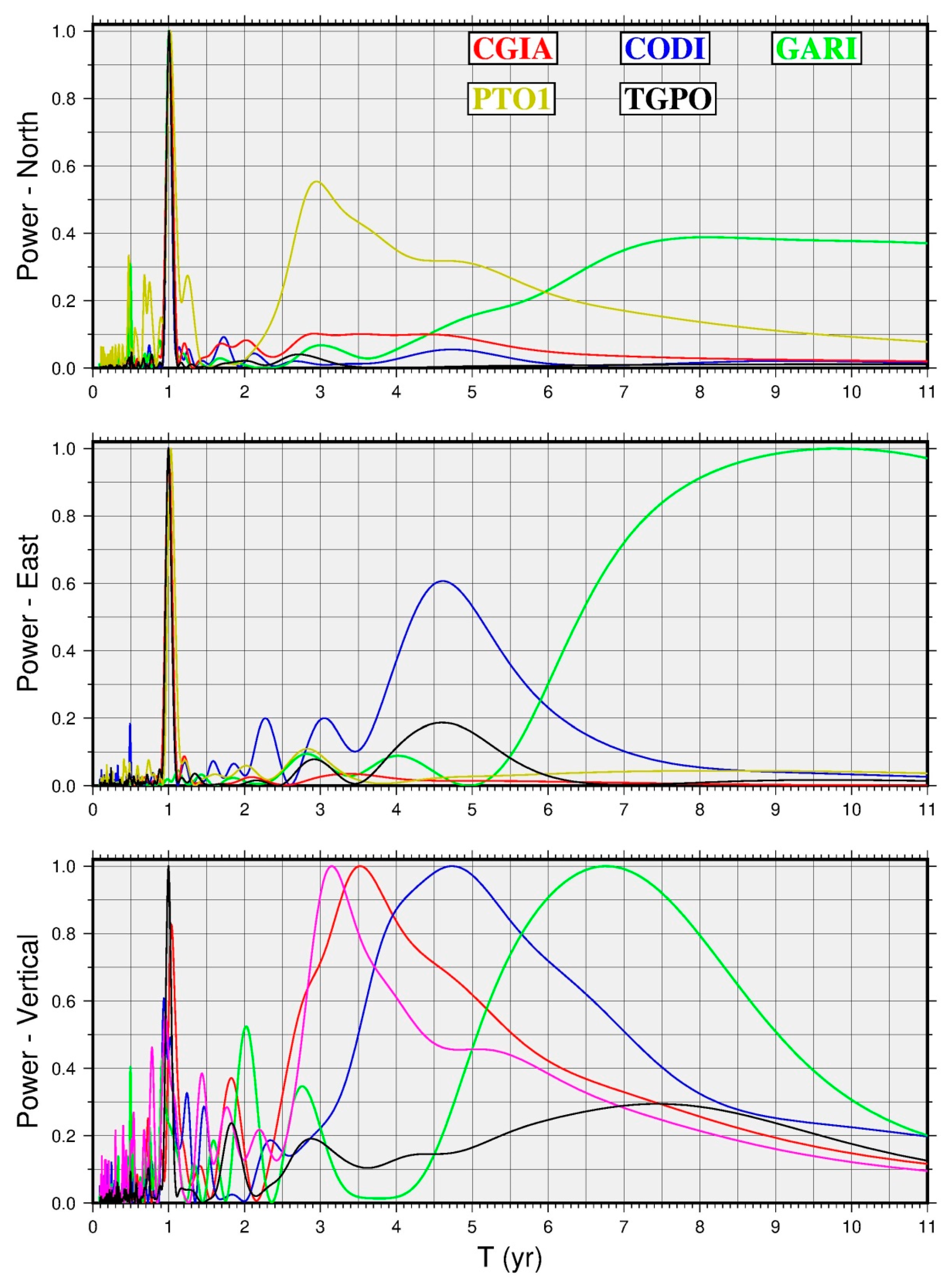
Figure 3.
IV time-series of the CGNSS sites located in the PRD area obtained using the Velocity Moving Window Approach (VMWA) with a window of 755 days (21 June 2016–18 July 2018). The windows containing less than 300 days were rejected. The black bars represent the uncertainties associated with the IV. The horizontal red lines represent the velocities obtained using the entire time-series and reported in Table 1. The purple vertical line represents the data related to the last day of the second PODELNET survey (18 July 2018). The IV associated with this data are the values corresponding to the time span between the two measurements.

Figure 4.
Vertical velocity field obtained analyzing the observations acquired during the two PODELNET surveys. Diamonds and squares show the position of the three CGNSS stations chosen as reference and benchmark sites, respectively. The background image is the geomorphological map shown in Figure 1 (a) and the Po Delta lobe generations map ((b), modified from Figure 13 in [72]); are also shown the positions of the seven Po River terminal branches.
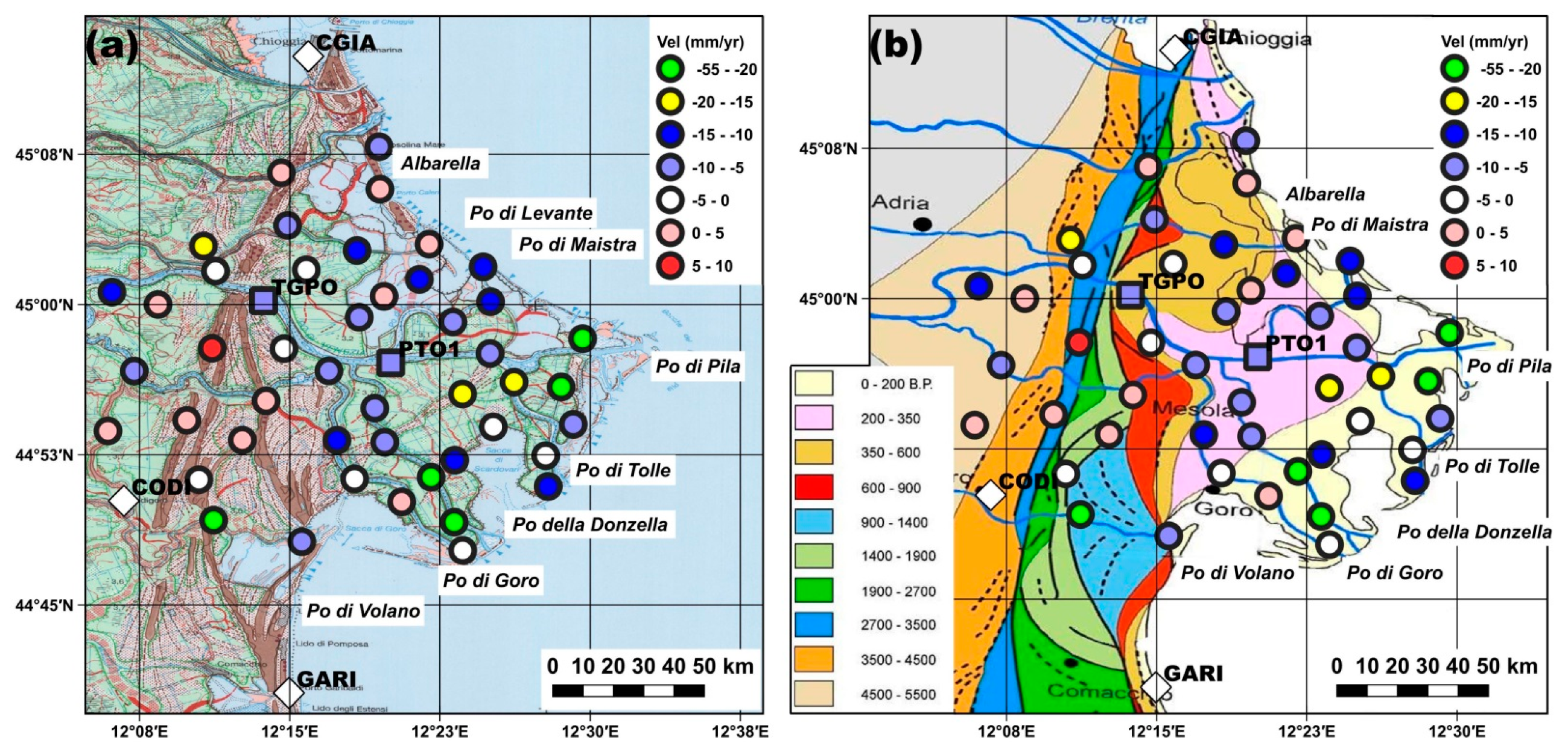
Figure 5.
IV time-series of the CGNSS sites located in the PRD area obtained using the VMWA with a window of 1128 days (the time span between the first and last InSAR images processed). The windows containing less than 500 days were rejected. We have analyzed the time series using the model described in equation 1 without discontinuities and significant seasonal signals and estimated by a weighted least square method. The black bars represent the uncertainties associated with the IV obtained with the weighted least square method used to compute the rates. The horizontal red lines represent the velocities obtained with the entire time series and are reported in Table 1. The purple vertical line represents the data related to the last day of the InSAR observations (17 May 2017). The IV associated with this data are the values corresponding to the time span between the InSAR images.

Figure 6.
Average InSAR velocity along the LOS direction at the CODI CGNSS site. (a) Average velocities with different search radiuses (from 20 m to 300 m, with a step of 10 m); the vertical bars are the calculated Weighted Root Mean Square (WRMS) values; (b) Number of InSAR points (Num. Point) used to obtain the average rate; (c) The mean distance (Mean Dist.) from the CGNSS site to the points included in the search area.
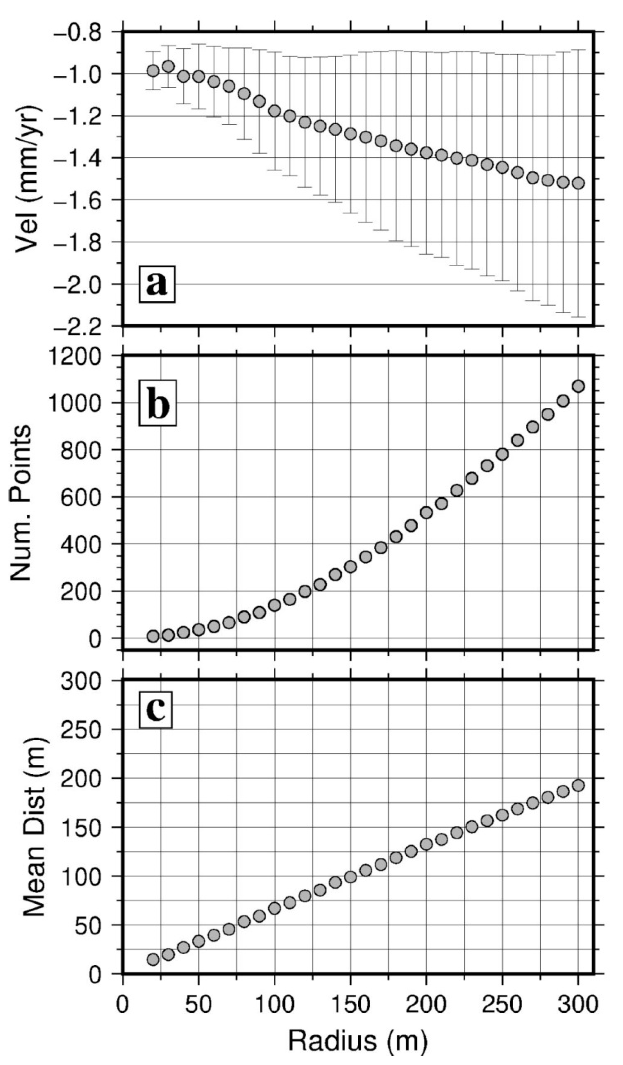
Figure 7.
Comparison between the InSAR and GNSS velocities; (a) The differences DV (VInSAR − VGNSS), in mm/year, between the interferometric and GNSS velocities; (b) The InSAR velocities were calculated averaging at least the rates of 6 points located at distances less than the radius. The figure shows the minimum radius needed to find at least 6 points in the searched area; (c) differences DV (VInSAR − VGNSS), in mm/year, between the rates compared to the radius used to obtain the InSAR velocities; (d) differences DV (VInSAR − VGNSS), in mm/year, compared to the number of points (Np) used to estimate the interferometric rates.

Figure 8.
(a) Velocity map along the LOS obtained analyzing the Sentinel-1A/B observations acquired from 2014 to 2017. The color of the circles represents the LOS PODELNET GNSS velocities (Table 3) overlapped to the InSAR kinematic pattern using the same scale; (b) Differences between InSAR and GNSS velocities (Table 3) at the PODELNET sites (VInSAR − VGNSS); are also shown the positions of the seven Po River terminal branches.


Table 1.
Velocities in mm/year of CGNSS stations located in the PRD and surrounding areas, adopted in the processing of the network as references (CGIA, CODI, GARI) and benchmarks (PTO1, TGPO). In the first and second columns are reported the CGNSS station codes and the date (T), in decimal year, of the first observation used in the processing, respectively. V are the velocities in the ETRF2014 reference frame [63] of the North (VN), East (VE), and Vertical (VV) components. The uncertainties associated with the velocities were estimated using the method suggested by [66]. The Weighted Root Means Square values (σ) in mm/year of the analyzed time-series are shown in the last three columns.
| Code | Start | T (year) | VN | VE | VV | σN | σE | σV |
|---|---|---|---|---|---|---|---|---|
| CGIA | 2011.3329 | 9.0 | 1.5 ± 0.6 | −0.2 ± 0.4 | −3.3 ± 0.6 | 1.1 | 1.4 | 3.2 |
| CODI | 2007.6315 | 12.1 | 1.6 ± 0.3 | −0.1 ± 0.4 | −3.5 ± 0.7 | 1.1 | 1.0 | 2.7 |
| GARI | 2009.5466 | 10.5 | 1.7 ± 0.3 | 0.1 ± 0.3 | −3.0 ± 0.5 | 1.1 | 0.9 | 3.7 |
| PTO1 | 2010.5575 | 9.3 | 1.7 ± 0.4 | −0.2 ± 0.3 | −5.8 ± 1.0 | 0.9 | 0.8 | 2.6 |
| TGPO | 2008.6544 | 11.3 | 1.5 ± 0.3 | −0.1 ± 0.3 | −5.6 ± 0.8 | 1.2 | 1.1 | 3.2 |
Table 2.
Velocities of the three components (North VN, East VE, and Vertical VV), in mm/year, of the continuous GNSS stations estimated by means of the Velocity Moving Window Approach (VMWA columns) using a window of 755 days (from 21 June 2016 to 18 July 2018). The values of the CGNSS sites estimated using only the observations acquired during the two campaigns are shown in the Campaigns columns, in mm/year; in the last three columns (Differences) are reported the differences between the corresponding values. The uncertainties associated with the VMWA velocities were obtained by a weighted least square approach adopted in the estimation of the velocities.
| VMWA | Campaigns | Differences | |||||||
|---|---|---|---|---|---|---|---|---|---|
| Code | VN | VE | VV | VN | VE | VV | VN | VE | VV |
| CGIA | 1.6 ± 0.5 | −1.0 ± 0.2 | −3.7 ± 0.4 | 2.1 | 0.3 | −3.1 | 0.5 | 1.4 | 0.6 |
| CODI | 1.6 ± 0.2 | 0.2 ± 0.2 | −3.1 ± 0.4 | 1.8 | −0.2 | −2.8 | 0.2 | −0.4 | 0.3 |
| GARI | 1.8 ± 0.2 | 0.0 ± 0.2 | −4.0 ± 0.6 | 1.1 | −0.9 | −4.9 | −0.7 | −1.0 | −0.9 |
| PTO1 | 1.5 ± 0.5 | −0.3 ± 0.3 | −5.8 ± 0.4 | 2.2 | 0.5 | −5.1 | 0.6 | 0.8 | 0.8 |
| TGPO | 1.8 ± 0.3 | 0.0 ± 0.2 | −6.5 ± 0.4 | 2.1 | −1.7 | −5.0 | 0.3 | −1.7 | 1.5 |
Table 3.
Velocities of the PODELNET sites were estimated by comparing the positions obtained analyzing the two surveys (2016–2018). The code of the PODELNET sites, defined by the IGMI, is reported in the first column; in the subsequent three columns are shown the geographical coordinates: Longitude and Latitude in centesimal degrees and the Height (H) in the WGS84 ellipsoid, in meters. The velocity components in mm/year along the North (VN), East (VE), and Vertical (VV) directions are also reported. The velocities along the LOS direction of Sentinel-1A/B satellites are shown in the VG column, in mm/year. The InSAR velocities, in mm/year, in the PODELNET sites are reported in VS column; DV are the differences, in mm/year, between the InSAR (VS) and GNSS (VG) velocities (DV = VS − VG). Np is the number of InSAR points used to obtain the VS rate, and R is the minimum radius, in meters, adopted to find the number of points. The values of PTO1 and TGPO permanent sites were obtained using only the observations acquired during the two PODELNET surveys and processed with the data of these campaigns.
| Code | Lon. | Lat. | H (m) | VN | VE | VV | VG | VS | DV | Np | R |
|---|---|---|---|---|---|---|---|---|---|---|---|
| 077703 | 12.260075 | 44.802738 | 43.642 | 5.1 | −0.1 | −8.0 | −6.8 | −6.1 | 0.7 | 7 | 30 |
| 065704 | 12.102026 | 45.010397 | 41.728 | 6.5 | −0.7 | −12.2 | −10.6 | −6.9 | 3.7 | 7 | 100 |
| 077704 | 12.186658 | 44.820580 | 41.325 | 5.4 | −1.4 | −27.5 | −32.8 | ||||
| 065705 | 12.263817 | 45.028918 | 43.585 | 5.6 | 0.8 | −3.5 | −2.7 | 0.1 | 2.8 | 6 | 180 |
| 065706 | 12.366029 | 45.050220 | 44.634 | −2.4 | −4.5 | 2.6 | −1.3 | −5.8 | −4.5 | 7 | 20 |
| 065707A | 12.178306 | 45.048738 | 43.832 | 3.0 | −16.5 | −15.8 | −25.1 | −1.9 | 23.2 | 7 | 40 |
| 077707 | 12.120610 | 44.944699 | 47.301 | 3.7 | −0.1 | −9.5 | −7.8 | −3.4 | 4.4 | 7 | 20 |
| 065708 | 12.243050 | 45.109684 | 46.692 | 3.2 | −1.7 | 1.6 | −0.4 | −4.5 | −4.2 | 10 | 50 |
| 077708 | 12.393936 | 44.795427 | 44.249 | 2.0 | 0.7 | −4.6 | −6.5 | ||||
| 077710 | 12.320833 | 44.913816 | 40.934 | 2.8 | −3.7 | −5.8 | −8.6 | ||||
| 077712 | 12.245224 | 44.963337 | 41.205 | 2.7 | 0.7 | −2.0 | −1.3 | −5.5 | −4.2 | 10 | 30 |
| 077713 | 12.416656 | 44.959307 | 45.740 | 3.9 | 0.0 | −6.6 | −10.5 | ||||
| 077714 | 12.282582 | 44.944837 | 41.129 | 4.8 | 3.4 | −5.0 | −1.8 | −5.9 | −4.1 | 7 | 30 |
| 065715 | 12.248242 | 45.065886 | 42.373 | −0.8 | −0.2 | −6.2 | −4.8 | −4.3 | 0.5 | 6 | 120 |
| 077715 | 12.329042 | 44.885502 | 42.578 | 0.1 | −3.3 | −7.3 | −8.2 | −5.9 | 2.3 | 7 | 210 |
| 077716 | 12.387378 | 44.870481 | 44.329 | 4.9 | 1.9 | −11.4 | −8.0 | −4.3 | 3.7 | 6 | 30 |
| 077717 | 12.386918 | 44.818930 | 39.585 | −1.4 | 1.4 | −52.7 | −40.3 | −8.6 | 31.7 | 7 | 150 |
| 077718 | 12.465061 | 44.848658 | 42.539 | 3.7 | −3.4 | −13.4 | −13.6 | −8.6 | 4.9 | 7 | 50 |
| 077719 | 12.419420 | 44.898224 | 45.138 | −0.3 | 1.6 | −1.6 | 0.1 | −8.6 | −8.6 | 9 | 50 |
| 077720 | 12.463006 | 44.874260 | 42.016 | 3.2 | 2.7 | −1.7 | 0.4 | −4.2 | −4.6 | 6 | 160 |
| 077721 | 12.367670 | 44.856351 | 40.282 | 3.2 | −2.7 | −23.2 | −20.6 | −6.2 | 14.4 | 6 | 80 |
| 077801 | 12.098680 | 44.894848 | 42.848 | −0.7 | 0.0 | 4.3 | 3.3 | −3.5 | −6.9 | 12 | 30 |
| 065901 | 12.328480 | 45.006855 | 52.369 | −1.5 | 0.7 | 0.1 | 0.8 | −5.0 | −5.8 | 9 | 50 |
| 077902 | 12.493799 | 44.971619 | 46.423 | 4.5 | 3.5 | −20.1 | −24.6 | 0.0 | 24.6 | 0 | 0 |
| 065903 | 12.324322 | 45.131373 | 44.721 | 3.3 | −0.8 | −8.8 | −7.8 | −3.9 | 3.9 | 10 | 30 |
| 077903 | 12.307800 | 44.989406 | 39.477 | 1.6 | 2.7 | −8.6 | −4.8 | −7.6 | −2.9 | 6 | 80 |
| 065904 | 12.325107 | 45.095947 | 43.359 | −1.2 | 0.5 | 0.1 | 0.6 | 0.6 | 0.0 | 6 | 220 |
| 077904 | 12.393814 | 44.925592 | 39.940 | 8.5 | 0.3 | −19.2 | −15.8 | −5.1 | 10.6 | 8 | 100 |
| 065905 | 12.188237 | 45.027850 | 53.072 | 5.3 | −2.0 | −5.0 | −5.9 | −2.8 | 3.1 | 7 | 80 |
| 077905 | 12.475986 | 44.931427 | 42.395 | 11.8 | −2.0 | −26.3 | −23.5 | −8.3 | 15.2 | 7 | 50 |
| 065906 | 12.410976 | 45.031372 | 46.199 | 5.5 | −0.3 | −13.6 | −19.1 | ||||
| 077906 | 12.485966 | 44.900349 | 44.585 | 2.5 | −1.0 | −6.8 | −6.4 | −7.9 | −1.5 | 7 | 60 |
| 065907 | 12.357916 | 45.020930 | 45.059 | 7.2 | 3.8 | −10.0 | −5.6 | −5.9 | −0.3 | 10 | 30 |
| 077907 | 12.210529 | 44.887197 | 40.944 | 7.7 | 3.6 | 0.4 | 2.3 | −4.4 | −6.7 | 12 | 30 |
| 065908 | 12.417091 | 45.002345 | 44.669 | 8.5 | 6.1 | −11.0 | −4.7 | −6.7 | −1.9 | 8 | 210 |
| 077908 | 12.303962 | 44.854954 | 43.110 | 0.3 | 1.0 | −4.9 | −3.1 | −5.2 | −2.1 | 13 | 30 |
| 065909 | 12.305983 | 45.044967 | 40.644 | 4.9 | −0.8 | −11.4 | −10.0 | −4.6 | 5.5 | 9 | 70 |
| 077909 | 12.385867 | 44.985537 | 39.513 | 7.4 | 2.2 | −7.8 | −5.2 | −8.4 | −3.2 | 6 | 190 |
| 077910 | 12.185478 | 44.963624 | 43.321 | −2.0 | −2.4 | 7.7 | 4.3 | −2.0 | −6.4 | 7 | 60 |
| 077911 | 12.436716 | 44.935469 | 50.726 | 2.0 | −0.2 | −18.0 | −14.5 | −6.2 | 8.3 | 8 | 30 |
| 077912 | 12.174395 | 44.854307 | 41.029 | −4.1 | −1.5 | −4.0 | −3.8 | −3.7 | 0.1 | 10 | 30 |
| 077913 | 12.164334 | 44.903659 | 40.262 | 3.5 | 3.0 | 1.1 | −2.3 | ||||
| 077914 | 12.230335 | 44.919938 | 41.848 | 6.8 | 2.8 | 2.8 | 3.6 | −3.9 | −7.5 | 7 | 20 |
| 077915 | 12.289302 | 44.887051 | 39.613 | 5.3 | 5.7 | −11.4 | −16.7 | ||||
| 077916 | 12.343223 | 44.835887 | 42.470 | 4.3 | 0.7 | 0.2 | 0.3 | −7.2 | −7.5 | 6 | 270 |
| 077917 | 12.140406 | 45.000043 | 42.242 | 1.3 | −0.4 | 1.5 | 0.7 | −2.9 | −3.7 | 6 | 230 |
| PTO1 | 12.334053 | 44.951520 | 49.311 | 2.2 | 0.5 | −5.1 | −3.8 | −4.3 | −0.5 | 11 | 30 |
| TGPO | 12.228321 | 45.003060 | 49.322 | 2.1 | −1.7 | −5.0 | −5.4 | −4.3 | 1.1 | 6 | 20 |
Table 4.
Velocities of the three components (North VN, East VE, and Vertical VV), in mm/year, of continuous GNSS stations obtained using the Velocity Moving Window Approach (VMWA columns) with a window of 1128 days. The velocities of the site CODI (Figure 1) were used in the reference translation procedure to align the InSAR velocities in the GNSS reference frame. VL, in mm/year, is the GNSS velocity along the LOS direction. VS, in mm/year, is the InSAR rate obtained averaging all the points in a 30 m radius. The differences between the InSAR rate and the LOS GNSS velocities of the benchmarks sites are also reported, in mm/year, in the VD column.
| VMWA | Number of Points | GNSS on LOS | InSAR LOS | Differences | |||
|---|---|---|---|---|---|---|---|
| Code | VN | VE | VV | VL | VS | VD | |
| CGIA | 1.5 ± 0.2 | −0.1 ± 0.2 | −3.6 ± 0.3 | - | - | - | - |
| CODI | 1.5 ± 0.2 | 0.0 ± 0.2 | −3.6 ± 0.3 | 8 | −2.9 | −2.9 | 0.0 |
| GARI | 1.4 ± 0.2 | 0.0 ± 0.2 | −3.9 ± 0.3 | - | - | - | - |
| PTO1 | 1.7 ± 0.2 | −0.1 ± 0.2 | −5.7 ± 0.3 | 11 | −4.8 | −4.3 | 0.5 |
| TGPO | 1.5 ± 0.2 | −0.1 ± 0.2 | −5.6 ± 0.3 | 8 | −4.6 | −4.3 | 0.3 |
Publisher’s Note: MDPI stays neutral with regard to jurisdictional claims in published maps and institutional affiliations. |
© 2021 by the authors. Licensee MDPI, Basel, Switzerland. This article is an open access article distributed under the terms and conditions of the Creative Commons Attribution (CC BY) license (https://creativecommons.org/licenses/by/4.0/).
Share and Cite
MDPI and ACS Style
Cenni, N.; Fiaschi, S.; Fabris, M. Monitoring of Land Subsidence in the Po River Delta (Northern Italy) Using Geodetic Networks. Remote Sens. 2021, 13, 1488. https://doi.org/10.3390/rs13081488
AMA Style
Cenni N, Fiaschi S, Fabris M. Monitoring of Land Subsidence in the Po River Delta (Northern Italy) Using Geodetic Networks. Remote Sensing. 2021; 13(8):1488. https://doi.org/10.3390/rs13081488
Chicago/Turabian StyleCenni, Nicola, Simone Fiaschi, and Massimo Fabris. 2021. "Monitoring of Land Subsidence in the Po River Delta (Northern Italy) Using Geodetic Networks" Remote Sensing 13, no. 8: 1488. https://doi.org/10.3390/rs13081488
Note that from the first issue of 2016, this journal uses article numbers instead of page numbers. See further details here.